Discovering Intrinsic Reward with Contrastive Random Walk

Given a Markov decision process (MDP), which can be described as $\mathcal{M}=\langle\mathcal{S},\mathcal{A},P,E,\gamma\rangle$, where $\mathcal{S}$ is the state space, $\mathcal{A}$ is the action space, $P\left(s_{t+1}\mid s_{t},a_{t}\right)$ is the probability distribution over transitions, $E\left(s_{t},a_{t}\right)$ is the environment reward function, and $\gamma$ is the discount factor. We will focus on infinite-horizon MDPs.

We define an exploration bonus based on the current state $I(s_{t})$ and add it to the reward $E\left(s_{t},a_{t}\right)$ given by the environment, getting a total reward $R\left(s_{t},a_{t}\right)=E\left(s_{t},a_{t}\right)+I(s_{t})$. The goal of the addition of exploration bonus is to embed the new reward to existing reinforcement learning algorithms and help to make a better policy.

The non-tabular environment of reinforcement learning can be viewed as an infinite-horizon stochastic dynamic programming, where states are some high-dimensional representations extracted by neural networks, denoted as $s=\phi(o)$, $s=[s_{1},s_{2},...,s_{n}]^{T}\in\mathbb{R}^{n}$, where $o$ is the observation (video frame). A prominent characteristic of non-tabular states is that the state representations are variant. As a neural network is applied and updated with experience, state representation of observations will change (i.e. $s$ will be updated with time). performance for count-based methods.

In order to make count-based methods also work for non-tabular state representations, discrete "counts" are changed into some density and continuous functions[3]. However, this approximation also incurs performance drop for count based methods. Therefore, curiosity methods are proposed to create a new kind of exploration bonus for non-tabular states.

Curiosity driven intrinsic rewards encourages the agent to explore the environment by learning an intrinsic reward $I(s_{t})$ besides the environment reward[5, 15, 4, 16, 6]. The intrinsic reward is given by neural network loss.

where C is a constant.

It applies the fact that if an input has been seen, loss of the neural network will decrease, indicating a lower intrinsic reward. Neural network loss style intrinsic reward also applies the generalization ability that makes it suitable for continuous state representation[13]. The loss will drop for exactly the same input $s_{t}$, but also states with similar feature to $s_{t}$, which makes it appropriate for non-tabular tasks.

There are mainly two types of curiosity methods: action dependent methods and state-only methods. State-only methods only use state representations from observations as inputs to the neural network[5, 16, 10]. Action dependent methods take both actions and state representations as input into neural networks[15, 6].

The information gain or mutual information is defined as:

It is widely used in Reinforcement learning as a measurement of intrinsic reward[3, 6].

For curiosity methods, information gain is made larger for unvisited states, while lower for frequently visited states to encourage the agent exploring the environment.

There exist various definitions of information gain in Reinforcement Learning[17, 20]. We will use the state-only transition information, which has been proved to be a good indicator for state representation[17].

In non-tabular scenario, we can change it to

. And the intrinsic reward for $s_{t+k}$ is thus

There are a bunch of previous works on how to extract better state representations[19, 12, 17, 7]. Better representations have been proved to be crucial to make RL algorithms perform better in many scenarios. Our work is most similar to [7], where the information gain is used to evaluate how good a representation is. The goal of this paper is to maximize information gain between inputs and outputs of the state encoder. Our method is also arguably increasing such information gain.

Since the environment we use is quite simple, the convergence of CRW is often too fast, and results in the intrinsic reward approaching zero with more iterations. Therefore, we applied the strategy of adaptive restart in optimization to settle the problem[14]. The parameters of CRW encoder are reset after the average intrinsic reward is smaller than a threshold. A psuedo code of our method can be found in Algorithm 1.

For the contrastive random walk,

where $\rho^{\prime}$ is the discounted state distribution for backtracing states, and $\rho$ is the discounted state distribution for forward states.

Because the backtracing gives exact the same states of forward path,

is not determined by the contrastive random walk, we just replace it by a constant $\mathrm{C}$.

Contrastive random walk optimizes the second term, such that:

Denote $P=\max p_{m}$, and when $P$ is close to 1, the above equation can be approximated by:

Remove the constant $M$, we get

This approximation is sufficient as the goal of contrastive random walk is to maximize $P$.

Thus, we can rewrite the information gain as:

Then, by optimizing the information gain of $s_{t+2k}$, we are also optimizing the information gain of $s_{t}$, as they share the same state representation.

To test the effectiveness of the exploration bonus we proposed, we combine our CRW Intrisic Reward with a Deep Q Network(DQN) backbone. Here we use a three-layer MLP with the default hidden dimensions (256,128,64) with 0.3 dropout ratio as our state encoder $\phi$ and Q-network. We compare our methods with several exploring baselines, which are Epsilon-greedy, Upper Confidence Bound (UCB), and Random Network Distillation(RND). These baseline models will use the same DQN as backbone. Q value is updated with the function

The target and predictor network of RND will share the same architecture of state encoder of our CRW. The main hyper-parameters and their default value used in the experiments are, temperature $\tau=1$, DQN learning rate $lr_{1}=1e-3$, state encoder learning rate $lr_{2}=1e-5$, restart running loss threshold $s=5e-3$, batch size $B=128$, replay buffer size $M=100000$, episode num $N=1000$. And the entire experiment is carried out on one NVIDIA RTX 3080 GPU. More details can be found in the code.

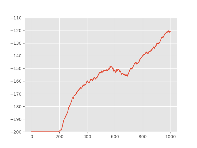
Here we report the performance of our CRW and other baselines in Figure 3. Our methods reach a final episode running reward of -110.607, which greatly surpasses all the other baselines, where epsilon greedy achieves -139.57, UCB achieves -121.037 and RND achieves -118.297. Meanwhile, we also observe that our methods begin to have rewards earlier than other networks. This phenomenon shows that our method wastes less efforts on testing a similar states, which benefits the convergence speed.

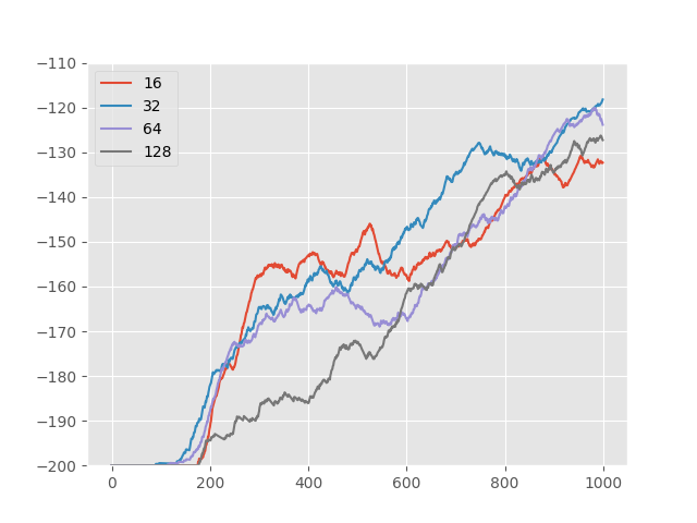
Here we show how each hyperparameter will contribute to the final results of our methods in Figure 4. The hyper-parameter tuned including feature dimension of the state encoder, temperature of crw, batch size during training and learning rate. Except for the parameter of being tuned, other parameters are set as default.

As shown in the results, temperature is an important factor to improve model performance. We find that the reward at 1000 iteration is linearly related to the choice of temperature. Generally, a small temperature with adaptive restart works better. Also, we found that adaptive restart is essential for CRW. When the restart threshold is set smaller, the performance of CRW may drop significantly.

For the agent network, we used an actor-critic architecture with cnn state encoder. We use a PPO [18] training method to update the networks, which is a same architecture suggested in the RND model [5]. To get the experience, we implement 64 workers using python multiprocessing. We also set the PPO learning rate $lr=1e-5$. For the CRW model that we proposed, we used a slightly different mean of encoding.

Because of the lack of computational resource, we just tried the implementation for 300 episodes and investigated the change of intrinsic reward. Because 300 episodes were not enough for the agent to get out of the first room, the implementation was in fact a purely exploration problem. As is shown in Figure 6, we can see that as the episode number increase, the intrinsic reward given by our CRW model first increase and then decrease, showing that the exploring first arise curiosity of the world, and then after many states are visited, the model lose the curiosity, thus the loss will drop to a lower value. This implies that our model can do the job of helping the algorithm to explore more unvisited states.

References

- [1] Peter Auer. Using confidence bounds for exploitation-exploration trade-offs. Journal of Machine Learning Research, 3(Nov):397–422, 2002.
- [2] M. G. Bellemare, Y. Naddaf, J. Veness, and M. Bowling. The arcade learning environment: An evaluation platform for general agents. Journal of Artificial Intelligence Research, 47:253–279, jun 2013.
- [3] Marc Bellemare, Sriram Srinivasan, Georg Ostrovski, Tom Schaul, David Saxton, and Remi Munos. Unifying count-based exploration and intrinsic motivation. Advances in neural information processing systems, 29, 2016.
- [4] Yuri Burda, Harri Edwards, Deepak Pathak, Amos Storkey, Trevor Darrell, and Alexei A Efros. Large-scale study of curiosity-driven learning. arXiv preprint arXiv:1808.04355, 2018.
- [5] Yuri Burda, Harrison Edwards, Amos Storkey, and Oleg Klimov. Exploration by random network distillation. arXiv preprint arXiv:1810.12894, 2018.
- [6] Ildefons Magrans de Abril and Ryota Kanai. Curiosity-driven reinforcement learning with homeostatic regulation. In 2018 international joint conference on neural networks (ijcnn), pages 1–6. IEEE, 2018.
- [7] R Devon Hjelm, Alex Fedorov, Samuel Lavoie-Marchildon, Karan Grewal, Phil Bachman, Adam Trischler, and Yoshua Bengio. Learning deep representations by mutual information estimation and maximization. arXiv preprint arXiv:1808.06670, 2018.
- [8] Allan Jabri, Andrew Owens, and Alexei Efros. Space-time correspondence as a contrastive random walk. Advances in neural information processing systems, 33:19545–19560, 2020.
- [9] Volodymyr Mnih, Koray Kavukcuoglu, David Silver, Andrei A Rusu, Joel Veness, Marc G Bellemare, Alex Graves, Martin Riedmiller, Andreas K Fidjeland, Georg Ostrovski, et al. Human-level control through deep reinforcement learning. nature, 518(7540):529–533, 2015.
- [10] Shakir Mohamed and Danilo Jimenez Rezende. Variational information maximisation for intrinsically motivated reinforcement learning. Advances in neural information processing systems, 28, 2015.
- [11] Andrew William Moore. Efficient memory-based learning for robot control. Technical report, University of Cambridge, 1990.
- [12] Ofir Nachum, Shixiang Gu, Honglak Lee, and Sergey Levine. Near-optimal representation learning for hierarchical reinforcement learning. arXiv preprint arXiv:1810.01257, 2018.
- [13] Behnam Neyshabur, Zhiyuan Li, Srinadh Bhojanapalli, Yann LeCun, and Nathan Srebro. Towards understanding the role of over-parametrization in generalization of neural networks. arXiv preprint arXiv:1805.12076, 2018.
- [14] Brendan O’donoghue and Emmanuel Candes. Adaptive restart for accelerated gradient schemes. Foundations of computational mathematics, 15(3):715–732, 2015.
- [15] Deepak Pathak, Pulkit Agrawal, Alexei A Efros, and Trevor Darrell. Curiosity-driven exploration by self-supervised prediction. In International conference on machine learning, pages 2778–2787. PMLR, 2017.
- [16] Deepak Pathak, Dhiraj Gandhi, and Abhinav Gupta. Self-supervised exploration via disagreement. In International conference on machine learning, pages 5062–5071. PMLR, 2019.
- [17] Kate Rakelly, Abhishek Gupta, Carlos Florensa, and Sergey Levine. Which mutual-information representation learning objectives are sufficient for control?, 2021.
- [18] John Schulman, Filip Wolski, Prafulla Dhariwal, Alec Radford, and Oleg Klimov. Proximal policy optimization algorithms, 2017.
- [19] Adam Stooke, Kimin Lee, Pieter Abbeel, and Michael Laskin. Decoupling representation learning from reinforcement learning. In International Conference on Machine Learning, pages 9870–9879. PMLR, 2021.
- [20] Stas Tiomkin and Naftali Tishby. A unified bellman equation for causal information and value in markov decision processes. arXiv preprint arXiv:1703.01585, 2017.