Discovering and Explaining the Non-Causality of Deep Learning in SAR ATR
Abstract
This is the pre-acceptance version, to read the final version please go to IEEE Geoscience and Remote Sensing Letters on IEEE Xplore. In recent years, deep learning has been widely used in SAR ATR and achieved excellent performance on the MSTAR dataset. However, due to constrained imaging conditions, MSTAR has data biases such as background correlation, i.e., background clutter properties have a spurious correlation with target classes. Deep learning can overfit clutter to reduce training errors. Therefore, the degree of overfitting for clutter reflects the non-causality of deep learning in SAR ATR. Existing methods only qualitatively analyze this phenomenon. In this paper, we quantify the contributions of different regions to target recognition based on the Shapley value. The Shapley value of clutter measures the degree of overfitting. Moreover, we explain how data bias and model bias contribute to non-causality. Concisely, data bias leads to comparable signal-to-clutter ratios and clutter textures in training and test sets. And various model structures have different degrees of overfitting for these biases. The experimental results of various models under standard operating conditions on the MSTAR dataset support our conclusions.
Index Terms:
Synthetic aperture radar (SAR), automatic target recognition (ATR), deep learning, data bias, Shapley value, causalityI Introduction
SYNTHETIC Aperture Radar (SAR) Automatic Target Recognition (ATR) is an essential branch of SAR image interpretation with significant promise for military and civilian applications[1, 2]. As deep learning has developed rapidly in this field, deep learning-based methods have achieved a recognition rate of over 99% percent for the benchmark dataset under Standard Operating Conditions (SOC)[1, 2].
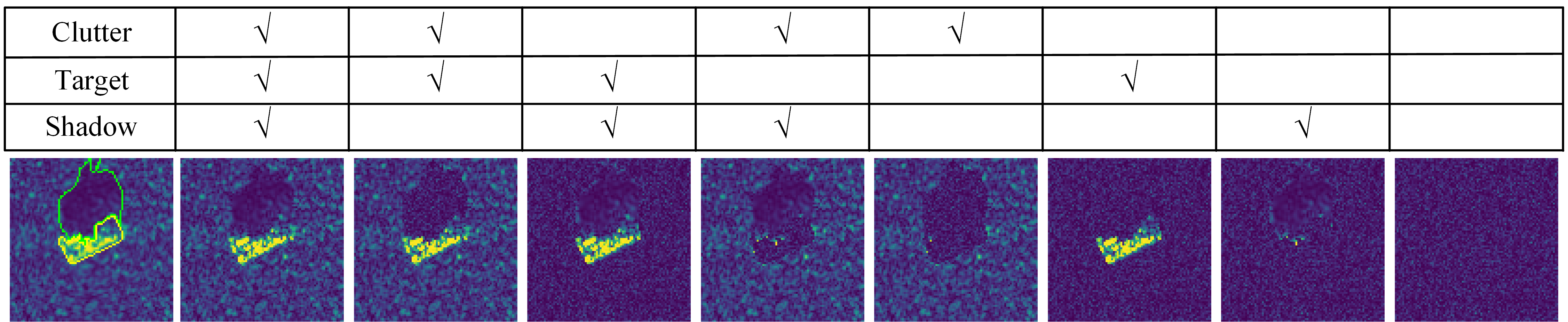
However, impressive performance does not mean deep learning correctly solves this recognition problem. The data and model affect the deep learning-based feature representation of SAR images. At the data level, the Moving and Stationary Target Acquisition and Recognition (MSTAR) benchmark dataset has data bias111Data bias refers to spurious correlations between target classes and non-causal features due to non-random collection conditions[3]. For example, the background contains no information about the target classes. Nevertheless, during data collection, the backgrounds of targets have differences across classes, which establishes a spurious correlation between backgrounds and target classes. (i.e., data selection bias). One of the obvious biases in MSTAR is background correlation[2]. This spurious correlation allows deep learning to exceed the recognition rate of random guesses when using background clutter slices without targets[2, 4, 5]. It is apparent from this phenomenon that clutter properties are class-related (i.e., clutter properties correlate with target classes) between the training set and the test set. However, to the best of our knowledge, researchers have yet to analyze the impact of background correlation on deep learning quantitatively. At the model level, deep learning can learn feature representation in a way that is unexpected to humans[6]. An example of model bias is texture222Texture refers to the spatial organization of a set of basic elements[7]. As shown in Fig. 1, the scattering point amplitude has different spatial distributions in the target, clutter, and shadow regions. These spatial distributions create texture signatures of different regions in SAR images. bias[8], i.e., deep learning relies on local texture rather than shape or contour for recognition. This problem is also present in SAR ATR due to imaging characteristics. SAR imaging reflects back-scattering intensity, which lacks the complete geometric structure and color of targets. As shown in Fig. 1, the main visual information is the scattering point distributions in the target and background regions, which reflect scattering point intensity and texture information. Therefore, deep learning can exploit the intensity and texture of background clutter.
Previous deep learning interpretability studies of SAR ATR [9, 10, 11] calculated the contribution of each single-pixel point in target, clutter, and shadow regions. Moreover, the ablation studies[11, 4, 5] described the influence of regions on the recognition rate. In particular, Belloni et al.[11] discussed the influence of different region permutations on the recognition rate of each class by ablation studies on target, clutter, and shadow regions. The above studies show that deep learning relies on target signatures and background clutter. The overfitting for background clutter reflects the incorrect feature representation and non-causality of deep learning. However, existing studies[11, 9, 10] focus on pixel-level contribution values and cannot quantitatively reflect the overall impact of different regions. It is also difficult to conclude intuitively from the recognition rates [11, 5] of target, clutter, and shadow permutations. Therefore, we improve how the saliency map divides images and calculates contributions. We analyze the contributions of different regions based on the Shapley value to provide quantitative indicators and clear conclusions.
This paper first analyzes the contributions and interactions of targets, clutter, and shadow regions during training. The contribution of clutter can be used as a quantitative indicator of the non-causality of deep learning. Next, we explain how data and model biases affect causality. The comparable signal-to-clutter ratios (SCR) and clutter texture establish a spurious correlation between target classes and background clutter. Deep learning can overfit these differences to reduce training errors. A re-weighting method is proposed to verify whether SCR is the cause of overfitting. Finally, we analyze the texture bias of the model structure with different parameters. The common phenomenon of various models in the MSTAR dataset supports our analysis and conclusions. The main contributions of this paper are as follows. Our code is available at https://github.com/waterdisappear/Data-Bias-in-MSTAR.
-
1.
We use the Shapley value and bivariate Shapley interactions to reflect the contribution and interactions of regions. These quantitative metrics can be used to analyze the feature representation of deep learning during training.
-
2.
Quantitative metrics allow us to analyze factors that impact deep learning causality. By intervening in the clutter SCR and model parameters, the quantitative metrics can clearly show the factors that influence overfitting for clutter.
II Methodology
II-A Shapley Value
Shapley value[12] is a method for calculating the player contribution solution in a cooperative game. This unique solution satisfies the four properties and is considered a fair attribution method[13, 14]. Consider is a set of all players with possible subsets. A game is a function that maps a subset to a real number. The Shapley value of -th player is given by:
| (1) |
where is a subset of , is the number of elements in the set. The Shapley value indicates whether -th player has a positive or negative impact on the outcome.
There are many variants for computing Shapley values in deep learning[15, 14], and we use the Baseline Shapley (BShap)[14]. The BShap is also the unique solution method that satisfies certain properties[14]:
| (2) |
where means that part of input retains its original value, while other parts are replaced with baseline . We set as the model classification score corresponding to the true class before Softmax333Since deep learning has saturated performance under SOC, we are more interested in the contribution of different regions to correct recognition during training. In addition, analyzing the causes of incorrect recognition in tests is also essential..
II-B Bivariate Shapley Interaction
The Bivariate Shapley Interaction (BSI)[13] is a way to measure the additional benefit of a coalition of two players and . The contribution of a coalition is often different from the sum of the individual players due to the influence of player interactions. For example, the shadow region responds to target shape information under specific sensor conditions and can form a coalition with the target region[11, 16]. The BSI can be defined below:
| (3) |
where , , , . The BSI describes whether an alliance between two players benefits the outcome.
II-C Random SCR Re-Weighting
The comparable SCR444Please refer to Fig. 3, which provides the comparable SCR curves across classes between the training and test sets is a brief representation of the background correlation. We propose a random SCR re-weighting method inspired by the re-weighting methods in causal inference[17]. We intend to create a similar SCR between classes to remove this spurious correlation. Our experiments show that this intervention reduces the overfitting for clutter, which shows that SCR is indeed one of the factors contributing to the background correlation. Alternatively, SCR re-weighting preserves the clutter texture, so we can further analyze the texture bias in various models.
First, the SCR of SAR images is defined as the ratio of the mean pixel value of target region to the mean pixel value of clutter region , i.e., . For the input magnitude image matrix , is sampled from a specific distribution555A uniform distribution is used to simulate random sampling, which keeps the SCR of different samples in the same 3 dB range. We aim to verify whether the comparable SCR leads to overfitting for clutter., such as a uniform distribution . We calculate the re-weighting factor and the re-weighting image is
| (4) |
where is the mask matrix of the clutter region, is a matrix whose elements are all one, is the Hadamard product.
III Experiments


III-A Data and Model
MSTAR, the most cited SAR ATR dataset in recent years, was collected by Sandia National Laboratory in the 1990s[1, 2]. The SAR images in JPEG format are generated by the official conversion tool666The official tool generates JPEG images by linear mapping and contrast enhancement. Since linear mapping normalizes the amplitude to [0, 255], we use SCR (a ratio) instead of amplitude to represent clutter properties. The contrast enhancement enhances the amplitude of targets and some clutter points. This method reduces A-ConvNet overfitting for clutter. and use SARbake777We use SARbake as a benchmark since it is an open-source dataset for segmentation. As SARbake uses 3D CAD models and projection relations to determine regions, some segmentation results do not completely match the actual SAR image. segmentation[18] as the ground truth for target, shadow, and clutter regions. SOC is the recognition of ten classes of targets[2]. The training and test sets are images of different azimuth angles in a similar scene888Although the scenes are all flat grasslands, factors such as the height, sparseness, and water content of vegetation can affect the scattering properties of background clutter., while the depression angle differs by 2°. The benchmark models are three deep learning models (A-ConvNet[19], AM-CNN[20], MVGGNet999MVGGNet used optical pre-training weights in the original paper. Considering our discussion of parameters, the optical pre-training weights are used for models with parameters larger than MVGGNet. Previous work[9] has shown that convolution kernels with pre-training have better texture and shape properties than direct training in the MSTAR dataset. We find this to be critical for ConvNeXtTiny. Optical pre-training weights reduced its overfitting for clutter and improved the test set accuracy from 55% to 98%.[21]) in SAR ATR and other models (EfficientNet[22], ResNet[23] and ConvNeXt[24]) in computer vision.
III-B Implementation Detail
The total score of BShap is . Therefore the baseline setting of Shapley values (i.e., absence of input variables) is essential. Belloni et al.[11] set the absence value to zero to calculate the recognition rate change. Considering the dark shadow region[11, 9], the absolute values of a Gaussian distribution are used in Fig. 1. This distribution differs from the target, clutter, and shadow areas to ensure that the total score reflects the differences. In the experiments, zero or noise baselines do not guarantee that is zero across classes. Moreover, various models have different classification scores . These cause the total score to vary across models, classes, and baselines. Therefore, we use the Shapley value ratio101010Due to the negative Shapley values, the Shapley value ratio is calculated by , where is the absolute value. to reflect the relative values. The Shapley values for the following experiments are the average of five replicate experiments, and Fig. 2 is the result of one.
III-C Discovering the Non-Causality
| Model | Region (SVR) | Coalition (BSI) | Accuracy | Params | |||||
|---|---|---|---|---|---|---|---|---|---|
| Clutter | Target | Shadow | Clutter&Target | Target&Shadow | Shadow&Clutter | Training | Test | ||
| A-ConvNet[19] | 35.91% (5.80) | 44.52% (7.19) | 19.57% (3.16) | 4.48 | 1.57 | 1.10 | 97.81% | 95.70% | 0.30M |
| AM-CNN[20] | 27.08% (2.71) | 53.23% (5.32) | 19.69% (1.97) | 3.86 | 2.87 | 1.20 | 100.0% | 97.17% | 2.60M |
| EfficientNet-B0[22] | 31.03% (4.49) | 40.79% (5.90) | 28.18% (4.08) | 3.05 | 1.75 | 1.93 | 99.40% | 92.83% | 4.02M |
| EfficientNet-B1[22] | 33.29% (4.63) | 38.16% (5.31) | 28.55% (3.97) | 3.29 | 1.95 | 1.50 | 99.51% | 93.06% | 6.53M |
| MVGGNet[21] | 34.21% (8.09) | 33.02% (7.81) | 32.77% (7.75) | 4.16 | 5.11 | 5.15 | 95.98% | 95.83% | 16.81M |
| ResNet34[23] | 39.39% (4.94) | 34.53% (4.33) | 26.08% (3.27) | 3.06 | 2.29 | 2.10 | 99.56% | 95.81% | 21.29M |
| ResNet50[23] | 37.80% (4.73) | 36.46% (4.57) | 25.74% (3.22) | 2.78 | 1.46 | 1.94 | 99.85% | 98.00% | 23.53M |
| ConvNeXtTiny[24] | 49.69% (5.38) | 27.35% (2.96) | 22.96% (2.49) | 2.11 | 0.40 | 1.34 | 99.84% | 98.19% | 27.83M |


Exp. 1, deep learning uses all correlations to reduce training errors, which does not guarantee causality. The recognition rate and Shapley values increase simultaneously during training in Fig. 2a. However, the Shapley value ratio shows different trends. The clutter curve undergoes an early rising process in Fig. 2b. This curve is because deep learning does not distinguish between correlations that come from causality and data bias. A-ConvNet initially focuses more on background differences. According to Table I, shadow areas have the least influence on recognition, with clutter and targets having the most influence. This finding is similar to the previous study[11]. In summary, the overfitting for clutter reflects the non-causality of deep learning.
Exp. 2, deep learning further exploits interactions between regions to reduce training errors. Fig. 2c shows that interactions between regions increase during training, indicating that the model can exploit correlations on a large scale. Both the target and shadow regions contain class information, but the model also uses clutter differences to form a coalition. Table I shows that the strength of coalition interaction varies across models. Hence, the interactions of regions in deep learning are also influenced by biases.
III-D Explaining the Non-Causality
Exp. 3, data bias leads to class-related clutter properties, one of which is the comparable SCR curves between the training and test sets. According to the SCR curves in Fig. 3, the background clutter is comparable for different target classes in MSTAR. Due to background correlation in training and test sets, overfitting for clutter does not significantly reduce performance under SOC in Table I. Interestingly, the target region contributes negatively to the results when A-ConvNet recognizes the four lowest SCR classes in Fig 3. This phenomenon indicates that the model learns incorrect feature representations to recognize some classes. Similarly, removing targets does not affect the recognition rate for some classes in [11]. Another similar case in computer vision is using snowy backgrounds to distinguish between wolves and huskies[25]. Despite the impressive performance in Table I, our work illustrates that background correlation results in deep learning-based feature representations that are incorrect but valid for biased datasets.

Exp. 4, deep learning models can use background clutter texture for recognition. Fig. 4 shows that clutter contribution is reduced by eliminating the comparable SCR. This result also confirms that comparable SCR is one of the factors contributing to background correlation. As our method only changes the amplitude of clutter, the texture remains intact111111The relative intensity of clutter scattering points still maintains the original spatial distribution, which keeps a local repeating clutter texture in SAR images.. Our experimental results suggest that the model can more memorize clutter texture in datasets when its capacity increases significantly with the parameter121212We use parameters to measure different models. In fact, many factors influence texture bias. We find that optimization methods and model structures affect clutter contribution. Therefore, we use the same optimizer. Furthermore, special model structures such as batch normalization and attentional mechanisms need to be discussed to investigate whether the texture bias is discrepant for the target or clutter..
IV Conclusion
We analyzed the non-causality of deep learning in SAR ATR based on the Shapley value. Data and model biases lead to non-causality and overfitting for background clutter in deep learning. Background correlation leads to comparable SCR and clutter texture in MSTAR, and the models with different parameters have different degrees of overfitting to these clutter properties. In addition, overfitting for clutter is normally hidden by the background correlation of the MSTAR dataset and the black-box property of deep learning. Our analysis indicates that the causality and robustness of deep learning in SAR ATR are still under consideration. Since clutter is color noise, overfitting for clutter implies non-robustness in various environments. Moreover, causal features (i.e., target signatures) are unstable under different imaging conditions. Current adversarial attack studies have shown that deep learning is affected by small shifts in target signatures[26, 27]. A small dataset such as MSTAR can not adequately reflect target and background variations across imaging conditions, even with reduced data bias. It remains to be explored whether deep learning can achieve robust SAR ATR. Deep learning requires causality to suppress clutter and be robust to shifts in target signatures for real-world applications.
References
- [1] E. Blasch, U. Majumder, E. Zelnio, and V. Velten, “Review of recent advances in AI/ML using the MSTAR data,” Proc. 27th SPIE Conf. Algorithms SAR Imagery, vol. 11393, pp. 53–63, 2020.
- [2] O. Kechagias-Stamatis and N. Aouf, “Automatic target recognition on synthetic aperture radar imagery: A survey,” IEEE Aerosp. Electron. Syst. Mag., vol. 36, no. 3, pp. 56–81, 2021.
- [3] P. Cui and S. Athey, “Stable learning establishes some common ground between causal inference and machine learning,” Nat. Mach. Intell., vol. 4, no. 2, pp. 110–115, 2022.
- [4] F. Zhou, L. Wang, X. Bai, and Y. Hui, “SAR ATR of ground vehicles based on LM-BN-CNN,” IEEE Trans. Geosci. Remote Sens., vol. 56, no. 12, pp. 7282–7293, 2018.
- [5] R. Schumacher and J. Schiller, “Non-cooperative target identification of battlefield targets-classification results based on SAR images,” in Proc. IEEE Int. Radar Conf, 2005, pp. 167–172.
- [6] Q. Zhang, W. Wang, and S. Zhu, “Examining CNN representations with respect to dataset bias,” in Proc. AAAI Conf. Artif. Intell. (AAAI), vol. 32, no. 1, 2018.
- [7] L. Liu, J. Chen, P. Fieguth, G. Zhao, R. Chellappa, and M. Pietikäinen, “From BoW to CNN: Two decades of texture representation for texture classification,” Int. J. Comput. Vision, vol. 127, pp. 74–109, 2019.
- [8] B. Shi, D. Zhang, Q. Dai, Z. Zhu, Y. Mu, and J. Wang, “Informative dropout for robust representation learning: A shape-bias perspective,” in Int. Conf. Machin. Learn. (ICML), 2020, pp. 8828–8839.
- [9] W. Li, W. Yang, Y. Liu, and X. Li, “Research and exploration on the interpretability of deep learning model in radar image (in chinese),” Sci. Sin. Inform., vol. 52, p. 1114–1134, 2022.
- [10] M. Heiligers and A. Huizing, “On the importance of visual explanation and segmentation for SAR ATR using deep learning,” in Proc. IEEE Radar Conf. (RadarConf), 2018, pp. 0394–0399.
- [11] C. Belloni, A. Balleri, N. Aouf, J.-M. Le Caillec, and T. Merlet, “Explainability of deep SAR ATR through feature analysis,” IEEE Trans. Aerosp. Electron. Syst., vol. 57, no. 1, pp. 659–673, 2020.
- [12] L. S. Shapley, “A value for n-person games,” in Contributions to the Theory of Games, vol. 2, 1953, p. 307–317.
- [13] H. Zhang, Y. Xie, L. Zheng, D. Zhang, and Q. Zhang, “Interpreting multivariate shapley interactions in dnns,” in Proc. AAAI Conf. Artif. Intell. (AAAI), vol. 35, no. 12, 2021, pp. 10 877–10 886.
- [14] M. Sundararajan and A. Najmi, “The many Shapley values for model explanation,” in Int. Conf. Machin. Learn. (ICML), 2020, pp. 9269–9278.
- [15] S. M. Lundberg and S.-I. Lee, “A unified approach to interpreting model predictions,” Proc. Adv. Neural Inf. Process. Syst. (NeurIPS), vol. 30, 2017.
- [16] J.-H. Choi, M.-J. Lee, N.-H. Jeong, G. Lee, and K.-T. Kim, “Fusion of target and shadow regions for improved SAR ATR,” IEEE Trans. Geosci. Remote Sens., vol. 60, pp. 1–17, 2022.
- [17] L. Yao, Z. Chu, S. Li, Y. Li, J. Gao, and A. Zhang, “A survey on causal inference,” ACM Trans. Knowl. Discovery Data, vol. 15, no. 5, pp. 1–46, 2021.
- [18] D. Malmgren-Hansen, M. Nobel-J et al., “Convolutional neural networks for SAR image segmentation,” in Proc. IEEE Int. Symp. Signal Process. Inf. Technol., 2015, pp. 231–236.
- [19] S. Chen, H. Wang, F. Xu, and Y. Jin, “Target classification using the deep convolutional networks for SAR images,” IEEE Trans. Geosci. Remote Sens., vol. 54, no. 8, pp. 4806–4817, 2016.
- [20] M. Zhang, J. An, L. D. Yang, L. Wu, X. Q. Lu et al., “Convolutional neural network with attention mechanism for SAR automatic target recognition,” IEEE Geosci. Remote Sens. Lett., vol. 19, pp. 1–5, 2020.
- [21] J. Zhang, M. Xing, and Y. Xie, “FEC: A feature fusion framework for SAR target recognition based on electromagnetic scattering features and deep cnn features,” IEEE Trans. Geosci. Remote Sens., vol. 59, no. 3, pp. 2174–2187, 2020.
- [22] M. Tan and Q. Le, “Efficientnet: Rethinking model scaling for convolutional neural networks,” in Int. Conf. Machin. Learn. (ICML), 2019, pp. 6105–6114.
- [23] K. He, X. Zhang, S. Ren, and J. Sun, “Deep residual learning for image recognition,” in Proc. IEEE Comput. Soc. Conf. Comput. Vis. Pattern Recognit. (CVPR), 2016, pp. 770–778.
- [24] Z. Liu, H. Mao, C.-Y. Wu, C. Feichtenhofer, T. Darrell, and S. Xie, “A convnet for the 2020s,” in Proc. IEEE Comput. Soc. Conf. Comput. Vis. Pattern Recognit. (CVPR), 2022, pp. 11 976–11 986.
- [25] R. Fjelland, “Why general artificial intelligence will not be realized,” Humanit. Social Sci. Commun., vol. 7, no. 1, pp. 1–9, 2020.
- [26] B. Peng, B. Peng, J. Zhou, J. Xia, and L. Liu, “Speckle-variant attack: Toward transferable adversarial attack to SAR target recognition,” IEEE Geosci. Remote Sens. Lett., vol. 19, pp. 1–5, 2022.
- [27] B. Peng, B. Peng, J. Zhou, J. Xie, and L. Liu, “Scattering model guided adversarial examples for SAR target recognition: Attack and defense,” IEEE Trans. Geosci. Remote Sens., vol. 60, pp. 1–17, 2022.