Discover governing differential equations from evolving systems
Abstract
Discovering the governing equations of evolving systems from available observations is essential and challenging. In this paper, we consider a new scenario: discovering governing equations from streaming data. Current methods struggle to discover governing differential equations with considering measurements as a whole, leading to failure to handle this task. We propose an online modeling method capable of handling samples one by one sequentially by modeling streaming data instead of processing the entire dataset. The proposed method performs well in discovering ordinary differential equations (ODEs) and partial differential equations (PDEs) from streaming data. Evolving systems are changing over time, which invariably changes with system status. Thus, finding the exact change points is critical. The measurement generated from a changed system is distributed dissimilarly to before; hence, the difference can be identified by the proposed method. Our proposal is competitive in identifying the change points and discovering governing differential equations in three hybrid systems and two switching linear systems.
I Introduction
Research on the hidden information in measurements that performs a transformative impact on the discovery of dynamical systems has attracted the attention of scientific researchers [1, 2, 3, 4]. Many canonical dynamics are rooted in conservation laws and phenomenological behaviors in physical engineering and biological science [5]. Enabled by the increasing maturity of sensor technology, data-driven methods have promoted various innovations in describing time series generated from experiments [4]. Due to the complexity of dynamical systems, revealing the underlying governing equations representing the physical laws from time-series data that gives a general description of the spatiotemporal activities is a tremendous challenge [3, 6, 7, 8, 9, 10, 11, 12].
In a series of developments, modeling methods for complex systems include empirical dynamic modeling [13], equation-free modeling [14, 15], and modeling emergent behavior [16]. Discovery patterns contain normal form identification [17], nonlinear Laplacian spectral analysis [18], dynamic automatic inference [19], and nonlinear regression [20]. Overall, popular methods for data-driven discovery of complex systems are mainly based on sparse identification [21, 22] and deep neural networks [23, 24], such as sparse identification of nonlinear dynamics (SINDy) [25] and PDE-Net [26]. Existing methods have provided an encouraging performance on systems motivated by unchanging rules or architectures, where novelty and variability are seen as disruptive [27].
However, although capable of effectively handling spatiotemporal sequences, the above algorithms are batch learning methodologies whose common problem is ephemeral fitting [13, 28], thereby leading to the abortive modeling for streaming data consecutively generated like water flow. The overwhelming majority of complex systems are constantly running and generating new observations one by one over time (such as financial markets, social networks, and neurological connectivity, etc.) [29, 30, 31, 32], resulting in failing to update gradients in the SINDy. In real-time systems, we must adapt to different stream parts and produce an immediate output before seeing the next input.
Moreover, several SINDy-based methods have been demonstrated to perform online tasks. Autoencoder SINDy is trained offline and queried online to compute the time evolution of the full order system in different conditions [33]. [34] claims that the SINDy-based algorithm holds feasibility in online applications due to its few computational time for all cases, owing to a little tuning of parameters and Fast Fourier Transform. However, these methods cannot handle streaming data and discover the change points in evolving systems. The most related work is the method in [35], which processes solution snapshots that arrive sequentially. It is a small batch method. Its performance and training iterations depend on the length of snapshots, which will seriously affect the evaluation of change points. Thus, [35] has difficulty finding the change point hidden in solution snapshots on account of the nature of the mini-batch method, which limits the application of this method to switching systems.
To the concrete, we regard the measurements reflecting the system status as invariably changing streaming data. In this article, we present a novel method, called Online-Sparse Identification of Nonlinear Dynamics (O-SINDy), to develop a parsimonious model that most accurately represents the real-time streaming data. Our proposal handles samples sequentially by modeling subsampled spatiotemporal sequences as streaming measurements instead of processing the entire dataset directly. Moreover, O-SINDy can bypass batch storage and intractable cases of combinatorial brute-force search across all possible candidate terms.
Mathematically, we conduct experiments with diverse spatiotemporal measurements generated from dynamical systems to verify the excellent performance of O-SINDy. By recovering extensively representative physical system expressions solely from streaming data, the method is demonstrated to work on various canonical instances, including the nonlinear Lorenz system, Burgers’ equation, reaction-diffusion equation, etc. Experimental results show that our framework provides an online technique for real-time online analysis of complex systems. We suggest that O-SINDy, which overcomes the limitations of batch learning methodologies, is competent for deducing the governing differential equations if sequential measurements of complex dynamic systems are available.
With the ability to handle streaming data, O-SINDy can ideally cope with the parameter estimation of time-varying nonlinear dynamics and is general enough to detect multiple types of evolutionary patterns. O-SINDy outperforms the state-of-the-art methods in discovering governing differential equations in the evolving two-dimensional damped harmonic oscillators, Susceptible-Infected-Recovered disease model with time-varying transmission rates, and two switching linear systems.
II Methods
With large amounts of data arriving as streams, any offline machine learning algorithm that attempts to store the complete dataset for analysis will fail due to running out of memory. The rise of streaming data raises the technical challenge of a real-time system, which must do any processing or learning encouraged by each record in arriving order. Let denote the state vector of a real-time system at time , and represent its partial differentiation in time domain. The system receives streaming inputs:
For instance, vector represents the position information of the particle shown in Fig. 1(a). Every step, the particle moves along the trajectory; the data will be captured by sensors and sent to the system that needs to analyze or respond in time. Instead of storing the entire stream, continuous online learning faces one input at a time.
The rigorous model of a complex system is always a set of differential equations with unknown physics parameters [36]. Without losing generality, we consider a general parameterized physical system of the following form:
| (1) |
where the terms with subscript represent partial differentiation of in space domain, “1” denotes the constant, and is an unknown combination of the nonlinear functions, partial derivatives, constant, and additional terms of . Our goal is to select the correct terms that are most relevant to dynamic information on real-time circumstance. In view of measurements of all considered state variables , the right-hand side of Eq. (1) can be expressed by multiplying the library function matrix with the coefficient matrix as follows:
| (2) |
where
| (3) |
Columns of , , correspond to specific candidate terms for the governing equation, as shown in Fig. 1(b).
O-SINDy is divided into two steps: (i) build complete libraries of candidate terms; (ii) update the structure of governing equations via the FTRL-Proximal style methodology. Each procedure is described as follows.
II.1 Build a candidate library
We start by collecting the spatiotemporal series data at time points and spatial locations of the state variables. For each state variable, the captured state measurements are represented as a single column state vector . Based on all the observables, e.g., variables , , and in Lorenz systems, a series of functional terms associated with these quantities can be calculated and then reshaped into a single column as well, such as , , , , etc. Likewise, partial differential terms should be considered in the candidate library if PDEs govern the dynamics. Furthermore, “1” denotes the constant term that possibly appears in equations. The compositive function library is a matrix that contains designed functional terms. Note that the computed time derivative is also a single-column vector presented on the left-hand side of Eq. (2). The constant term in the library sufficiently considers the bias term in the governing differential equation so that the model can be regarded as an unbiased representation of dynamics. For O-SINDy, an important prerequisite for revealing the correct governing differential equation is that the candidate function library contains all the members which constitute the concise dynamics expression, so as to ensure that the exact sparse coefficient is computed under iterations.
II.2 Optimization
Formulating a hypothesis that the governing differential equations are evolving at any moment, we model each example as a dynamic process to simulate the arrival of streaming data. Given a set of time-series state measurements at a fixed number of spatial locations in , the goal is to construct the form of online. To fix this issue, the core of our innovation is utilizing real-time streaming data to denote the loss function. Considering a coefficient vector in , , which corresponds to the specific state variable , the fitness function is designed as follows:
| (4) |
where denotes the regularization coefficient, is the number of positions, denotes the length of the time series, , and is defined as follows:
| (5) |
where is the time derivative of the th state observation, is the th row of the common library that represents all candidate function values for the ith data. The sparsity constraints mean that the coefficient vector is sparse with only a few non-zero entries, each representing a subsistent item in the function library. Subsequently, we exploit the follow-the-regularized-leader (FTRL)-Proximal [37, 38, 39] style methodology to optimize the outcome by considering solely one instance each time.
Leveraging the fact that each instance is considered individually, we rewrite the loss function and define a single loss term (see Eq. (5)). For example, if the first state measurement is available, the loss is defined as: . Next, if the second instance of arrives, the loss is defined as: . In this way, the computer only needs to store information about a single example, thus relieving memory stress. On the th sample, the gradient is calculated as follows:
| (6) |
Normally, the online gradient descent algorithm can be used to update the coefficient vector after the arrival of the th data by using:
| (7) |
However, this method has been proven to lack general applicability [38]. Correspondingly, the FTRL-proximal style approach is introduced to solve the online problem. We use the following equation to update the coefficient vector :
| (8) | |||||
where and both denote the regularization coefficient, which is the positive constant, while is on the th learning rate aspect, defined by:
| (9) |
Given the gradient a shorthand , we set . Then the update in Eq. (8) can be rewritten as follows:
where the last term is a constant with respect to and negligibly impacts the update process. Let , and we ignore the last term and rewrite Eq. (II.2) as:
| (11) |
Let and represent the th element of the vector and , respectively. Equation (9) is generalized as
| (12) | |||||
Aiming to simplify the expression, we suppose to be the optimal solution of and to be its gradient. Then, Eq. (13) is satisfied. Equation (17) shows the subdifferential of .
| (13) |
| (17) |
The solution to can be discussed in three cases [40]:
- 1.
- 2.
- 3.
The above discussion in different estimation scenarios is summarized in Eq. (22), where .
| (22) |
Moreover, we set a remarkable learning rate
| (23) |
where and are both positive constants, denotes the th element of the gradient and is the learning rate of . Thus, Eq. (9) can be rewritten as follows:
| (24) |
The final form of the closed solution is obtained and expressed as
| (27) |
where and are both positive constants, denotes the th element of the gradient .
Notably, is always updated according to the current input instance, thereby guiding the detection of change points if there exists any variation in the evolving system. Additionally, the mechanism frees the computer from storing the whole large-scale data. It should be highlighted that the method suggested above is entirely different from the batch learning methods, which update gradients depending on all available measurements. O-SINDy 111Available code: https://github.com/xiaoyuans/O-SINDy. takes advantage of a single available instance and updates gradients based on the current loss in each iteration, thereby being easily extended to handle evolving systems. Note that the optimum selection of hyper-parameters in each case is determined by grid search ().
| Dynamic System | Identified Governing Equation | Error | Setting |
| Harmonic oscillator1 | 1.62e-05 | , | |
| Harmonic oscillator2 | 6.28e-04 | , | |
| Lorenz system 1 | 2.80e-04 | ||
| Lorenz system 2 | 2.70e-04 | ||
| Hopf normal form | 1.85e-02 | , | |
| Diffusion from random walk | 1.69e-05 | , | |
| Burgers’ | 6.97e-04 | ||
| Korteweg-de Vries (KdV) | 2.17e-02 | , | |
| Kuramoto-Sivashinsky | 2.55e-02 | , | |
| Reaction-diffusion | 2.65e-04 | , , | |
III Results
III.1 Discovering Single System from Streaming Data
III.1.1 Example – Discovering Chaotic Lorenz System
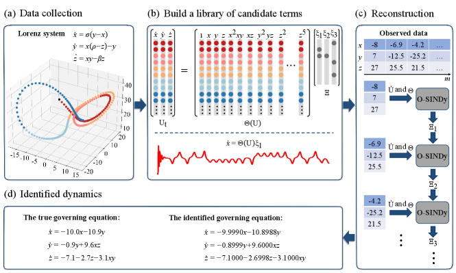
The online algorithmic procedure for identifying correct governing differential equations of the chaotic Lorenz system from time series is demonstrated in Fig. 1. Our proposal combines data collection, a library of potential candidate functions, and the online reconstruction method. The Lorenz system is highly nonlinear described by the following equations, according to which we construct a canonical dynamic instance for model discovery.
| (28) | |||
| (29) | |||
| (30) |
To indicate the nonlinear combination of Lorenz variables, common parameters are , =8/3, and =28, with the initial condition of . Ref. [3] has employed the SINDy autoencoder to discover a parsimonious model with only seven active terms that seems to mismatch the original Lorenz system. Interestingly, the dynamics of the resulting model exhibit an attractor with a 2-lobe structure, which is qualitatively consistent with the true Lorentz attractor. Then the sparsity pattern can be rewritten in the standard form by choosing an appropriate variable transformation. Considering the chaotic nature, O-SINDy show the ability to capture the concise model on two Lorenz systems. Results in Fig. 1(d) and Table 1 imply that O-SINDy can accurately reproduce the attractor dynamics from chaotic trajectory measurements. In both cases, we conducted 10000 timesteps with time intervals =0.01.
Given time intervals and initial conditions, we simulate the Lorenz system within a certain time horizon. Specifically, state measurements are collected under the constraints of the transformed expressions, including historical data of the state and its time derivative . The combination of spatial and temporal modes results in the trajectory of dynamics shown in Fig. 1(a). A library of potential candidate functions, , is constructed to find the least terms required to satisfy . Candidate functions can be polynomial functions, trigonometric functions, exponential functions, logarithmic functions, partial derivatives, constant items, and any additional terms about . The proposed online technique can identify the coefficient to determine active terms of the dynamics. To elude the obstacle of large-scale data storage and batch gradient update, we design a cumulative loss function to reflect the mode of streaming data by solely analyzing the information of one sample at a time. The pre-established sparse scenario guarantees that the resulting solution obtained by the online method can effectively balance model complexity with description ability to avoid overfitting, thereby promoting its interpretability and extensibility. The prompt update of components and coefficients in the governing equation is one implementation of data arrival based synchronization. Consequently, we can subtly detect moderate or drastic variations in the system through changes in the resulting model.
III.1.2 Performance on Discovery for Canonical Models
We perform O-SINDy on ten canonical models in mathematical physics and engineering sciences, and the results are shown in Table 1. These physical systems contain dynamics with periodic to chaotic behavior, ranging from linear to strongly nonlinear systems. The settings for spatial and temporal sampling and the coefficient errors are detailed in Table 1. Encouragingly, O-SINDy can recover every physical system, even those with significant spatial subsampling. The notable results highlight the broad applicability of the method and the success of this online technique in discovering governing differential equations. Remarkably, the capacity for capturing nontrivial active terms, in particular, has essential explanatory implications for model discovery.
| Methodology | Cubic_Linear | KdV_KS |
|---|---|---|
| O-SINDy | Phase 1 | Phase 1 |
| Phase 2 | Phase 2 | |
| STRidge [4] | ||
| TrainSTRidge [4] | ||
| STLS [42] | ||
| Lasso [21] | ||
| ElasticNet [43] | ||
| FoBaGreedy [44] | ||
III.2 Discovering Hybrid Systems
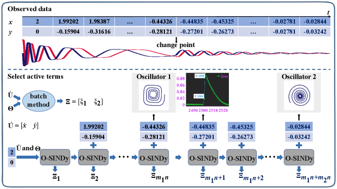
We first consider an evolving two-dimensional damped harmonic oscillator that changes from cubic to linear.
| (31) |
| (32) |
A particle in simple harmonic vibration is known as a harmonic oscillator, whose motion is the simplest ideal vibration model. Fig. 2 illustrates the dynamic data and the detection of change points. Firstly, we create the solution to Eq. (32), , with 2,500 timesteps and the initial data . Then, we utilize the last instance in as the initial data and create the solution to Eq. (31) with 2,500 timesteps as well, recorded as . Specifically, the change point arises when the system changes, and then the original distribution of generated data varies. Therefore, the corresponding loss value gradually decreases and stabilizes unless the change point appears. In this context, the coefficients in the former governing equation and the change location are simultaneously identified according to the sudden increase of loss value.
With an augmented nonlinear library including polynomials up to the fifth order, the change point is spotted in evolving circumstances. The loss curve tends to stabilize faster after resetting the training coefficient, thereby accelerating the convergence of O-SINDy because the former result may mislead the training process.
The transition from the KdV to the Kuramoto-Sivashinsky equation is simulated as an illustrative example that exhibits qualitatively different dynamics as the system evolves. Summary of O-SINDy and the state-of-the-art methods in SINDy for this identification in Table 2 demonstrates that our approach works well. Most data-driven methods regard batch measurements as a whole and update gradients integrally to obtain an ephemeral fitting. Owing to the ignorance of variations, existing methodologies are biased to strike a compromise solution, so that strenuous to identify the changes from consecutively generated data. Quite the contrary, O-SINDy succeeds in simultaneously estimating forms and identifying changes of the governing equations.
Moreover, we investigate the Susceptible-Infected-Recovered (SIR) disease model with time-varying transmission rates, widely studied in epidemiology [45, 46]. The following equation is a mathematical description of the SIR model.
| (33) | |||
| (34) | |||
| (35) | |||
| (38) |
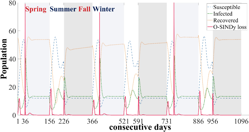
It is a time-dependent hybrid dynamical system, where , is the total population, , , and is a base transmission rate. We simulate the model for three years within the initial condition at , recording at a daily interval. A random perturbation is added to the start of each season with the same probability.
To illustrate the dynamics of the SIR model, we display the recovered population by subtracting 920 and scaling the loss in O-SINDy by the maximum value. As shown in Fig. 3, O-SINDy captures the transition between states by the dramatically increasing loss. In this example, the perturbation is able to be identified utilizing solely the information of the recovered population, which is ignored in Hybrid-Sparse Identification of Nonlinear Dynamics (Hybrid-SINDy)[46]. It is an offline batch learning method and outputs the governing equation of a single day by repeatedly clustering the whole time-series data during the model selection step. The identified governing equations of four random days in the four seasons are summarized in Table 3. The results show that O-SINDy provides more precise reconstruction accuracy for a single day. Specifically, instances of the same coefficients share the hyper-parameters in O-SINDy. At the same time, Hybrid-SINDy selects a model of the highest frequency from results recovered by SINDy with different hyper-parameters for each certain instance. Moreover, the effect of cluster size is particularly vital to solutions in Hybrid-SINDy.
| Datetime | True models | O-SINDy | Hybrid-SINDy |
|---|---|---|---|
| 30 | |||
| 80 | |||
| 184 | |||
| 350 | |||
III.3 Discovering Switching Linear Systems
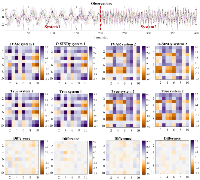
We also test O-SINDy on two switching linear systems, including synthetic and real-world datasets. Define as the sampled trajectory of a dynamical system, is the feature dimension. Time-varying autoregressive model with low-rank tensors (TVART) [47] holds the assumption, , where is constant within a time window but varies in the switching system. On the contrary, O-SINDy discards the time window and admits that may change at every time point.
Regarding the synthetic example, we randomly generate two system matrices and to encourage the switching system. The dynamics follow and switch to after half of the time series. Results illustrated in Fig. 4 show that O-SINDy is competitive with the state-of-the-art technique TVART.
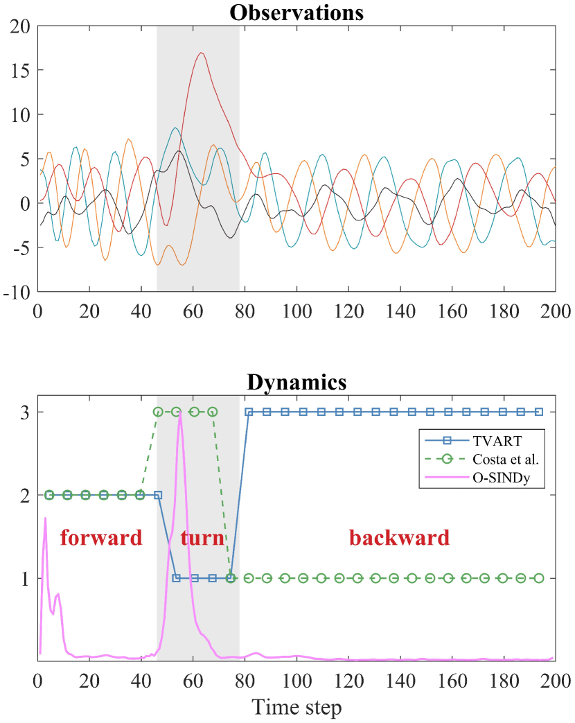
The posture dynamics of the worm Caenorhabditis elegans [48, 49] is studied as the real-world example for clustering via adaptive, locally linear models [50]. This time-series data details the escape behavior of the worm in response to a heat stimulus, e.g., the transition from forward, turn, to backward crawling. Fig. 5 characterizes the true dynamics and the discovered modes corresponding to its three typical dynamical regimes. It should be highlighted that the bifurcation of the worm dynamics is interpretable on a smaller time scale with the application of O-SINDy.
IV Conclusion and Discussion
We have proposed an online modeling method, O-SINDy, capable of finding governing differential equations of evolving systems from streaming data. We demonstrate that O-SINDy works on various canonical instances. Results in Table 1 indicate that the inference of governing equation is accurate when utilizing O-SINDy on time series from numerical simulations. Additionally, we show the excellent performance of simultaneously estimating forms and identifying changes in time-varying dynamic systems.
More sampling points or longer time series correspond to the preferable identification of the internal control structure, while the KdV equation is an exception (see Table 4). One potential viewpoint is that approximating the soliton solution introduces great uncertainty. Nevertheless, it remains an open question to estimate the required time-series length for distilling the accurate underlying governing differential equations. The implementation of existing methodologies fundamentally depends on sufficiently large datasets, even though the dynamics are only a parsimonious representation. O-SINDy, on the contrary, is demonstrated to recover the true governing equations by iteratively reusing the finite available time series. Note that the computation of time derivatives results in the main error, which is magnified by the numerical roundoff. Thus, correctly estimating numerical derivatives is the most critical and challenging task for O-SINDy, especially in a noisy context.
O-SINDy is a viable tool capable of tackling streaming data from evolving systems for accomplishing the assignment of model discovery. The integration opens up a novel, interesting research insight for real-time modeling, online analysis, and control techniques of complex dynamic systems.
| Discretization | =3 | =6 | =10 | =10 | =6 |
| =256 | =256 | =256 | =128 | =128 | |
| Error | 0.2807 | 0.0217 | 0.0090 | 0.0972 | 0.0068 |
Acknowledgements.
This work was supported in part by the National Natural Science Foundation of China under Grant 62206205, in part by the Fundamental Research Funds for the Central Universities under Grant XJS211905, in part by the Guangdong High-level Innovation Research Institution Project under Grant 2021B0909050008, and in part by the Guangzhou Key Research and Development Program under Grant 202206030003.Appendix A Data Preprocessing
For massive-scale datasets, sparse sampling can be used to reduce the data size. For identification, it should be noted that we only require a small number of spatial points and their neighbors, whose responsibility is estimating the partial derivative terms in the candidate library. That is, local information around each measurement is necessarily wanted. Distinction allowing for application to subsampled spatiotemporal sequences, to an extent, is critically important due to experimentally and computationally prohibitive implementation of collecting full-state measurements [4]. In terms of derivation, second-order finite differences [51] are devoted to the clean data from numerical simulations, while the easiest to implement and most reliable method for the noisy data is a polynomial interpolation [52]. In principle, we abandon those points close to the boundaries due to the absence of numerical derivatives. If we know any prior knowledge about the governing equation, for instance, if one of the potential terms is determined to be nonzero in advance, we can apply the additional information to the initialization phase. Moreover, truncation of the solution is a tool to maintain its sparsity, and different threshold values may provide distinguishing sparsity levels of the final output. As for the artificial noise added to the state measurements of governing equations, we use white noise. The noisy data is directly trained in experiments. In terms of the reaction-diffusion equation, exceptionally, we use the singular value decomposition (SVD) [53] to denoise some noisy spatiotemporal series, and the result is a low-dimensional approximation of datasets.
Appendix B Canonical Models
B.1 Reaction Diffusion
The dynamic of reaction-diffusion systems is defined by the following equations, which provide great expressiveness and freedom although they are deceptively simple.
| (39) | |||
| (40) |
where , , and . Given the vast number of data points, we subsample 5000 discretized spatial points with 30 time points each.
B.2 Hopf Norm Form
In this example, the application of O-SINDy is extended to a parameterized normal form of Poincaré-Andronov-Hopf bifurcation.
| (41) | |||
| (42) |
We explored a normal form of Hopf bifurcation on two-dimensional ordinary differential equations systems. Given and , we collected data from the noise-free system for eight various values of the parameter .
B.3 Fokker-Planck Equation
Fokker-Planck equation that reflects the connection between the diffusion equation and Brownian motion has been taken into account. Considering the simplest form of the diffusion equation where the diffusion coefficient is 0.5 and the drift term is zero, the corresponding Fokker-Planck equation is . The Brownian motion model is usually simplified as a random walk in physics, such as the random movement of molecules in liquids and gases. To simulate the process, we add a distributed random variable with variance to the time series and sample the movement of the random walker.
B.4 Burgers’ Equation
Here, we consider a fundamental partial differential equation in the fields of fluid mechanics, nonlinear acoustics, and aerodynamics. As a dissipative system in one-dimensional space, the general form of Burgers’ equation is described by a diffusion coefficient (also known as kinematic viscosity). The speed of the fluid at the indicated spatial coordinate and temporal coordinate in a thin ideal pipe can be expressed as the following equation:
| (43) |
where the diffusion term contributes the advective form of the Burgers’ equation.
B.5 Korteweg-de Vries Equation
The Korteweg-de Vries (KdV) equation is a nonlinear, partial differential equation for a function of two real variables, and , which refer to space and time, respectively. Numerically, its solutions seem to be decomposed into a collection of well-separated solitary waves that are almost unaffected in shape by passing through each other. The soliton solution is given by
| (44) |
where stands for the phase speed, is an arbitrary constant and is the hyperbolic secant function. This equation describes a right-moving soliton that propagates with a speed proportional to the amplitude.
The correct equation cannot be distinguished from a single propagating soliton solution, due to the fact that some studied expressions may be solutions to more than one PDE [4]. For example, both the one-way wave equation and the KdV equation admit the same traveling wave solution of the form if the initial data was a hyperbolic secant squared. Hence, we constructed time-series data for more than a single initial amplitude to rectify the ambiguity in selecting the governing PDE, thereby enabling the unique determination.
As the circumstance under a single propagating soliton solution, we respectively constructed two solutions without noise having the traveling speed equal to 5 or 1 on grids with 6 timesteps and 256 spatial points. Ultimately, corresponding advection equations with different were identified using a single traveling wave. We believe that two waves with different amplitudes and speeds may solve the KdV equation.
B.6 Kuramoto-Sivashinsky Equation
The Kuramoto-Sivashinsky (KS) equation is a fourth-order nonlinear PDE derived by Yoshiki Kuramoto and Gregory Sivashinsky in the late 1970s. Specifically, it provides two dissipative terms and based on Burgers’ equation, where the fourth-order diffusion term accomplishes the stabilizing regularization rather than the second-order diffusion term , which leads to long-wavelength instabilities. By leveraging a spectral method, the numerical solution to the KS equation was created with 101 timesteps and 1024 spatial points.
References
- Sugihara and May [1990] G. Sugihara and R. M. May, Nonlinear forecasting as a way of distinguishing chaos from measurement error in time series, Nature 344, 734 (1990).
- Tropp and Gilbert [2007] J. A. Tropp and A. C. Gilbert, Signal recovery from random measurements via orthogonal matching pursuit, IEEE Transactions on Information Theory 53, 4655 (2007).
- Champion et al. [2019] K. Champion, B. Lusch, J. N. Kutz, and S. L. Brunton, Data-driven discovery of coordinates and governing equations, Proceedings of the National Academy of Sciences 116, 22445 (2019).
- Rudy et al. [2017] S. H. Rudy, S. L. Brunton, J. L. Proctor, and J. N. Kutz, Data-driven discovery of partial differential equations, Science advances 3, e1602614 (2017).
- Crutchfield and McNamara [1987] J. P. Crutchfield and B. McNamara, Equations of motion from a data series, Complex Systems 1, 417 (1987).
- Li et al. [2019] S. Li, E. Kaiser, S. Laima, H. Li, S. L. Brunton, and J. N. Kutz, Discovering time-varying aerodynamics of a prototype bridge by sparse identification of nonlinear dynamical systems, Physical Review E 100, 022220 (2019).
- Reinbold and Grigoriev [2019] P. A. K. Reinbold and R. O. Grigoriev, Data-driven discovery of partial differential equation models with latent variables, Physical Review E 100, 022219 (2019).
- Maddu et al. [2021] S. Maddu, B. L. Cheeseman, C. L. Müller, and I. F. Sbalzarini, Learning physically consistent differential equation models from data using group sparsity, Physical Review E 103, 042310 (2021).
- Somacal et al. [2022] A. Somacal, Y. Barrera, L. Boechi, M. Jonckheere, V. Lefieux, D. Picard, and E. Smucler, Uncovering differential equations from data with hidden variables, Physical Review E 105, 054209 (2022).
- Shea et al. [2021] D. E. Shea, S. L. Brunton, and J. N. Kutz, Sindy-bvp: Sparse identification of nonlinear dynamics for boundary value problems, Physical Review Research 3, 023255 (2021).
- Xu and Zhang [2021] H. Xu and D. Zhang, Robust discovery of partial differential equations in complex situations, Physical Review Research 3, 033270 (2021).
- Chen et al. [2022] Y. Chen, Y. Luo, Q. Liu, H. Xu, and D. Zhang, Symbolic genetic algorithm for discovering open-form partial differential equations (sga-pde), Physical Review Research 4, 023174 (2022).
- Ye et al. [2015] H. Ye, R. J. Beamish, S. M. Glaser, S. C. Grant, C.-h. Hsieh, L. J. Richards, J. T. Schnute, and G. Sugihara, Equation-free mechanistic ecosystem forecasting using empirical dynamic modeling, Proceedings of the National Academy of Sciences 112, E1569 (2015).
- Kevrekidis et al. [2003] I. G. Kevrekidis, C. W. Gear, J. M. Hyman, P. G. Kevrekidis, O. Runborg, C. Theodoropoulos, et al., Equation-free, coarse-grained multiscale computation: enabling microscopic simulators to perform system-level analysis, Commun. Math. Sci 1, 715 (2003).
- Proctor et al. [2014] J. L. Proctor, S. L. Brunton, B. W. Brunton, and J. Kutz, Exploiting sparsity and equation-free architectures in complex systems, The European Physical Journal Special Topics 223, 2665 (2014).
- Roberts [2014] A. J. Roberts, Model emergent dynamics in complex systems, Vol. 20 (SIAM, 2014).
- Majda et al. [2009] A. J. Majda, C. Franzke, and D. Crommelin, Normal forms for reduced stochastic climate models, Proceedings of the National Academy of Sciences 106, 3649 (2009).
- Giannakis and Majda [2012] D. Giannakis and A. J. Majda, Nonlinear laplacian spectral analysis for time series with intermittency and low-frequency variability, Proceedings of the National Academy of Sciences 109, 2222 (2012).
- Daniels and Nemenman [2015] B. C. Daniels and I. Nemenman, Automated adaptive inference of phenomenological dynamical models, Nature Communications 6, 1 (2015).
- Voss et al. [1999] H. U. Voss, P. Kolodner, M. Abel, and J. Kurths, Amplitude equations from spatiotemporal binary-fluid convection data, Physical Review Letters 83, 3422 (1999).
- Tibshirani [1996] R. Tibshirani, Regression shrinkage and selection via the lasso, Journal of the Royal Statistical Society. Series B (Methodological) 58, 267 (1996).
- Mangan et al. [2016] N. M. Mangan, S. L. Brunton, J. L. Proctor, and J. N. Kutz, Inferring biological networks by sparse identification of nonlinear dynamics, IEEE Transactions on Molecular, Biological and Multi-Scale Communications 2, 52 (2016).
- Brunton and Kutz [2022] S. L. Brunton and J. N. Kutz, Data-driven science and engineering: Machine learning, dynamical systems, and control (Cambridge University Press, 2022).
- Lusch et al. [2018] B. Lusch, J. N. Kutz, and S. L. Brunton, Deep learning for universal linear embeddings of nonlinear dynamics, Nature communications 9, 1 (2018).
- Brunton et al. [2016] S. L. Brunton, J. L. Proctor, and J. N. Kutz, Discovering governing equations from data by sparse identification of nonlinear dynamical systems, Proceedings of the National Academy of Sciences 113, 3932 (2016).
- Long et al. [2018] Z. Long, Y. Lu, X. Ma, and B. Dong, Pde-net: Learning pdes from data, in International Conference on Machine Learning (PMLR, 2018) pp. 3208–3216.
- Hallac et al. [2017] D. Hallac, Y. Park, S. Boyd, and J. Leskovec, Network inference via the time-varying graphical lasso, in Proceedings of the 23rd ACM SIGKDD International Conference on Knowledge Discovery and Data Mining (2017) pp. 205–213.
- Ranjan [2014] R. Ranjan, Modeling and simulation in performance optimization of big data processing frameworks, IEEE Cloud Computing 1, 14 (2014).
- Namaki et al. [2011] A. Namaki, A. H. Shirazi, R. Raei, and G. Jafari, Network analysis of a financial market based on genuine correlation and threshold method, Physica A: Statistical Mechanics and its Applications 390, 3835 (2011).
- Ahmed and Xing [2009] A. Ahmed and E. P. Xing, Recovering time-varying networks of dependencies in social and biological studies, Proceedings of the National Academy of Sciences 106, 11878 (2009).
- Myers and Leskovec [2010] S. Myers and J. Leskovec, On the convexity of latent social network inference, Advances in Neural Information Processing systems 23 (2010).
- Monti et al. [2014] R. P. Monti, P. Hellyer, D. Sharp, R. Leech, C. Anagnostopoulos, and G. Montana, Estimating time-varying brain connectivity networks from functional mri time series, NeuroImage 103, 427 (2014).
- Cai et al. [2022] Y. Cai, X. Wang, G. Joos, and I. Kamwa, An online data-driven method to locate forced oscillation sources from power plants based on sparse identification of nonlinear dynamics (sindy), IEEE Transactions on Power Systems (2022).
- Conti et al. [2023] P. Conti, G. Gobat, S. Fresca, A. Manzoni, and A. Frangi, Reduced order modeling of parametrized systems through autoencoders and sindy approach: continuation of periodic solutions, Computer Methods in Applied Mechanics and Engineering 411, 116072 (2023).
- Messenger et al. [2022] D. A. Messenger, E. Dall’Anese, and D. Bortz, Online weak-form sparse identification of partial differential equations, in Mathematical and Scientific Machine Learning (PMLR, 2022) pp. 241–256.
- Schaeffer et al. [2013] H. Schaeffer, R. Caflisch, C. D. Hauck, and S. Osher, Sparse dynamics for partial differential equations, Proceedings of the National Academy of Sciences 110, 6634 (2013).
- McMahan [2011] B. McMahan, Follow-the-regularized-leader and mirror descent: Equivalence theorems and l1 regularization, in Proceedings of the Fourteenth International Conference on Artificial Intelligence and Statistics (2011) pp. 525–533.
- McMahan et al. [2013] H. B. McMahan, G. Holt, D. Sculley, M. Young, D. Ebner, J. Grady, L. Nie, T. Phillips, E. Davydov, D. Golovin, et al., Ad click prediction: a view from the trenches, in Proceedings of the 19th ACM SIGKDD International Conference on Knowledge Discovery and Data Mining (2013) pp. 1222–1230.
- Wu et al. [2022] K. Wu, X. Hao, J. Liu, P. Liu, and F. Shen, Online reconstruction of complex networks from streaming data, IEEE Transactions on Cybernetics 52, 5136 (2022).
- Chen et al. [2001] S. S. Chen, D. L. Donoho, and M. A. Saunders, Atomic decomposition by basis pursuit, SIAM Review 43, 129 (2001).
- Note [1] Available code: https://github.com/xiaoyuans/O-SINDy.
- Budišić et al. [2012] M. Budišić, R. Mohr, and I. Mezić, Applied koopmanism, Chaos: An Interdisciplinary Journal of Nonlinear Science 22, 047510 (2012).
- Zou and Hastie [2005] H. Zou and T. Hastie, Regularization and variable selection via the elastic net, Journal of the royal statistical society: series B (statistical methodology) 67, 301 (2005).
- Zhang [2008] T. Zhang, Adaptive forward-backward greedy algorithm for sparse learning with linear models, Advances in neural information processing systems 21, 1921–1928 (2008).
- Grenfell et al. [1994] B. T. Grenfell, A. Kleckzkowski, S. Ellner, and B. Bolker, Measles as a case study in nonlinear forecasting and chaos, Philosophical Transactions of the Royal Society of London. Series A: Physical and Engineering Sciences 348, 515 (1994).
- Mangan et al. [2019] N. M. Mangan, T. Askham, S. L. Brunton, J. N. Kutz, and J. L. Proctor, Model selection for hybrid dynamical systems via sparse regression, Proceedings of the Royal Society A 475, 20180534 (2019).
- Harris et al. [2021] K. D. Harris, A. Aravkin, R. Rao, and B. W. Brunton, Time-varying autoregression with low-rank tensors, SIAM Journal on Applied Dynamical Systems 20, 2335 (2021).
- Stephens et al. [2008] G. J. Stephens, B. Johnson-Kerner, W. Bialek, and W. S. Ryu, Dimensionality and dynamics in the behavior of c. elegans, PLoS computational biology 4, e1000028 (2008).
- Broekmans et al. [2016] O. D. Broekmans, J. B. Rodgers, W. S. Ryu, and G. J. Stephens, Resolving coiled shapes reveals new reorientation behaviors in c. elegans, Elife 5, e17227 (2016).
- Costa et al. [2019] A. C. Costa, T. Ahamed, and G. J. Stephens, Adaptive, locally linear models of complex dynamics, Proceedings of the National Academy of Sciences 116, 1501 (2019).
- LeVeque [2007] R. J. LeVeque, Finite difference methods for ordinary and partial differential equations: steady-state and time-dependent problems (SIAM, 2007).
- Bruno and Hoch [2012] O. Bruno and D. Hoch, Numerical differentiation of approximated functions with limited order-of-accuracy deterioration, SIAM Journal on Numerical Analysis 50, 1581 (2012).
- Gavish and Donoho [2014] M. Gavish and D. L. Donoho, The optimal hard threshold for singular values is , IEEE Transactions on Information Theory 60, 5040 (2014).
- Walters [1987] C. J. Walters, Nonstationarity of production relationships in exploited populations, Canadian Journal of Fisheries and Aquatic Sciences 44, s156 (1987).
- Sugihara et al. [2012] G. Sugihara, R. May, H. Ye, C.-h. Hsieh, E. Deyle, M. Fogarty, and S. Munch, Detecting causality in complex ecosystems, Science 338, 496 (2012).
- Zhu and Xu [2005] X. Zhu and J. Xu, Estimation of time varying parameters in nonlinear systems by using dynamic optimization, in 31st Annual Conference of IEEE Industrial Electronics Society, 2005. IECON 2005. (2005) pp. 5 pp.–.
- Kolar et al. [2010] M. Kolar, L. Song, A. Ahmed, and E. P. Xing, Estimating time-varying networks, The Annals of Applied Statistics , 94 (2010).
- Deyle et al. [2013] E. R. Deyle, M. Fogarty, C.-h. Hsieh, L. Kaufman, A. D. MacCall, S. B. Munch, C. T. Perretti, H. Ye, and G. Sugihara, Predicting climate effects on pacific sardine, Proceedings of the National Academy of Sciences 110, 6430 (2013).
- Candès et al. [2006] E. J. Candès, J. Romberg, and T. Tao, Robust uncertainty principles: Exact signal reconstruction from highly incomplete frequency information, IEEE Transactions on Information Theory 52, 489 (2006).
- Ruelle and Takens [1971] D. Ruelle and F. Takens, On the nature of turbulence, Communications in Mathematical Physics 20, 167 (1971).
- Bramburger et al. [2020] J. J. Bramburger, D. Dylewsky, and J. N. Kutz, Sparse identification of slow timescale dynamics, Physical Review E 102, 022204 (2020).
- Dylewsky et al. [2022] D. Dylewsky, E. Kaiser, S. L. Brunton, and J. N. Kutz, Principal component trajectories for modeling spectrally continuous dynamics as forced linear systems, Physical Review E 105, 015312 (2022).
- Tran et al. [2023] M.-Q. Tran, T. T. Tran, P. H. Nguyen, and G. Pemen, Sparse identification for model predictive control to support long-term voltage stability, IET Generation, Transmission & Distribution 17, 39 (2023).