Direct measurement of non-thermal electron acceleration from magnetically driven reconnection in a laboratory plasma
Abstract
Magnetic reconnection is a ubiquitous astrophysical process that rapidly converts magnetic energy into some combination of plasma flow energy, thermal energy, and non-thermal energetic particles, including energetic electrons Yamada, Kulsrud, and Ji (2010); Ji et al. (2022). Various reconnection acceleration mechanisms Blandford et al. (2017); Guo et al. (2020) in different low- (plasma-to-magnetic pressure ratio) and collisionless environments Masuda et al. (1994); Øieroset et al. (2002); Krucker et al. (2010); Abdo et al. (2011); Tavani et al. (2011); Chen et al. (2020) have been proposed theoretically and studied numerically Drenkhahn and Spruit (2002); Sironi and Spitkovsky (2014); Werner et al. (2016); Li et al. (2017); Guo et al. (2020); Dahlin (2020), including first- and second-order Fermi acceleration Drake et al. (2006), betatron acceleration Hoshino et al. (2001), parallel electric field acceleration along magnetic fields Egedal, Le, and Daughton (2013), and direct acceleration by the reconnection electric field Zenitani and Hoshino (2001). However, none of them have been heretofore confirmed experimentally, as the direct observation of non-thermal particle acceleration in laboratory experiments has been difficult due to short Debye lengths for in-situ measurements and short mean free paths for ex-situ measurements. Here we report the direct measurement of accelerated non-thermal electrons from low- magnetically driven reconnection in experiments using a laser-powered capacitor coil platform. We use kiloJoule lasers to drive parallel currents to reconnect MegaGauss-level magnetic fields in a quasi-axisymmetric geometry Gao et al. (2016); Chien et al. (2019, 2021). The angular dependence of the measured electron energy spectrum and the resulting accelerated energies, supported by particle-in-cell simulations, indicate that the mechanism of direct electric field acceleration by the out-of-plane reconnection electric field Zenitani and Hoshino (2001); Uzdensky (2011); Cerutti et al. (2013) is at work. Scaled energies using this mechanism show direct relevance to astrophysical observations. Our results therefore validate one of the proposed acceleration mechanisms by reconnection, and establish a new approach to study reconnection particle acceleration with laboratory experiments in relevant regimes.
Magnetic reconnection, the process by which magnetic field topology in a plasma is reconfigured, rapidly converts magnetic energy into some combination of bulk flow, thermal, and accelerated particles. The latter is a prominent feature of presumed reconnection regions in nature, and as such, reconnection can be thought of as an efficient particle accelerator in low- (), collisionless plasmas where abundant magnetic free energy per particle is available. Electron acceleration up to , for example, has been observed in Earth’s magnetotail Øieroset et al. (2002) and the measured spectra in X-ray, extreme ultraviolet, and microwave wavelengths from solar flares include a non-thermal power law component, indicating a large supra-thermal electron population Masuda et al. (1994); Krucker et al. (2010); Chen et al. (2020). Reconnection has been suggested as the underlying source of these non-thermal electrons. Gamma-ray flares from the Crab Nebula are another example, exhibiting particle acceleration up to , which cannot be explained by shock acceleration mechanisms Tavani et al. (2011); Abdo et al. (2011); Kroon et al. (2016).
The efficient acceleration of charged particles by magnetic reconnection has been studied theoretically and numericallySironi and Spitkovsky (2014); Dahlin, Drake, and Swisdak (2014); Werner et al. (2016); Dahlin, Drake, and Swisdak (2016); Totorica, Abel, and Fiuza (2016); Li et al. (2017), and various acceleration mechanisms, such as parallel electric field acceleration and Fermi acceleration, have been proposed Zenitani and Hoshino (2001); Hoshino et al. (2001); Drake et al. (2006); Egedal, Le, and Daughton (2013). However, thus far, no direct measurements of non-thermal particle acceleration due to low- reconnection have been made in laboratory experiments to confirm or contradict these mechanisms. Short Debye lengths and mean free paths have limited most in-situ and ex-situ detection of the predicted energetic electrons, respectively, while indirect measurements of energetic electrons are necessarily limited by specific models assumed for radiation and acceleration mechanisms Savrukhin (2001); Klimanov et al. (2007); DuBois et al. (2017).
High-energy-density (HED) plasmas Nilson et al. (2006); Willingale et al. (2010); Zhong et al. (2010); Fiksel et al. (2014); E Raymond et al. (2018); Gao et al. (2016); Chien et al. (2019, 2021); Dong et al. (2012); Zhong et al. (2016) have recently emerged as novel platforms to study magnetic reconnection. In particular, direct measurements of charged particle spectra are possible due to a large electron mean free path relative to the detector distance. Importantly, low-, collisionless, magnetically driven reconnection is achievable using laser-powered capacitor coils Gao et al. (2016); Chien et al. (2019, 2021), allowing relevant conditions to astrophysical environments. Here, using this experimental reconnection platform, we directly detect non-thermal electron acceleration from reconnection, and combined with particle-in-cell simulations, infer a primary acceleration mechanism of direct electric field acceleration by the reconnection electric field.
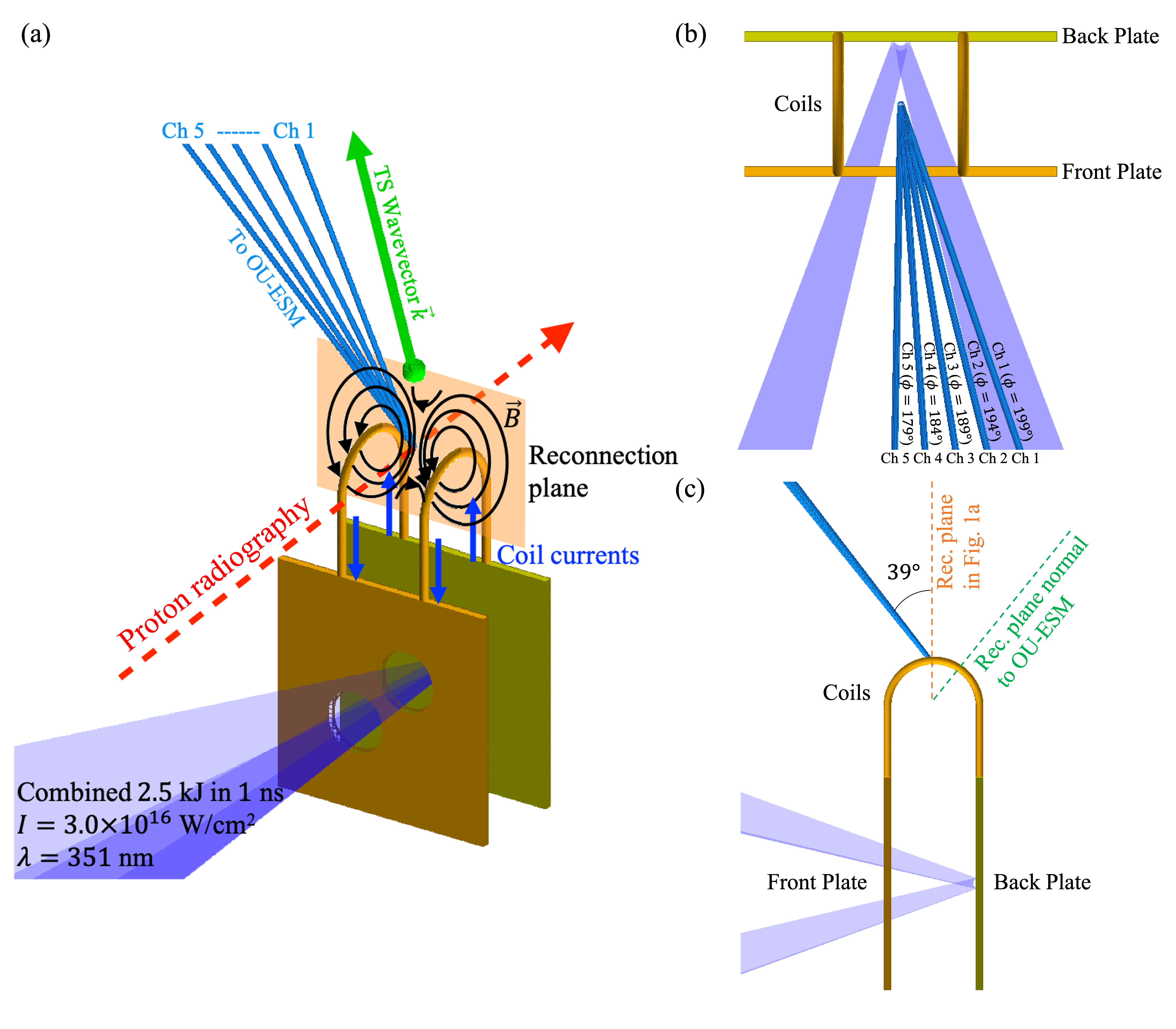
Our experiments using laser-powered capacitor coils were performed at the OMEGA EP facility at the Laboratory for Laser Energetics (LLE). The experimental setup, with diagnostic locations, is shown in Fig. 1. The capacitor-coil target is driven with two laser pulses, each delivering 1.25-kiloJoule of laser energy in a 1-ns square temporal profile at a wavelength of 351 nm. The corresponding on-target laser intensity is . Due to the laser interaction, strong currents are driven in the coils. In targets with two parallel coils, a magnetic reconnection field geometry is created between the coils, and in targets with one coil, a simple magnetic field around a wire is produced, representing a non-reconnection control case. Further information on capacitor coil target operation and design are provided in the Methods section.
The coil current profile can be approximated by a linear rise during the laser pulse (), followed by an exponential decay after laser turn-off. Target sheath normal acceleration (TNSA) Wilks et al. (2001) proton radiography measurements indicated a maximum coil current at of , corresponding to a magnetic field at the center of the coils of and an upstream reconnection magnetic field strength of , with a subsequent exponential decay time of Chien et al. (2019). During the current rise, the magnetic field strengthens, driving “push”-phase reconnection, where field lines are pushed into the reconnection region, and during current decay, “pull” reconnection occurs, where field lines are pulled out of the reconnection region Yamada et al. (1997). Due to the short timescale of the push phase relative to the pull phase, reconnection is driven more strongly during the push phase, and the push phase is the dominant source of particle acceleration.
We used Thomson scattering to diagnose the reconnecting copper plasma in a similar experiment on the OMEGA laser, and found electron density , ion density , and electron and ion temperatures . Due to the large , the ion plasma pressure is negligible compared to the electron plasma pressure, and the ratio of plasma pressure to magnetic pressure . The experiments are therefore firmly in the low- regime, most pertinent for particle acceleration in astrophysical conditions. The Lundquist number is , representing collisionless reconnection. The reconnection system size is defined by the inter-coil distance of , and when normalized by the ion skin depth , the normalized system size . Due to the small system size, the reconnection is deeply in the electron-only regime Phan et al. (2018), where ions are decoupled.
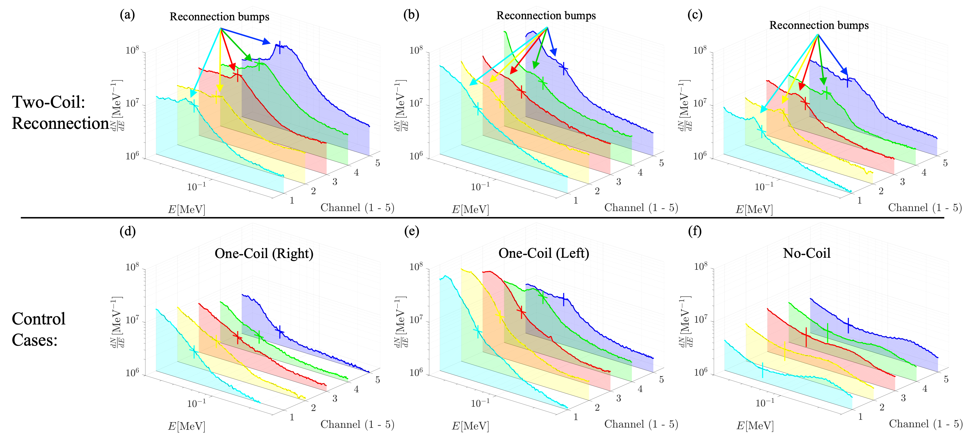
A time-integrated electron spectrometer – the Osaka University electron spectrometer (OU-ESM) – was used to measure the electron energy spectra. It is located away from the coils, at a polar angle of and scans an azimuthal range of with five equally-spaced detection channels. The OU-ESM channel orientation is shown in Fig. 1(b,c). Further details regarding the OU-ESM are given in the Methods section. Fig. 2 shows the experimentally measured OU-ESM data for three double-coil reconnection shots as well as two single-coil and one no-coil control shots. While neither one-coil nor no-coil shots represent perfect control cases, the combination of these configurations allows for better isolation of the reconnection signal.
Small differences in the laser energy profile and target properties among shots causes variations in otherwise nominally identical cases as seen in Fig. 2. However, focusing on the angular dependence across the channels for each shot reveals a key feature in the electron spectra: non-thermal “bumps” in the reconnection cases that do not appear in the control cases. The bumps span the range, and they are most pronounced at the near-normal Channel 5 () and weaken with increasing angle from normal. In contrast, the one-coil control cases do not exhibit consistent spectral bumps, and generally exhibit lower signal level. One exception is Figure 2e, which represents a one-coil shot with the coil on the left side (as viewed from the front of the target). Due to the coil magnetic field, low-energy electrons are deflected toward higher , resulting in an electron deficiency in Channel 5 and to a lesser extent, Channel 4. The no-coil control case exhibits an even lower signal level than the one-coil case: this is due to the lack of a magnetic field to deflect electrons toward the detector. The background “thermal” signal does not represent the plasma: it is the quasi-Maxwellian suprathermal distribution with a hot “temperature” of , created by laser-plasma instabilities (LPI), such as stimulated Raman scattering (SRS) and two-plasmon decay (TPD) Drake et al. (1984); Figueroa et al. (1984); Ebrahim et al. (1980).
These spectral bumps demonstrate non-thermal electron acceleration, and the detection angle dependence of the bump sizes suggests a directional anisotropy in the accelerated electron population. The strongest non-thermal population is seen in the direction out of the reconnection plane, anti-parallel to the reconnection electric field, indicating its responsibility for the direct acceleration Zenitani and Hoshino (2001); Uzdensky (2011); Cerutti et al. (2013).
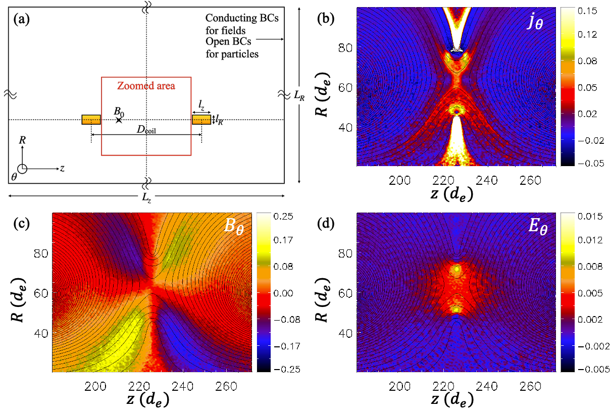
Interpretation of this particle acceleration mechanism is supported by particle-in-cell (PIC) simulations. We conducted 2-D cylindrical PIC simulations using the VPIC code Bowers et al. (2008) in order to model kinetic effects and simulated particle energy spectra (Fig. 3a shows the geometric setup). The -direction is the axis of symmetry, is the radial direction, and is the out-of-plane direction. Two rectangular-cross-section coils are placed in the simulation box, representing cross-sectional slices of the experimental U-shaped coils. Reconnection is driven by prescribing and injecting currents within the coils. We prioritize realistic mass ratio and in the simulation, at the expense of the reduced but scaled electron plasma frequency to electron gyrofrequency ratio, , due to the limited computational resources. Further details for the simulation setup are described in the Methods section.
The PIC simulation results demonstrate strong reconnection driven by the coil magnetic fields, with a typical out-of-plane quadrupole structure (Fig. 3c), indicative of scale separation between ions and electrons Uzdensky and Kulsrud (2006); Birn et al. (2001). In addition, a clear out-of-plane reconnection electric field is observed around the X-point, and the orientation of the electric field is consistent with push reconnection (see Fig. 3d).
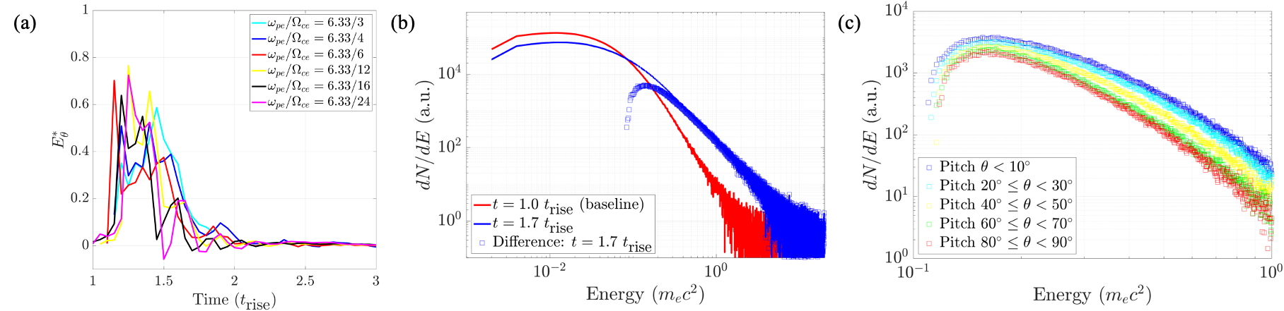
To obtain the reconnection rate, the reconnection electric field is typically normalized by an upstream , where is the upstream magnetic field strength and is the Alfvén velocity calculated with the ion density at the X-point. Figure 4a shows that the strongest reconnection occurs from , for all simulated values of . The diffusion time of the magnetic field through the plasma explains why this timing does not correspond to the expected period of push reconnection at . In nearly all cases, the reconnection rate reaches maximum values of , significantly higher than the typical rate expected for collisionless electron-ion reconnection Cassak, Liu, and Shay (2017): this is typical of electron-only reconnection, which is characterized by a normalized system size Sharma Pyakurel et al. (2019) .
Since the reconnection rate is constant across the scan, we estimate the reconnection electric field in physical units as , where the is the reconnection rate, as shown in Fig. 4a. Taking and a range of , . This value is consistent with fitting a power law of index to reconnection electric field strength as a function of .
| Low- plasma | Size (m) | (m-3) | (Tesla) | (eV) | (eV) | Notes or assumptions |
|---|---|---|---|---|---|---|
| Laser Plasma (this work) | 50 | Cu+18 plasma | ||||
| MagnetotailØieroset et al. (2002) | in-situ measurement | |||||
| Solar FlaresVilmer (2012); Raymond et al. (2012) | ||||||
| X-ray Binary Disk FlaresGoodman and Uzdensky (2008); Cangemi et al. (2021) | Cygnus X-3, , | |||||
| Crab Nebula FlaresKroon et al. (2016); Tavani et al. (2011); Abdo et al. (2011) | pair plasma | |||||
| Gamma Ray BurstsSari and Piran (1999); Uzdensky (2011) | pair plasma | |||||
| Magnetar FlaresBeloborodov (2017) | pair plasma, FRB 121102 | |||||
| AGN Disk FlaresTorricelli-Ciamponi, Pietrini, and Orr (2005); Goodman and Uzdensky (2008) | 4 | Seyfert 1 NGC 5548, , | ||||
| Radio LobesMassaro and Ajello (2011) | 0.1 | |||||
| Extragalactic JetsKataoka et al. (2003) | 3C 303 |
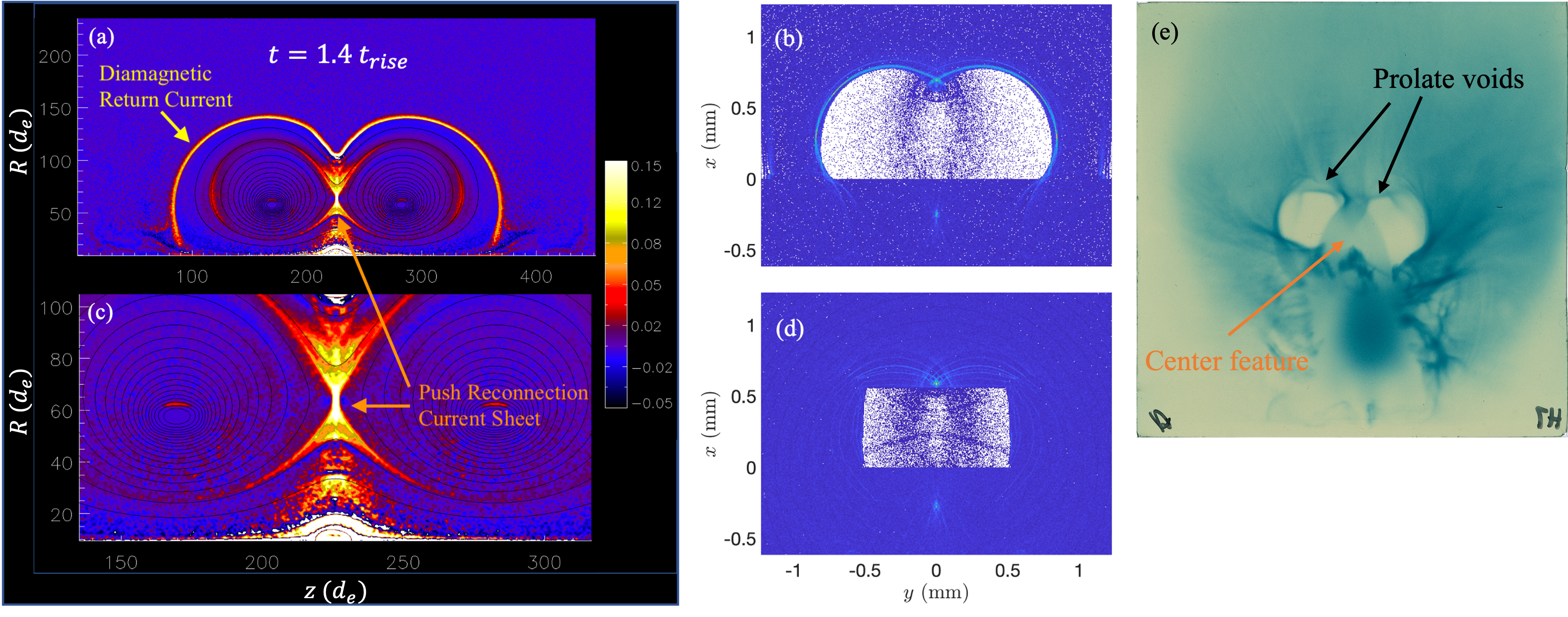
Electromagnetic fields from the PIC simulations are analyzed through a synthetic proton raytracing algorithm to predict a dark center feature corresponding to the reconnection current sheet during push reconnection. This center feature is observed in experimental proton radiographs taken at after the laser pulse (Fig. 5e), indicating the presence of reconnection in the experimental platform. To generate the synthetic proton radiograph, protons with kinetic energy of are advanced via a 4th-order Runge-Kutta algorithm. At each proton position, electromagnetic fields are inferred from the 2-D PIC fields, “swept” in angle along the semi-circular portion of the coils. More details of the synthetic raytracing algorithm are described in the Methods section.
Synthetic raytracing is performed for , corresponding to strong push reconnection. The center feature is reproduced in the radiograph (Fig. 5b), and two primary features in the out-of-plane current profiles (Fig. 5a) are potentially responsible for creating this center feature: the push reconnection current sheet and diamagnetic return current. To de-convolve the effects of each on the synthetic proton radiographs, raytracing is performed on a “zoomed” field, where the diamagnetic return current is largely shielded out (Fig. 5c). The center feature is maintained in this radiograph (Fig. 5d), indicating the source of the center feature as the push reconnection current sheet. Thus, the presence of a similar center feature in experimental radiographs is indicative of push reconnection and the corresponding electromagnetic fields.
Finally, the PIC simulations demonstrate non-thermal particle acceleration during the push phase of reconnection. Various filters are applied to the electron population to select the electrons that best compare to the experimental spectra. First, to focus on the electrons that are affected by reconnection, electrons are measured only within the zoomed-in simulation area shown in Fig. 3a. Second, the pitch angle is limited to select electrons that can escape and be measured by the OU-ESM detector. For our 2-D axisymmetric simulation, we do not limit the pitch angle, since for any fixed detector angle and pitch angle, a reconnection plane exists such that a particle accelerated from that plane would reach the detector.
Due to the particle injection scheme from , the baseline spectrum is taken at , in order to distinguish reconnection-accelerated electrons from injected electrons. The reconnection rate evolution shows that reconnection does not begin until , further validating this approach. Figure 4b shows the formation of a non-thermal electron tail. The tail grows larger with time, up to a maximum (at ), and begins to decay back to a Maxwellian, as reconnection stops and accelerated particles escape the system through the open boundaries. The time of the maximally non-thermal spectrum corresponds well to the reconnection electric field time dependence, demonstrating push reconnection as the source of the accelerated particles.
Comparison of the experimental particle spectra with PIC simulations supports acceleration by the reconnection electric field as the primary acceleration mechanism that forms the non-thermal electron tail. This is evidenced by the angular dependence and accelerated energies of the non-thermal tails in experimental measurements. The strongest non-thermal components are seen in Channel 5, corresponding to its near-normal orientation. The strength of the bump decreases as the azimuthal angle grows more oblique. Acceleration by the out-of-plane reconnection electric field would be expected to produce this angular dependence: electrons with larger pitch angles would be directed into regions with high field, resulting in re-magnetization, preventing the electron from reaching the detector. This angular dependence of the accelerated electrons is confirmed by PIC simulations, as shown in Fig. 4c, where non-thermal electrons decrease with increasing pitch angle from the reconnection electric field direction.
Other proposed acceleration mechanisms are not expected to be applicable because the required conditions for them are not satisfied in our experiment. Fermi acceleration typically requires multiple plasmoids in the current sheet as acceleration sites. Parallel electric field acceleration requires a finite guide field. Betatron acceleration requires increasing magnetic field in the downstream region. Polarization drift acceleration is not significant for electrons.
Although the accelerated particle spectrum from simulations could not be obtained for the experimental value of through scaling due to prohibitive computational cost (see Methods section), the simulation-determined scaling of the out-of-plane electric field is well-established. Using the calculated reconnection electric field , a simple estimate for the expected accelerated electron energy gain becomes , where is the electron charge, and is a characteristic acceleration distance, here taken to be . This predicts electrons, which represents an upper bound on accelerated electron energy with this mechanism, and is within a factor of 2 of the experimental bump of . Several potential factors can explain this discrepancy. First, a larger reconnection electric field and thus larger electron acceleration can be achieved with a larger than expected upstream magnetic field or a smaller than expected plasma density since . The former can occur due to magnetic field pileup in the upstream region. Plasma density near the X-point is uncertain because the Thomson scattering probes the plasma located in the downstream region above the coils.
Second, there is a possibility that the bump may not be due to reconnection: instead, due to the different magnetic topologies of the reconnection and one-coil cases, LPI-generated electrons of certain energies may be preferentially deflected toward certain angles, contributing to the observed spectral features. In the Supplementary Material section, this possibility is analyzed in detail using electron/positron raytracing with vacuum magnetic fields, and we conclude that this coil magnetic field deflection alone is unable to produce the experimental spectral trends and features observed. Plasma effects in the raytracing simulations are expected to be small, as illustrated by the low signal level in the no-coil electron spectra (Fig. 2f). By eliminating this alternative interpretation, this further supports that the detected electron spectral bump is due to reconnection.
The inference that direct electric field acceleration is operating in the experiments motivates estimating the corresponding attainable particle energies from this mechanism in representative low- collisionless reconnecting plasmas throughout the Universe Ji and Daughton (2011) and comparing to maximum inferred electron energies from observations. The result is shown in Table 1, where we have assumed that our experimental implications for the mostly electron-only reconnection regime can be extended to electron-ion or pair plasma reconnection regimes. This leads to the reconnection electric field typically found in collisionless reconnection Cassak, Liu, and Shay (2017). Therefore, the upper bound for the energy of the accelerated electrons by the reconnection electric field is established by the Hillas limit Hillas (1984) , where is a characteristic acceleration distance, here taken to be the system size .
The estimated maximum energy is within a factor of 2 for Earth’s magnetotail and Crab nebula flares, implying that if this mechanism is responsible for acceleration of the most energetic electrons in these two cases, coherent acceleration over a distance comparable to the system size is required. In all other cases, the observed maximum electron energy is well below the estimated theoretical maximum energy, suggesting that if this mechanism is at work, it must operate over length scales much shorter than the system size but with a properly distributed spread to populate the whole electron energy spectrum. Interestingly, this scaling of maximum energy has been also identified in large-scale simulations at low- but in relativistic regimes Guo et al. (2015).
Our laser-powered capacitor coils offer a unique experimental reconnection platform in magnetically driven low- plasmas to further study acceleration of electrons (and ions) in various reconnection regimes Ji and Daughton (2011); Ji et al. (2022) via direct detection of accelerated particles. The extent to which the same or different mechanisms Blandford et al. (2017); Guo et al. (2020) of particle acceleration emerge in different regimes will be of great interest to determine in future laboratory research and may depend on the particular reconnection boundary conditions and system geometries. Although no other mechanisms are excluded, our reported results serve as the first direct evidence of any hypothesized acceleration mechanism, by magnetic reconnection.
Methods
Laser-powered capacitor coil target
Laser-powered capacitor coil targets are composed of parallel plates (the capacitor) connected by one or multiple wires (the coils). Holes are formed in the front (facing the driving laser) plate to allow the laser beam(s) to bypass the front plate and only hit the back plate. Superthermal hot electrons are generated during the intense laser-solid interaction, some of which manage to escape from the back plate. A strong current is therefore supplied to the U-shaped wires from back to front, due to the resultant potential difference between the plates.
We use capacitor coil targets made from -thick copper. The capacitors are formed by two square parallel plates with length , with an inter-plate distance of . Two holes of radius are formed in the front plate to accommodate OMEGA EP long-pulse beams 3 and 4. The plates are joined by one or two parallel U-shaped coils, with rectangular cross-section . Each coil consists of two straight sections, joined by a semicircular section with radius . In two-coil targets, the coils are separated by . Capacitor coil targets are fabricated by laser-cutting a design in -thick sheet copper, then bending the coils into shape.
Particle spectra measurement using OU-ESM
The Osaka University electron spectrometer Habara et al. (2019) is a time-integrated diagnostic that can provide angular resolution in either polar or azimuthal angles, relative to the target. This is accomplished by the use of 5 channels, each separated in angle by . In the experiment, we chose the azimuthal angle spread, since this pitch angle allows for distinguishing between acceleration mechanisms in an axisymmetric setup, with symmetry in the polar direction.
After reaching the spectrometer, an electron first passes through a pinhole wide and deep. Separation of electron energies is accomplished with a set of permanent magnets placed along the detector line-of-sight, creating a magnetic field perpendicular to the line-of-sight. The force deflects differently-energized electrons different distances along the detector length onto a BAS-TR image plate. In general, impacts closer to the detector entrance represent lower-energy electrons. In the experiment, magnets were chosen corresponding to electron energies in the range.
The field of view and solid angle subtended by each channel are defined by the pinhole size , distance to target , and pinhole/collimator depth . The field of view is given by , which is significantly larger than the target size and sufficient to capture electrons from the main interaction. The solid angle is and provides the primary restriction for electrons reaching the detector.
The primary sources of error in interpreting OU-ESM data involve image plate response to energetic electrons and image plate scanning offsets. The image plate response is taken from Bonnet et al., 2013 Bonnet et al. (2013), and introduces a uncertainty. In addition, image plate signals decay with time, so image plates are scanned at exactly minutes after the shot for consistency in signal level. In interpreting the image plate, defining the edge of the magnets is critical to an accurate energy spectrum. Here, an uncertainty of approximately pixels, or is introduced, translating to an uncertainty in the spectrum energy.
Particle-in-cell simulation setup
The 2-D PIC simulation box has dimensions of and in the and directions, respectively, where is the inter-coil distance of . To avoid the difficult boundary at , a minimum radius of was used. Two rectangular-cross-section coils of width and height are located at and , matching experimental positions.
In the simulation, lengths are normalized to electron skin depth , and times are expressed in terms of the inverse electron plasma frequency . Due to the large Lundquist number, collisions are turned off in the simulation.
It is computationally untenable to perform a simulation with completely physical parameters, and so priorities must be made. An accurate particle spectrum is of great importance, so reducing ion-to-electron mass ratio is undesirable. In addition, the plasma has been shown to be a critical parameter in particle acceleration Li et al. (2018), so we maintain the physical in the simulation. To reduce computational time, we instead use artificially small values of the electron plasma frequency to electron gyrofrequency . By keeping constant, a reduced represents an artificially strong magnetic field, coupled to an artificially hot plasma. Scaling relations for electromagnetic field strength can be established as a function of in order to extrapolate to physical conditions. The physical , and simulations are run for reduced values , , , , , and .
Cell size is limited by the Debye length, so the number of cells changes with . At , the number of cells is , spanning . macro-particles of each species are initialized per cell. The achievable cell size and number of macro-particles per cell also limit a viable scaling of accelerated electron spectra to be established for the small electron diffusion region where electrons are demagnetized, and thus are free to be accelerated by the reconnection electric field.
For physical , the simulation is initialized with a uniform Maxwellian plasma with , to match experimental parameters. Compared to experiment, a lower initial plasma density is used due to the inclusion of a particle injection scheme from the coil region. A representative magnetic field strength is taken to be the upstream magnetic field at from the center between the coils. The simulation is therefore . Due to the artificially reduced values, ion and electron temperatures and coil magnetic fields are artificially increased, while keeping density constant to maintain plasma .
Electrically conducting boundary conditions are set for fields, and open boundary conditions Daughton, Scudder, and Karimabadi (2006) are set for particles in the and directions (periodic boundary conditions are set for ). The open boundary conditions prevent accelerated particles that would otherwise escape the system from being re-accelerated. Our choice therefore prevents an over-estimation of particle acceleration that would be inevitable with periodic or reflecting boundaries.
At , electromagnetic fields are set to 0. The capacitor coil currents are modeled by injecting currents with the following time profile:
| (1) |
where , , and match experimental measurements. Currents are oriented into the page ( direction). The coil magnetic fields are then calculated from the current distribution within the coils.
The reconnection plasma primarily emanates from the coils, due to ablation of copper plasma by Ohmic heating within the coils and irradiation by x-rays from the laser interaction. In contrast, the plasma generated at the laser spot takes a few nanoseconds to flow into the reconnection region, and does not play a significant role in reconnection, particularly during the push phase. To simulate the coil plasma, we use a particle injection scheme: a volume injector is implemented around the coils, with a Gaussian spatial profile (Gaussian width and height are set to and , respectively), and a linear time-dependence from . The injection rate is tuned to match experimental density measurements. Without the particle injection scheme, density voids form around the coils, as the strong magnetic field pressure pushes out plasma as the magnetic field diffuses outwards from the coils.
Proton raytracing using PIC electromagnetic fields
Protons are advanced through a 3-D representation of the PIC fields through a 4th-order Runge-Kutta algorithm. Electric and magnetic fields are applied onto a 3-D grid by projecting from a 2-D simulation using the following methodology:
-
1.
The center of the semi-circular coil is defined at the origin. For each proton near the coil region, the radius and azimuthal angle relative to the top-most point of the coil are calculated ( corresponds to the “vertical” reconnection plane).
-
2.
For angles corresponding to the lower hemisphere ( or ), electromagnetic fields are assumed to be .
-
3.
If the proton is far away enough from the coils to be outside the effective PIC simulation box ( or ), electromagnetic fields are assumed to be .
-
4.
The 3-D electric and magnetic fields corresponding to the radial and axial positions in the reconnection plane are found with linear interpolation.
-
5.
These fields are rotated by the azimuthal angle that corresponds to the proton location.
Simply, the 2-D reconnection plane is “swept” in angle along the semi-circular portion of the coils. For each synthetic radiograph, protons are sampled, with a maximum source angle of . The “impact coordinates” of each proton at a pre-defined synthetic detector are combined into a 2-D histogram, spanning in both directions with bins in each direction. Each bin thus represents a width.
Acknowledgements.
This work was supported by the LaserNetUS program and the High Energy Density Laboratory Plasma Science program by Office of Science, Fusion Energy Sciences (FES) and NNSA under Grant No. DE-SC0020103. The authors express their gratitude to General Atomics, the University of Michigan, and the Laboratory for Laser Energetics (LLE) for target fabrication, and to the OMEGA and OMEGA EP crews for experimental and technical support. The work was also supported by DOE Grant GR523126 and NSF Grant PHY-2020249.References
- Yamada, Kulsrud, and Ji (2010) M. Yamada, R. Kulsrud, and H. Ji, Rev. Mod. Phys. 82, 603 (2010).
- Ji et al. (2022) H. Ji, W. Daughton, J. Jara-Almonte, A. Le, A. Stanier, and J. Yoo, “Magnetic reconnection in the era of exascale computing and multiscale experiments,” in press, Nat. Rev. Phys. (2022).
- Blandford et al. (2017) R. Blandford, Y. Yuan, M. Hoshino, and L. Sironi, Space Science Rev. 207, 291 (2017).
- Guo et al. (2020) F. Guo, Y.-H. Liu, X. Li, H. Li, W. Daughton, and P. Kilian, Phys. Plasmas 27, 080501 (2020).
- Masuda et al. (1994) S. Masuda, T. Kosugi, H. Hara, S. Tsuneta, and Y. Ogawara, Nature 371, 495 (1994).
- Øieroset et al. (2002) M. Øieroset, R. P. Lin, T. D. Phan, D. E. Larson, and S. D. Bale, Phys. Rev. Lett. 89, 195001 (2002).
- Krucker et al. (2010) S. Krucker, H. S. Hudson, L. Glesener, S. M. White, S. Masuda, J.-P. Wuelser, and R. P. Lin, Astrophys. J. 714, 1108 (2010).
- Abdo et al. (2011) A. Abdo, M. Ackermann, M. Ajello, A. Allafort, L. Baldini, J. Ballet, G. Barbiellini, D. Bastieri, K. Bechtol, and R. Bellazzini, Science 331, 739 (2011).
- Tavani et al. (2011) M. Tavani, A. Bulgarelli, V. Vittorini, A. Pellizzoni, E. Striani, P. Caraveo, M. Weisskopf, A. Tennant, G. Pucella, and A. Trois, Science 331, 736 (2011).
- Chen et al. (2020) B. Chen, C. Shen, D. E. Gary, K. K. Reeves, G. D. Fleishman, S. Yu, F. Guo, S. Krucker, J. Lin, G. M. Nita, and X. Kong, Nature Astronomy 4, 1140 (2020).
- Drenkhahn and Spruit (2002) G. Drenkhahn and H. C. Spruit, Astro. Astrophys. 391, 1141 (2002).
- Sironi and Spitkovsky (2014) L. Sironi and A. Spitkovsky, Astrophys. J. Lett. 783, L21 (2014).
- Werner et al. (2016) G. R. Werner, D. A. Uzdensky, B. Cerutti, K. Nalewajko, and M. C. Begelman, Astrophys. J. Lett. 816, L8 (2016).
- Li et al. (2017) X. Li, F. Guo, H. Li, and G. Li, Astrophys. J. 843, 21 (2017).
- Dahlin (2020) J. T. Dahlin, Phys. Plasmas 27, 100601 (2020).
- Drake et al. (2006) J. F. Drake, M. Swisdak, H. Che, and M. A. Shay, Nature 443, 553 (2006).
- Hoshino et al. (2001) M. Hoshino, T. Mukai, T. Terasawa, and I. Shinohara, J. Geophys. Res. 106, 25979 (2001).
- Egedal, Le, and Daughton (2013) J. Egedal, A. Le, and W. Daughton, Phys. Plasmas 20, 061201 (2013).
- Zenitani and Hoshino (2001) S. Zenitani and M. Hoshino, Astrophys. J. Lett. 562, L63 (2001).
- Gao et al. (2016) L. Gao, H. Ji, G. Fiksel, W. Fox, M. Evans, and N. Alfonso, Physics of Plasmas 23, 043106 (2016).
- Chien et al. (2019) A. Chien, L. Gao, H. Ji, Y. Xiaoxia, E. Blackman, H. Chen, P. Efthimion, G. Fiksel, D. Froula, K. Hill, K. Huang, Q. Lu, J. Moody, and P. Nilson, Physics of Plasmas 26, 062113 (2019).
- Chien et al. (2021) A. Chien, L. Gao, S. Zhang, H. Ji, E. Blackman, H. Chen, G. Fiksel, K. Hill, and P. Nilson, Phys. Plasmas 28, 052105 (2021).
- Uzdensky (2011) D. Uzdensky, “Magnetic reconnection in extreme astrophysical environments,” (2011), published in Space Sci. Rev., DOI: 10.1007/s11214-011-9744-5.
- Cerutti et al. (2013) B. Cerutti, G. R. Werner, D. A. Uzdensky, and M. C. Begelman, Astrophys. J. 770, 147 (2013).
- Kroon et al. (2016) J. J. Kroon, P. A. Becker, J. D. Finke, and C. D. Dermer, Astrophys. J. 833, 157 (2016).
- Dahlin, Drake, and Swisdak (2014) J. T. Dahlin, J. F. Drake, and M. Swisdak, Physics of Plasmas 21, 092304 (2014), https://doi.org/10.1063/1.4894484 .
- Dahlin, Drake, and Swisdak (2016) J. T. Dahlin, J. F. Drake, and M. Swisdak, Physics of Plasmas 23, 120704 (2016), https://doi.org/10.1063/1.4972082 .
- Totorica, Abel, and Fiuza (2016) S. R. Totorica, T. Abel, and F. Fiuza, Phys. Rev. Lett. 116, 095003 (2016).
- Savrukhin (2001) P. V. Savrukhin, Physical Review Letters 86, 3036 (2001).
- Klimanov et al. (2007) I. Klimanov, A. Fasoli, T. P. Goodman, and the TCV team, Plasma Physics and Controlled Fusion 49, L1 (2007).
- DuBois et al. (2017) A. M. DuBois, A. F. Almagri, J. K. Anderson, D. J. Den Hartog, J. D. Lee, and J. S. Sarff, Phys. Rev. Lett. 118, 075001 (2017).
- Nilson et al. (2006) P. M. Nilson, L. Willingale, M. C. Kaluza, C. Kamperidis, S. Minardi, M. S. Wei, P. Fernandes, M. Notley, S. Bandyopadhyay, M. Sherlock, R. J. Kingham, M. Tatarakis, Z. Najmudin, W. Rozmus, R. G. Evans, M. G. Haines, A. E. Dangor, and K. Krushelnick, Phys. Rev. Lett. 97, 255001 (2006).
- Willingale et al. (2010) L. Willingale, P. M. Nilson, M. C. Kaluza, A. E. Dangor, R. G. Evans, P. Fernandes, M. G. Haines, C. Kamperidis, R. J. Kingham, C. P. Ridgers, M. Sherlock, A. G. R. Thomas, M. S. Wei, Z. Najmudin, K. Krushelnick, S. Bandyopadhyay, M. Notley, S. Minardi, M. Tatarakis, and W. Rozmus, Phys. Plasmas 17, 043104 (2010).
- Zhong et al. (2010) J. Zhong, Y. Li, X. Wang, J. Wang, Q. Dong, C. Xiao, S. Wang, X. Liu, L. Zhang, L. An, F. Wang, J. Zhu, Y. Gu, X. He, G. Zhao, and J. Zhang, Nature Phys. 6, 984 (2010).
- Fiksel et al. (2014) G. Fiksel, W. Fox, A. Bhattacharjee, D. H. Barnak, P. Y. Chang, K. Germaschewski, S. X. Hu, and P. M. Nilson, Phys. Rev. Lett. 113, 105003 (2014).
- E Raymond et al. (2018) A. E Raymond, C. Dong, A. Mckelvey, C. Zulick, N. Alexander, A. Bhattacharjee, P. T Campbell, H. Chen, V. Chvykov, E. Del Rio, P. Fitzsimmons, W. Fox, B. Hou, A. Maksimchuk, C. Mileham, J. Nees, P. M Nilson, C. Stoeckl, A. Thomas, and L. Willingale, Physical Review E 98, 043207 (2018).
- Dong et al. (2012) Q.-L. Dong, S.-J. Wang, Q.-M. Lu, C. Huang, D.-W. Yuan, X. Liu, X.-X. Lin, Y.-T. Li, H.-G. Wei, J.-Y. Zhong, J.-R. Shi, S.-E. Jiang, Y.-K. Ding, B.-B. Jiang, K. Du, X.-T. He, M. Y. Yu, C. S. Liu, S. Wang, Y.-J. Tang, J.-Q. Zhu, G. Zhao, Z.-M. Sheng, and J. Zhang, Phys. Rev. Lett. 108, 215001 (2012).
- Zhong et al. (2016) J. Y. Zhong, J. Lin, Y. T. Li, X. Wang, Y. Li, K. Zhang, D. W. Yuan, Y. L. Ping, H. G. Wei, J. Q. Wang, L. N. Su, F. Li, B. Han, G. Q. Liao, C. L. Yin, Y. Fang, X. Yuan, C. Wang, J. R. Sun, G. Y. Liang, F. L. Wang, Y. K. Ding, X. T. He, J. Q. Zhu, Z. M. Sheng, G. Li, G. Zhao, and J. Zhang, The Astrophysical Journal Supplement Series 225, 30 (2016).
- Wilks et al. (2001) S. C. Wilks, A. B. Langdon, T. E. Cowan, M. Roth, M. Singh, S. Hatchett, M. H. Key, D. Pennington, A. MacKinnon, and R. A. Snavely, Physics of Plasmas 8, 542 (2001).
- Yamada et al. (1997) M. Yamada, H. Ji, S. Hsu, T. Carter, R. Kulsrud, N. Bretz, F. Jobes, Y. Ono, and F. Perkins, Physics of Plasmas 4, 1936 (1997).
- Phan et al. (2018) T. D. Phan, J. P. Eastwood, M. A. Shay, J. F. Drake, B. U. Ö. Sonnerup, M. Fujimoto, P. A. Cassak, M. Øieroset, J. L. Burch, R. B. Torbert, A. C. Rager, J. C. Dorelli, D. J. Gershman, C. Pollock, P. S. Pyakurel, C. C. Haggerty, Y. Khotyaintsev, B. Lavraud, Y. Saito, M. Oka, R. E. Ergun, A. Retino, O. Le Contel, M. R. Argall, B. L. Giles, T. E. Moore, F. D. Wilder, R. J. Strangeway, C. T. Russell, P. A. Lindqvist, and W. Magnes, Nature 557, 202 (2018).
- Drake et al. (1984) R. P. Drake, R. E. Turner, B. F. Lasinski, K. G. Estabrook, E. M. Campbell, C. L. Wang, D. W. Phillion, E. A. Williams, and W. L. Kruer, Phys. Rev. Lett. 53, 1739 (1984).
- Figueroa et al. (1984) H. Figueroa, C. Joshi, H. Azechi, N. A. Ebrahim, and K. Estabrook, The Physics of Fluids 27, 1887 (1984), https://aip.scitation.org/doi/pdf/10.1063/1.864801 .
- Ebrahim et al. (1980) N. A. Ebrahim, H. A. Baldis, C. Joshi, and R. Benesch, Phys. Rev. Lett. 45, 1179 (1980).
- Bowers et al. (2008) K. J. Bowers, B. J. Albright, L. Yin, B. Bergen, and T. J. T. Kwan, Phys. Plasmas 15, 055703 (2008).
- Uzdensky and Kulsrud (2006) D. Uzdensky and R. Kulsrud, Phys. Plasmas 13, 062305 (2006).
- Birn et al. (2001) J. Birn, J. Drake, M. Shay, B. Rogers, R. Denton, M. Hesse, M. Kuznetsova, Z. Ma, A. Bhattachargee, A. Otto, and P. Pritchett, J. Geophys. Res. 106, 3715 (2001).
- Cassak, Liu, and Shay (2017) P. Cassak, Y.-H. Liu, and M. Shay, J. Plasma Phys. 83, 715830501 (2017).
- Sharma Pyakurel et al. (2019) P. Sharma Pyakurel, M. A. Shay, T. D. Phan, W. H. Matthaeus, J. F. Drake, J. M. TenBarge, C. C. Haggerty, K. G. Klein, P. A. Cassak, T. N. Parashar, M. Swisdak, and A. Chasapis, Physics of Plasmas 26, 082307 (2019), https://doi.org/10.1063/1.5090403 .
- Ji and Daughton (2011) H. Ji and W. Daughton, Phys. Plasmas 18, 111207 (2011).
- Vilmer (2012) N. Vilmer, Philosophical Transactions of the Royal Society of London Series A 370, 3241 (2012).
- Raymond et al. (2012) J. C. Raymond, S. Krucker, R. P. Lin, and V. Petrosian, Space Science Rev. 173, 197 (2012).
- Goodman and Uzdensky (2008) J. Goodman and D. Uzdensky, Astrophys. J. 688, 555 (2008).
- Cangemi et al. (2021) F. Cangemi, J. Rodriguez, V. Grinberg, R. Belmont, P. Laurent, and J. Wilms, Astro. Astrophys. 645, A60 (2021).
- Sari and Piran (1999) R. Sari and T. Piran, Astrophys. J. 520, 641 (1999).
- Beloborodov (2017) A. M. Beloborodov, Astrophys. J. 843, L26 (2017).
- Torricelli-Ciamponi, Pietrini, and Orr (2005) G. Torricelli-Ciamponi, P. Pietrini, and A. Orr, Astro. Astrophys. 438, 55 (2005).
- Massaro and Ajello (2011) F. Massaro and M. Ajello, Astrophys. J. Lett. 729, L12 (2011).
- Kataoka et al. (2003) J. Kataoka, P. Edwards, M. Georganopoulos, F. Takahara, and S. Wagner, Astro. Astrophys. 399, 91 (2003).
- Hillas (1984) A. M. Hillas, Annual Review of Astronomy and Astrophysics 22, 425 (1984), https://doi.org/10.1146/annurev.aa.22.090184.002233 .
- Guo et al. (2015) F. Guo, Y.-H. Liu, W. Daughton, and H. Li, Astrophys. J. 806, 1 (2015).
- Habara et al. (2019) H. Habara, T. Iwawaki, T. Gong, M. S. Wei, S. T. Ivancic, W. Theobald, C. M. Krauland, S. Zhang, G. Fiksel, and K. A. Tanaka, Review of Scientific Instruments 90, 063501 (2019), https://doi.org/10.1063/1.5088529 .
- Bonnet et al. (2013) T. Bonnet, M. Comet, D. Denis-Petit, F. Gobet, F. Hannachi, M. Tarisien, M. Versteegen, and M. M. Aléonard, Review of Scientific Instruments 84, 103510 (2013), https://doi.org/10.1063/1.4826084 .
- Li et al. (2018) X. Li, F. Guo, H. Li, and J. Birn, The Astrophysical Journal 855, 80 (2018).
- Daughton, Scudder, and Karimabadi (2006) W. Daughton, J. Scudder, and H. Karimabadi, Physics of Plasmas 13, 072101 (2006), https://doi.org/10.1063/1.2218817 .
Supplemental Material
Study on LPI-generated electron deflections by coil magnetic fields
The angular dependence of accelerated electrons measured by OU-ESM was interpreted as evidence of electrons accelerated by the reconnection electric field. However, this interpretation does not take into account the possibility of LPI-generated electrons being deflected by coil magnetic fields preferentially in certain angles, resulting in the measured angular distribution in the electron energy spectra. To explore this possibility, numerical raytracing is performed using positrons advanced through the vacuum coil magnetic field.
Instead of advancing electrons from the laser spot to the electron spectrometer, positrons are initialized at the spectrometer, and advanced toward the capacitor-coil target. Due to charge-parity-time (CPT) symmetry, a positron advancing “backward” in time through electromagnetic fields is equivalent to an electron advancing “forward” in time through the same fields. These two simulations are thus functionally similar, but the former allows for significantly faster computation times due to more limited angular spread around the collimator at the OU-ESM. Positron raytracing is performed for all OU-ESM channels. Positrons with kinetic energy are initialized at the entrance of each channel, with an angular spread of in both polar and azimuthal angles, providing a field of view that adequately encompasses the entire capacitor coil target. These positrons are then advanced through the vacuum magnetic fields calculated from the coil current geometry via a 4th-order Runge-Kutta algorithm. The majority of these positrons leave the field region, but the few that impact the capacitor coil plates are recorded. In addition to scanning across the OU-ESM channel angles, the raytracing is scanned across various coil currents, from , up to the maximum coil current of , and 3 different coil configurations: double coil (reconnection), left coil only (control), and right coil only (control). For each combination of OU-ESM channel, coil current, and coil configuration, positrons are used.
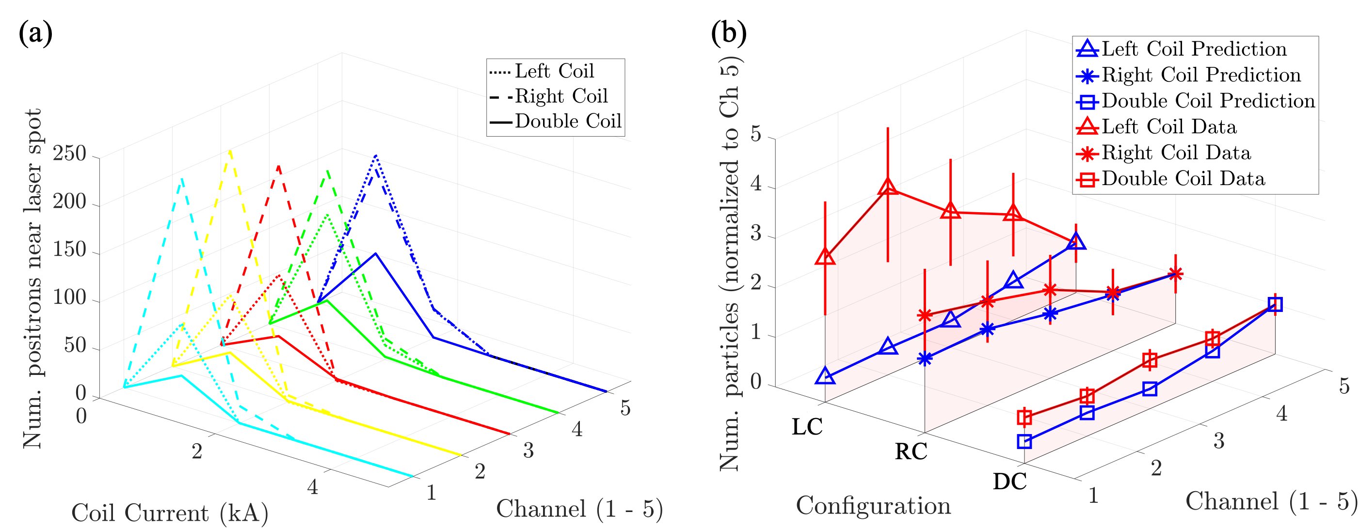
In all coil configurations, positrons are only deflected toward the laser spot (defined as a -radius circle centered on the back plate) for small finite coil currents . For larger coil currents (), the positrons are deflected completely away from the back plate, with no deposited positrons recorded. For , the deposition pattern of positrons is seen to move “downward” with increasing coil current. This is explained by the force from the “horizontal” magnetic field (left to right in Fig. 1b).
An interesting trend appears when comparing the double coil reconnection configurations with either right or left coil control configurations. Across all channels, the right and left coil configurations (represented by triangle and asterisk markers, respectively) result in more positrons deflected near the laser spot than the double coil configuration (represented by square markers). Reverting to the electron frame, this implies that LPI-generated electrons with energies of are less likely to be deflected toward the electron spectrometer by double coil configurations, compared to single coil configurations. The possibility of the double coil case acting as an “energy selector” causing the spectral bumps is therefore small. Furthermore, we have shown that electrons are deflected toward the OU-ESM for a very limited range of coil currents, when compared to the maximum coil current of . As OU-ESM is a time-integrated diagnostic, even if some sort of energy selection mechanism were to exist, the effect on the entire spectrum would be small, as the coil current spends comparatively little time in the range.
The model is not perfect, primarily due to the assumption of vacuum magnetic fields and the ignoring of plasma effects. The relative importance of plasma effects in the exercise can be illustrated by the no-coil experimental spectra shown in Fig. 2f. Without plasma effects, no LPI electrons are expected at the OU-ESM, as the field of view of the instrument do not include the laser spot, from which LPI electrons originate. The low signal level of the measured no-coil spectra therefore illustrates the relative insignificance of plasma effects on measured and simulated electron spectra. Despite the assumptions, the exercise overall does not support an energy selection mechanism, whereby LPI-generated electrons of energy are deflected by coil magnetic fields alone and are responsible for the spectral bump.
Inter-channel trends can also be predicted by the raytracing exercise, and compared to experimental values. For instance, Fig. 6a shows an increase in double coil signal with increasing channel. These LPI-only predictions can be established for all three configurations for coil current . Similarly, experimental signal levels for electron energy can be compared across channels for these three configurations. The results are summarized in Fig. 6b. The double coil experimental ratios roughly agree with the LPI-only predicted values, hovering close to a ratio of unity, when compared to Channel 5. The right coil configuration shows agreement between LPI-predicted and experimental trends, helped by large error bars in the data. The left coil data, however, demonstrates a large deviation from raytracing predictions. This inconsistency shows that the experimental results cannot be adequately explained with vacuum magnetic fields alone deflecting electrons toward different detector channels.