Direct interpolative construction of the discrete Fourier transform as a matrix product operator
Abstract
The quantum Fourier transform (QFT), which can be viewed as a reindexing of the discrete Fourier transform (DFT), has been shown to be compressible as a low-rank matrix product operator (MPO) or quantized tensor train (QTT) operator [1]. However, the original proof of this fact does not furnish a construction of the MPO with a guaranteed error bound. Meanwhile, the existing practical construction of this MPO, based on the compression of a quantum circuit, is not as efficient as possible. We present a simple closed-form construction of the QFT MPO using the interpolative decomposition, with guaranteed near-optimal compression error for a given rank. This construction can speed up the application of the QFT and the DFT, respectively, in quantum circuit simulations and QTT applications. We also connect our interpolative construction to the approximate quantum Fourier transform (AQFT) by demonstrating that the AQFT can be viewed as an MPO constructed using a different interpolation scheme.
1 Introduction
The quantum Fourier transform (QFT) [2] is one of the most important algorithmic primitives in quantum computing. It is often viewed as providing exponential speedup compared to the fast Fourier transform (FFT), due to its gate complexity of acting on an -qubit quantum state. Such a state can be viewed as an -dimensional vector with , and under this identification the QFT corresponds to a discrete Fourier transform (DFT), which costs operations via the FFT.
However, if one makes use of low-rank structure of the input state, the QFT can often be simulated classically using efficient operations with matrix product states (MPS) and matrix product operators (MPO) [3, 4, 5, 6, 7]. Equivalently, the DFT of functions compressible as quantized tensor trains (QTT) [8, 9] can be computed with exponential speedup. For example, one can remove the long-range quantum gates in the QFT circuit that are close to identity, resulting in the approximate QFT (AQFT) [10]. The AQFT automatically admits an MPO representation due to the bounded interaction length of the circuit [11, 12, 13], and therefore it can be simulated classically on any input states represented as an MPS. The full QFT circuit can also be viewed as the composition of MPOs of rank 2, which can be applied sequentially to MPS inputs with intermediate compressions [14, 15]. This approach has been called the “superfast Fourier transform” or QTT-FFT [15]. Recently, the entire QFT operator was proven to be compressible as an MPO [1]. In practice, the MPO representation of the QFT, referred to as the QFT MPO, can be obtained by contracting and compressing the entire QFT circuit. Interestingly, for a given error tolerance, the QFT MPO was observed to have smaller ranks compared to the AQFT MPO [1, 16], implying that the long-range gates actually play a role in reducing the entanglement.
Classical simulation of the QFT can be used as a classical algorithm that outperforms the FFT in restricted settings. Concretely, one converts an -dimensional vector into an -site MPS and contracts it with the QFT circuit or the QFT MPO. In this approach, even if the state admits compression as an MPS, the conversion dominates the time complexity if the state is formed as a dense vector and compressed via the TT singular value decomposition (TT-SVD) [8]. A randomized variant of TT-SVD yields an speed-up [1], and other heuristic approaches such as TT-cross [17, 18] can yield speedup, enabling the QTT-FFT of [15]. If the input vector is the quantized representation of a function that is well approximated in a multiresolution polynomial basis, a direct analytical construction based on the interpolative decomposition can be applied with quantitative control over the error [19]. The interpolating cores introduced in [19] are an essential ingredient in this work. In some situations, the input is automatically available in low-rank tensor format, such as the evolving state of a differential equation solved within the QTT format [20, 21, 22, 23] or a quantum simulation solved using an MPS representation of the state [24, 25, 26].
In these applications, an efficient and accurate construction of the QFT MPO is crucial. While it can be constructed efficiently by contracting the QFT circuit, this approach has a few drawbacks. First, to avoid exponential scaling in , one must perform intermediate compressions before the final MPO is formed, and no rigorous a priori estimate of the accumulated error is available, even though the approach is highly accurate in practice and heuristic arguments support its accuracy. Second, the circuit contraction takes time, where is the bond dimension, while the MPO ultimately contains at most information, so the computational complexity does not appear to be optimal, as we confirm in this work. Third, the parameters in the circuit decay like , so for large we unavoidably lose accuracy in the long-range gates due to the limitations of numerical precision. This loss of accuracy resembles the approximation imposed by the AQFT circuit, which increases the bond-dimension by the aforementioned observation in [1, 16].
In this paper, we present a simple closed-form construction of the QFT MPO, avoiding circuit contraction and eliminating all three drawbacks mentioned above. The construction involves an interpolative decomposition based on polynomial interpolation on the Chebyshev-Lobatto grid, applied recursively on each qubit, and yields a nearly optimal MPO compression for a given bond dimension. The bond dimension of the construction corresponds to the number of interpolation points. For a fixed number of qubits, the error decreases super-exponentially with respect to the bond dimension, matching the bounds for the Schmidt coefficients derived in [1]. Furthermore, the tensor cores are all identical (excepting the first and last). Finally, we show that the AQFT circuit can also be interpreted as an MPO constructed in the same fashion but with a different interpolation scheme, i.e., piecewise constant interpolation. This interpolation scheme converges more slowly with respect to the number of interpolation points, explaining the observation that the AQFT has a higher MPO rank than the QFT MPO, for a given error tolerance.
We outline the paper as follows. In Section 2 we present some preliminary definitions and notation. In Section 3 we demonstrate how the interpolative decomposition yields a rank bound for the unfolding matrices of the QFT, similar to that of [1]. (In fact, our rank bound is not implied by [1] since it is defined in terms of the infinity norm error, rather than the Frobenius norm error.) We also describe the connection of the rank bound for the unfolding matrices with the complementary low-rank structure [27] that has been observed for the DFT and other operators. This section can also be viewed as a warm-up for Section 4, in which we present our construction of the QFT as an MPO using the interpolative decomposition. In Section 5, we bound the error of this construction. In Section 6, we illustrate the connection to the AQFT.
1.1 Acknowledgments
The authors are grateful to Sandeep Sharma, Garnet Chan, and Yuehaw Khoo for helpful discussions.
2 Preliminaries
Consider discrete indices , where , and define the matrix of the discrete Fourier transform (DFT)
We comment that in the quantum computing literature, the convention for the QFT is rather than , but we use the latter to match the standard definition of the DFT.
We can place and , respectively, in bijection with bit strings and in via
| (2.1) |
These bits can be viewed as binary digits for and with opposite orderings.
Then we can view as a tensor of size via this identification:
| (2.2) |
In the QFT, and correspond to the input and output indices of the -th qubit respectively. Notice that is the least significant bit while is the most significant bit, and it is a key point in [1] that only this ordering induces low-rank structure of the QFT as a matrix product operator or quantized tensor train operator, which is defined as the approximate factorization
| (2.3) |
where we used the notation . The integers are often called the bond dimensions or TT ranks, and for simplicity we assume that for some fixed . The tensors are referred to as tensor cores.
We also define the -th unfolding matrix of as the matrix
| (2.4) |
where we view the multi-indices before and after the semicolon, respectively, as row and column indices of a matrix. It is shown in [8] that a QTT with good approximation exists if the -th unfolding matrix is numerically low-rank for all .
To measure the error of our decompositions it is useful to define a tensor infinity norm
| (2.5) |
as the largest magnitude of any element of the tensor. We will use this notation for tensors of different shapes, but ultimately the accuracy of our MPO approximation itself is most naturally expressed in this norm.
We also define notations for our interpolation scheme. We will denote the Chebyshev-Lobatto grid points (shifted and scaled to the interval ) by
| (2.6) |
for . Throughout, we use to denote grid size (or more properly, the grid size minus one). The corresponding Chebyshev-Lobatto interpolation of a function , i.e., the Lagrange polynomial interpolation on the Chebyshev-Lobatto grid, is
| (2.7) |
where the are degree- polynomials such that , i.e., the Lagrange interpolating polynomials for this grid. In the case of Chebyshev-Lobatto interpolation, the are sometimes called the Chebyshev cardinal functions, which can be evaluated directly with simple trigonometric formulas [28], bypassing the application of the more general formula for Lagrange basis functions.
3 Rank bound
Although the rank of as an MPO was already bounded in [1], we provide an alternative rank bound from an interpolative perspective. In fact, this point of view yields entrywise control over the error of , which is not captured by the bounds on the Schmidt spectrum in [1].
Our motivation arises from computing
Now if and , then , and therefore
It follows that we can write
where we have overloaded the notation for slightly to denote the quantized tensor representations of DFT matrices of arbitrary sizes.
It is then useful to define
| (3.1) |
so
| (3.2) |
Then we are motivated to consider, for arbitrary , the function
We can approximate with Chebyshev-Lobatto interpolation to obtain
If this equality holds with pointwise error bounded by , then the rank- approximation of the -th unfolding matrix of has entrywise error bounded by .
The above arguments are reviewed diagrammatically in Fig. 3.1. Next we state and prove an error bound.
Proposition 1.
There exists a rank- approximation of the -th unfolding matrix of whose entrywise error is bounded uniformly by
Remark 2.
This bound on the infinity norm error implies a bound on the Frobenius norm error very similar to the Frobenius error implied by the Schmidt coefficient bound in [1], but with a worse exponential prefactor . However, the decay present in both bounds quickly takes over. Thus Proposition 1 has similar implications as the main theorem in the context of [1]. Meanwhile, if entrywise control is needed, then Proposition 1 has additional value.

Proof of Proposition 1.
To apply standard results on Chebyshev interpolation error, we rescale to the reference interval , defining
Note that extends analytically to all of . For , define the Bernstein ellipse by
where
Moreover, , so on the Bernstein ellipse we have that
Then by Theorem 8.2 of [29], it follows that the pointwise error of Chebyshev interpolation of is bounded (independently of ) by
for any . We want to choose to optimize this bound. It is roughly equivalent to find the optimizer of the numerator, which is simple to compute exactly as . Then plugging into our expression yields the bound
which completes the proof. ∎
3.1 Connection to complementary low-rankness
The low-rankness of the unfolding matrices in fact implies the well-known complementary low-rank property [27] of the DFT matrix. This property says that, if we partition the matrix into blocks of size where is the level of the partition, then for all levels each block is numerically low-rank. For example, when , the partition can be visualized as follows.
![[Uncaptioned image]](https://cdn.awesomepapers.org/papers/46479463-3c9c-4478-a742-2892a4a7be4f/x2.png)
We argue that the low-rankness of the unfolding matrix is a stronger property than complementary low-rankness. Suppose that we fix the level and let denote the -th block of the DFT matrix at this level. The complementary low-rank property implies that a decomposition exists for all , i.e., for some tensors and . On the other hand, the low-rankness of the unfolding matrix implies the more special structure .
We illustrate this point diagrammatically as follows.
![[Uncaptioned image]](https://cdn.awesomepapers.org/papers/46479463-3c9c-4478-a742-2892a4a7be4f/x3.png)
Here depicts the partition and the block indices for and , and describes the low-rank approximation of the unfolding matrix, which is equivalent to . It is indeed known [30] that the submatrices for the DFT can be written as where (resp., ) is the unitary diagonal matrix generated by the -th (resp., -th) column of the (resp., ) DFT. This point is essentially a restatement of (3.2).
4 Direct interpolative construction
The preceding argument does not directly furnish an approximate presentation of as an MPO. Now we turn to the task of such a construction, which is illustrated diagrammatically in Fig. 4.1.

Recall our definition (3.1) for in terms of the bit substring , which we reproduce here as
for every . Note that for all , and moreover we can construct the sequence recursively via the relation
which holds for . Note that .
We will construct inductively a sequence of tensors , , with entries specified by
| (4.1) |
where we point out that is always understood to be implicitly defined in terms of .
For the base case, the tensor can be written explicitly
Alternatively, we may view for each as the matrix
Moreover, we can obtain our target as
under the convention that is the index of the leftmost node .
Then we claim that can be obtained approximately from by attaching a single tensor core on the right. To see this, expand:
Now for any , observe that , so the second factor in the last expression is just . Moreover, we can substitute in the third factor and in the last factor to obtain
where we retain our definition of from the last section.
Then we can insert an interpolative decomposition
| (4.2) |
into our expression for , yielding
where we have defined the tensor core via
| (4.3) |
Alternatively we can write
Then we have argued that we can approximate as an MPO with leftmost core , internal cores , and rightmost core given by
| (4.4) |
Since for all , we can neatly express the leftmost core in terms of as
| (4.5) |
Remark 3.
It is straightforward to extend the scheme to qudits. Redefining and to be elements of , we consider the -ary expansions
in place of (2.1).
In this setting the DFT matrix can be written as
Following the same construction, we obtain the core
5 Error bound
The following result bounds the entrywise error of the MPO constructed as above.
Theorem 4.
For fixed integer , let denote the -site, rank- MPO comprised of internal cores
leftmost core and rightmost core , as described in the preceding discussion and illustrated in Figure 4.1(c).
Then the entrywise error of this MPO with respect to the true DFT operator is bounded as
where is the Lebesgue constant of -point Chebyshev-Lobatto interpolation and is the worst case -point Chebyshev-Lobatto interpolation error over the function class defined by , .
The quantities and are in turn bounded as
Proof.
Let denote the intermediate MPO (with a hanging bond at the right) furnished by procedure outlined above, meant to approximate . We will use the notation and to denote the tensors obtained by attaching the tensor core to and , respectively, as illustrated in Figure 4.1.
We will inductively bound the error . Note that in the base case we have . Moreover, since and , we have that , and it will suffice to get a bound on .
First compute
Observe that the second term in the last expression is bounded is the entrywise error of the interpolation (4.2), which is bounded by . In the proof of Proposition 1 above, we have already shown the bound
appearing in the statement of Theorem 4.
Now define , so we have that is entrywise bounded by , and we wish to uniformly bound the entries of . To this end, compute:
where is the Lebesgue constant of our interpolation scheme, cf. [29]. It is known [29] that
Then putting our bounds together we have derived
It follows that
Observe that a crude but simpler bound is given by
∎
6 Connection to the approximate QFT
The AQFT [10] on qubits with approximation level is defined by
| (6.1) |
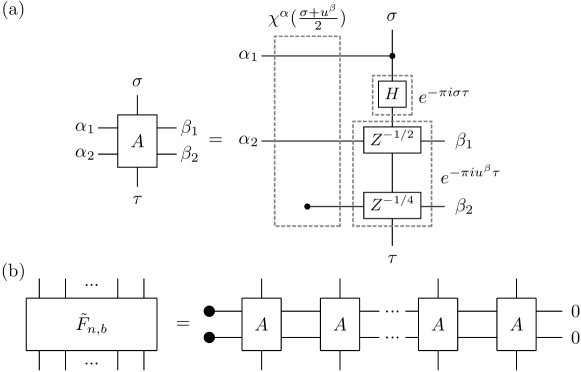
up to the choice of convention for normalization and complex conjugation. Relative to the formula (2.2) for the QFT/DFT, in the AQFT we discard all terms in the exponent with . If we recover the exact QFT, and if we get the Hadamard transform. The quantum circuits for the QFT and AQFT are shown in Fig. 6.2. We prove the following theorem regarding the connection to interpolative decomposition:

Theorem 5.
The -qubit AQFT with approximation level can be expressed exactly as a rank- MPO in which all of the internal cores are given by
| (6.2) |
where for , and are the indicator functions
The leftmost core is given by , and the rightmost core is given by .
Proof.
We adopt the notation for arbitrary bit strings of arbitrary length. Intuitively the notation indicates a binary decimal expansion. With this notation, for any we can express the -qubit AQFT with approximation level as
Indeed, for each , note that in (6.1) all the terms with contribute only integer multiples of in the exponent, which all vanish.
Now for any , we can uniquely write and for bit strings and . We will identify and with these respective bit strings in the notation.
Then define
and
| (6.3) | ||||
Note that , and thus by setting we recover the AQFT, i.e. .
Our goal is to prove that
| (6.4) |
or in the shorthand of the preceding sections, in which the left-hand side indicates the result of attaching the core to the right of . Direct computation reveals that , which precisely matches the leftmost core from the statement of the theorem. Thus the claim (6.4) will complete the proof of the theorem. We now turn to the proof of this claim.
In fact we can derive the MPO core from the tensor diagram of the AQFT, by directly contracting local tensors in the AQFT circuit. This construction is shown in Fig. 6.2 in the case .
The entrywise error of this MPO relative to the true DFT/QFT can be bounded directly by the exact expression (6.1) for entries, without relying on interpolation error bounds, as follows.
For any two phases separated by an angular distance , we always have
Then for any fixed , the angular distance between the phases of the AQFT entry and the corresponding QFT entry is bounded as . We can compute
Therefore the entrywise error of the -qubit AQFT with approximation level is bounded by .
We see that for a fixed number of qubits, the error of the AQFT decays as where is the bond dimension, and to maintain fixed error tolerance the bond dimension must scale linearly with . On the other hand, in the Chebyshev-Lobatto construction of the QFT MPO, the error decays super-exponentially with the bond dimension for a fixed number of qubits. Meanwhile, to maintain fixed error, the bond dimension need only scale sublinearly with . Thus the piecewise constant interpolation used implicitly by the AQFT yields a less efficient MPO approximation for the QFT. On the other hand, the AQFT is presented quite naturally as a quantum circuit. Whether other interpolative constructions can yield more efficient quantum circuits that approximate the QFT is an interesting open question.
References
- [1] Jielun Chen, E.M. Stoudenmire and Steven R. White “Quantum Fourier Transform Has Small Entanglement” In PRX Quantum 4 American Physical Society, 2023, pp. 040318 DOI: 10.1103/PRXQuantum.4.040318
- [2] P.W. Shor “Algorithms for quantum computation: discrete logarithms and factoring” In Proceedings 35th Annual Symposium on Foundations of Computer Science, 1994, pp. 124–134 DOI: 10.1109/SFCS.1994.365700
- [3] M. Fannes, B. Nachtergaele and R.. Werner “Finitely correlated states on quantum spin chains” In Communications in Mathematical Physics 144.3, 1992, pp. 443–490 DOI: 10.1007/BF02099178
- [4] A. Klümper, A. Schadschneider and J. Zittartz “Groundstate properties of a generalized VBS-model” In Zeitschrift für Physik B Condensed Matter 87.3, 1992, pp. 281–287 DOI: 10.1007/BF01309281
- [5] Stellan Östlund and Stefan Rommer “Thermodynamic Limit of Density Matrix Renormalization” In Phys. Rev. Lett. 75 American Physical Society, 1995, pp. 3537–3540 DOI: 10.1103/PhysRevLett.75.3537
- [6] Guifré Vidal “Efficient Classical Simulation of Slightly Entangled Quantum Computations” In Phys. Rev. Lett. 91 American Physical Society, 2003, pp. 147902 DOI: 10.1103/PhysRevLett.91.147902
- [7] B Pirvu, V Murg, J I Cirac and F Verstraete “Matrix product operator representations” In New Journal of Physics 12.2 IOP Publishing, 2010, pp. 025012 DOI: 10.1088/1367-2630/12/2/025012
- [8] Ivan V Oseledets “Tensor-train decomposition” In SIAM Journal on Scientific Computing 33.5 SIAM, 2011, pp. 2295–2317
- [9] Boris Khoromskij “O ( d log N )-Quantics Approximation of N - d Tensors in High-Dimensional Numerical Modeling” In Constructive Approximation - CONSTR APPROX 34, 2009 DOI: 10.1007/s00365-011-9131-1
- [10] D. Coppersmith “An approximate Fourier transform useful in quantum factoring”, 2002 arXiv:quant-ph/0201067 [quant-ph]
- [11] Dorit Aharonov, Zeph Landau and Johann Makowsky “The quantum FFT can be classically simulated”, 2007 arXiv:quant-ph/0611156 [quant-ph]
- [12] Daniel E Browne “Efficient classical simulation of the quantum Fourier transform” In New Journal of Physics 9.5, 2007, pp. 146 DOI: 10.1088/1367-2630/9/5/146
- [13] Nadav Yoran and Anthony J. Short “Efficient classical simulation of the approximate quantum Fourier transform” In Physical Review A 76.4 American Physical Society (APS), 2007 DOI: 10.1103/physreva.76.042321
- [14] Hiroshi Shinaoka et al. “Multiscale Space-Time Ansatz for Correlation Functions of Quantum Systems Based on Quantics Tensor Trains” In Phys. Rev. X 13 American Physical Society, 2023, pp. 021015 DOI: 10.1103/PhysRevX.13.021015
- [15] Sergey Dolgov, Boris Khoromskij and Dmitry Savostyanov “Superfast Fourier Transform Using QTT Approximation” In Journal of Fourier Analysis and Applications 18.5, 2012, pp. 915–953
- [16] Kieran J. Woolfe, Charles D. Hill and Lloyd C.. Hollenberg “Scale invariance and efficient classical simulation of the quantum Fourier transform”, 2014 arXiv:1406.0931 [quant-ph]
- [17] Sergey Dolgov and Dmitry Savostyanov “Parallel cross interpolation for high-precision calculation of high-dimensional integrals” In Computer Physics Communications 246, 2020, pp. 106869 DOI: https://doi.org/10.1016/j.cpc.2019.106869
- [18] Dmitry V. Savostyanov “Quasioptimality of maximum-volume cross interpolation of tensors” In Linear Algebra and its Applications 458, 2014, pp. 217–244 DOI: https://doi.org/10.1016/j.laa.2014.06.006
- [19] Michael Lindsey “Multiscale interpolative construction of quantized tensor trains”, 2023 arXiv:2311.12554 [math.NA]
- [20] Boris N. Khoromskij “Tensor Numerical Methods for High-dimensional PDEs: Basic Theory and Initial Applications”, 2014 arXiv:1408.4053 [math.NA]
- [21] Nikita Gourianov et al. “A quantum-inspired approach to exploit turbulence structures” In Nature Computational Science 2.1 Springer ScienceBusiness Media LLC, 2022, pp. 30–37 DOI: 10.1038/s43588-021-00181-1
- [22] Erika Ye and Nuno F.. Loureiro “Quantum-inspired method for solving the Vlasov-Poisson equations” In Phys. Rev. E 106 American Physical Society, 2022, pp. 035208 DOI: 10.1103/PhysRevE.106.035208
- [23] Martin Kiffner and Dieter Jaksch “Tensor network reduced order models for wall-bounded flows”, 2023 arXiv:2303.03010 [physics.flu-dyn]
- [24] A J Daley, C Kollath, U SchollwÃPck and G Vidal “Time-dependent density-matrix renormalization-group using adaptive effective Hilbert spaces” In Journal of Statistical Mechanics: Theory and Experiment 2004.04, 2004, pp. P04005 DOI: 10.1088/1742-5468/2004/04/P04005
- [25] Steven R. White and Adrian E. Feiguin “Real-Time Evolution Using the Density Matrix Renormalization Group” In Phys. Rev. Lett. 93 American Physical Society, 2004, pp. 076401 DOI: 10.1103/PhysRevLett.93.076401
- [26] G. Vidal “Classical Simulation of Infinite-Size Quantum Lattice Systems in One Spatial Dimension” In Phys. Rev. Lett. 98 American Physical Society, 2007, pp. 070201 DOI: 10.1103/PhysRevLett.98.070201
- [27] Yingzhou Li et al. “Butterfly Factorization” In Multiscale Modeling & Simulation 13.2, 2015, pp. 714–732 DOI: 10.1137/15M1007173
- [28] John P Boyd “A fast algorithm for Chebyshev, Fourier, and sinc interpolation onto an irregular grid” In Journal of Computational Physics 103.2, 1992, pp. 243–257 DOI: https://doi.org/10.1016/0021-9991(92)90399-J
- [29] Lloyd N. Trefethen “Approximation Theory and Approximation Practice, Extended Edition” Philadelphia, PA, USA: SIAM-Society for IndustrialApplied Mathematics, 2019
- [30] Alan Edelman, Peter McCorquodale and Sivan Toledo “The Future Fast Fourier Transform?” In SIAM J. Sci. Comput. 20, 1997, pp. 1094–1114 URL: https://api.semanticscholar.org/CorpusID:1837696