[1,2]Tyler J. Hague
1]\orgnameNorth Carolina A&T State University, \orgaddress\cityGreensboro, \stateNorth Carolina \postcode27411, \countryUSA 2] \orgnameLawrence Berkeley National Laboratory, \orgaddress\cityBerkeley, \stateCalifornia \postcode94720, \countryUSA 3] \orgnameThomas Jefferson National Accelerator Facility, \orgaddress\cityNewport News, \stateVirginia \postcode23606, \countryUSA 4]\orgnameThe Governor’s School for Science and Technology, \orgaddress\cityHampton, \stateVirginia \postcode23666, \countryUSA
Direct Comparison of using a -Transformation instead of the traditional for Extraction of the Proton Radius from Scattering Data
Abstract
A discrepancy in the determination of the proton’s charge radius, , between muonic hydrogen spectroscopy versus classic atomic spectroscopy and electron scattering data has become known as the proton radius puzzle. Extractions of from electron scattering data require determination of the slope of the proton’s charge form factor, , in the limit of through fitting and extrapolation. Some works have presented the -transformation fitting technique as the best choice for this type of extraction due to the true functional form of being mathematically guaranteed to exist within the parameter-space of the fit function. In this work, we test this claim by examining the mathematical bias and variances introduced by this technique as compared to the more traditional fits using statistically sampled parameterizations with known input radii. Our tests conclude that the quality of the -transformation technique depends on the range of data used. In the case of new experiments, the fit function and technique should be selected in advance by generating realistic pseudodata and assessing the power of different techniques.
1 Motivation
The Proton Radius Puzzle and the recent increase in available elastic electron-proton scattering data has invigorated discussions into the best methodology for analyzing elastic scattering data to extract the proton electric form factor, [1]. The Proton Radius Puzzle refers to a disagreement in the proton rms charge radius, (written as henceforth), when measured with a new muonic hydrogen spectroscopy technique versus conventional measurement techniques (atomic hydrogen spectroscopy and scattering).
Of particular note is the discussion surrounding the technique for extracting from scattering data, as it often requires one to make model-dependent analysis choices that affect the final result [2]. In the case where a theoretical model, such as in Ref. [3], is not used, the most impactful choice is that of the fit function and any constraints on that function.
As has been shown [4, 5] that the consistent definition of the proton’s charge radius for all types of radius measurements is
| (1) |
and thus simply determined by the slope of at a . For electron scattering, which cannot be measured to , the implication of this is that must be fit with some functional form and then extrapolated to to determine the slope as it approaches the limit. This has proven to be a challenge, as the true functional form of is not known. As such, the form chosen must be sufficiently flexible so as to contain the true value of within its parameter-space as well as robust enough to not diverge rapidly outside of the region of fitted data, particularly as .
One such method that has seen increased use is the so-called -transformation [6]. In this scheme, the negative four-momentum transfer, , range is conformally mapped to a unit circle. This mapping is done with the formalism:
| (2) |
where , is the highest mapped value, and is a free parameter.
The use of the -transformation is well-motivated. This method is the standard tool for meson transition form factor studies [6, 7, 8, 9, 10, 11, 12]. By applying this mapping with a cut below the two-pion production threshold, the form factor is restricted to the region of analyticity (i.e. it can be represented by a convergent power series). This implies that with a sufficient number of parameters the uncertainty from truncating a power series fit can be minimized, while still arriving at a function with sufficient predictive power. In all, it is an enticing choice that has been used in a large number of analyses [13, 14, 15, 16, 17].
When fitting -transformed data, Eq. 1 must be adjusted to accommodate this coordinate transform:
| (3) |
However, this method is not without it’s drawbacks [18]. Namely, by nature of design, while the true form factor exists within this parameter-space, so do many incorrect form factor parameterizations that can create local minima in the fitting routine. One posited solution to this is the use of physically motivated constraints on the power series coefficients (Ref. [6] suggests using as the coefficients for a -th order power series). The use of these constraints, while conservative, introduces a model-dependence to the fit. Model-dependence, in and of itself, is not problematic; constraints placed on typical form factor polynomial fit (or any other commonly used functions) are model assumptions on the shape and behavior of the form factor. This is only to say that one must take care and be aware of the ramifications of model inputs.
Studies similar to this one have been performed previously, as in Refs. [19, 20], which we have used as a framework for our study. Particularly, we aim to address claims made in Ref. [21] that reanalyzes the PRad [22] proton electric form factor data using the -transformation technique. A claim is made that the PRad proton radius uncertainties are underestimated due to the use of the “Rational(1,1)” fit function instead of the -transformation technique. This claim, if justified, naturally leads to a conclusion that the results from the -transformation technique are a lower limit on precision and accuracy in the extraction of the proton radius when using realistic data. This work aims to test that claim.
Here, we aim study the power of this technique to accurately measure the proton charge radius relative to that of other techniques. We acknowledge that the Ref. [6] posit that trial fits of model data are problematic, as models have to make assumptions on the behavior of the form factor. However, we argue that by studying the technique with several models the affects of these assumptions can be mitigated and a better understanding of the technique can be realized.
2 Method
In this study we closely follow the methodology of Ref. [19]. To test the robustness of the -transformation, we generate pseudodata from parameterizations with a known radius. These pseudodata are then analyzed with several fit functions both in and transformed to . This technique allow us to assess the sensitivity of the conformal mapping to the input and statistical fluctuations of data. For this study, we use 6 different parameterizations of as generators:
-
•
Alarcón, Higinbotham, Weiss, and Ye (AW) fit [3], a parameterization in terms of radius-independent and -dependent parts (fm)
-
•
Arrington, Melnitchouk, and Tjon (AMT) fit [23], a rational(3,5) parameterization (fm)
-
•
Arrington fit [24], an inverse-polynomial fit (fm)
- •
-
•
Standard dipole fit [28] (fm)
-
•
Kelly fit [29], a rational(1,3) fit (fm)
Each of these parameterizations are used to generate equally spaced (in ) values of and apply an uncertainty of to each point, corresponding to a uncertainty on the measured cross section. These pseudodata begin at GeV2 and are spaced every GeV2 up to a variable cutoff . is varied by adding a single data point at a time up to a total of 500 points (that is, to GeV2). At each value, 5000 data sets are generated for each parameterization where each data point is smeared by a Gaussian distribution with a standard deviation equal to the uncertainty on the point.
A keen eye may note that some of these parameterizations incorporate corrections for two-photon exchange (TPE), while others do not. We make no attempt to change this as, particularly at high , the corrections for TPE are quite small often at the sub-percent level [30]. While TPE has been suggested as a contribution to the Proton Radius and Proton Form Factor Puzzles, there is no clear consensus as to whether it can account for these differences [31]. While the inclusion or exclusion of TPE will change the underlying form of the data, our work here assumes no knowledge of the underlying form and is testing different fit functions ability to extrapolate the slope to without this knowledge. We do not need the fit function to explain any other physical quantities or to be a true representation of the underlying function of the form factor.
Each data set is fit with polynomials of increasing order, , as defined by
| (4) |
where is a normalization term. By examining Eqs. 1 and 4, the radius is then extracted as . We also explore applying bounds to the fitting parameters and the use of Rational(N,M)-type functions as used in the recent PRad analysis [22]. For each of the 5000 fits done with each polynomial at each point, the extracted radius, , and are recorded. The final radius from each polynomial at each point is treated to be the radius extracted from the mean slope of all fits and the uncertainty of the slope is taken to be the standard deviation of the slopes fitted and then propagated to the mean extracted radius. Additionally, to assess the power of the fitting techniques, at each point we calculate the Mean Squared Error as
| (5) |
where bias is the difference between the mean extracted radius and the input radius, and is the rms-spread of extracted radii.
Each of these data sets is then transformed from to using Eq. 2. For this work, we set , where is the charged pion mass, to restrict data below the two-pion production threshold and . These values were chosen to match the values that were used in the proof-of-concept performed in Ref. [6]. The -transformed data is then fit with polynomials of increasing order, (analogous to Eq. 4 with replaced by ). This functional form, along with this choice of , allows us to write Eq. 3 as .
These and -transformed data are then refit with a polynomial but with added bounds to constrain the fits. In each of these, prescribed bounds from literature are followed for the [2] and [6] data. As the -transformation dramatically changes the shape of the data so that bounds for data in are not applicable to -transformed data and vice versa. This means that the bounds applied to fits in and fits in are not equivalent to each other. However, given that the techniques allow for different formulation of bounds on the fit parameters, the authors assert that the most fair technique to compare (un)bounded fits in to (un)bounded fits in .
When assessing the quality of these fits in this study, there are two qualities to keep in mind:
-
1.
How well does the fit reflect the data?
-
2.
How well does the fit extract the input radius?
The first question is easily addressed with a simple ‘goodness of fit’ test. In this work, we report the mean and standard deviation of the reduced chi-squared, , calculated for each fit at each . A of approximately 1 indicates that the fit represents the data well, whereas indicates underfitting and indicates overfitting. An important note is that while a satisfactory value is critical for extracting the proton radius, as the data must be properly fit, it does not indicate that the fit will accurately extrapolate to guarantee a correct radius extraction [32]. This statement is even more pertinent as additional terms are added to the fit. Additional terms bring in additional moments that can cause the fit function to vary wildly and unpredictably when extended beyond the range of the measured (or simulated in this case) data.
The second question is addressed by studying the bias and the variance of the extracted radii. The bias is defined as the difference of the mean radius extraction at each and the input model radius. The variance is the standard deviation of the mean extracted radius. In this context, both of these quantities are best assessed when compared to the magnitude of the proton radius puzzle; an unreasonably large bias could yield a result that suggests the incorrect solution to the puzzle, whereas an unreasonably large variance would be unable to discern between the purported solutions. To aid in this assessment, lines representing the magnitude of the proton radius puzzle are added to the bias-variance plots in this work. As these two values can often be inversely correlated when optimizing a fit, we choose to define the error using the Mean Squared Error as in Eq. 5. A smaller MSE indicates an overall improvement in the radius extraction. It should be noted that just as having does not indicate that the extracted radius will be correct, having a low MSE is also insufficient if the fit does not well represent the data. The two properties must be taken together to show that the fit can both reproduce the data and extract the correct radius.
All figures in this article show the fitting techniques applied to the AMT parameterization as an illustrative set. See the Supplemental Information for this work for the full set of figures for all parameterizations as well as textual descriptions of all figures.
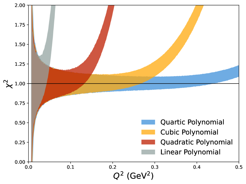
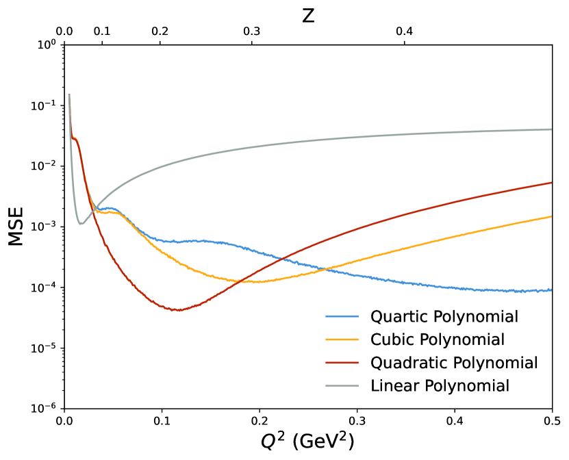
3 Results with unbounded polynomials
The first test we perform on using this methodology is with unbounded polynomials. The authors note that while Ref. [6] proposes that bounds of be used, these bounds, while conservative, are based on a vector-dominance model. In order to initially assess the robustness in the least model-dependent way, we opt to start by omitting any bounds.
Comparing the outputs of the unbounded polynomial fits in Figs. 1 and 2, we can see that there is a trade-off between choosing to fit in or . The unbounded fit has a larger mean bias, that decreases with increasing polynomial order. However, this fit has very little variance in the fit value once a moderate cutoff is reached. The unbounded fit, on the other hand, has a much smaller mean bias for most models checked (though for some models it diverges rapidly once past a moderate cutoff). The trade-off is that the variance in results from the fit is quite large.
Given these results, it is ill-advised to use either of these methods blindly. There may exist some data set where one of these is the optimal choice; however that data set does not exist within this exercise. When comparing the fits in to the choice is, in essence, between a highly repeatable incorrect answer or a potentially correct answer that is not repeatable.


4 Results from bounded polynomial fits
The next test involves placing bounds on the fit parameters. As discussed in the previous section, Ref. [6] proposes that, for the fit of -transformed data, bounds of be used. The bounds are determined by beginning with a model-independent dispersion relation analysis, but then applies a model-dependent vector-dominance ansatz. The calculations could prescribe a more rigid set of bounds than this, however Ref. [6] decided that it was most appropriate to suggest a conservative implementation to minimize the model dependence.
For the fit we follow the prescription of Ref. [2] and require that the fit parameters alternate signs. This bounded regression forces the result to approximate a monotonic function (in this case, non-increasing). This technique reduces the risk that the fit parameters will have dramatic fluctuations when extrapolated beyond the fit region.
The results of these fits, seen in Figs. 3 and 4, fall largely in line with the results of the unbounded polynomial fits. The main effect is a reduction of the variance, most notably seen below GeV2. In this region, the variance is still too large to effectively resolve the proton radius puzzle. At above this, the difference is negligible. The fit in still has a very large bias and the fit in with the vector-dominance bounds has very large variance.


5 Results from fitting with a Rational(N,M) function
The final functional form used is a Rational(N,M) function. A Rational(N,M) function is defined as the form
| (6) |
with as a normalization factor. As an example, the Rational(1,1) function then parameterizes the data as
| (7) |
where the extracted radius is . This functional form was used for the extraction of the proton radius from the PRad experiment [22]. The decision was made by studying various fitters on generated pseudodata (much like this study) and selecting the most robust fitter for the range of the measurement [20].
In this study, we vary N and M within the range of while restricting them to be within of each other. The results of these fits are seen in Fig. 5. An important note here is that the Rational(1,0) function is simply a linear polynomial which yields identical behavior to the linear fit in Fig. 1. Increasing the orders N and M simultaneously increases the at which the bias is small compared to the proton radius puzzle, the minimum at which the variance is small compared to the proton radius puzzle, and the time taken for the fits to converge. The reason for the increase in the time to convergence is that Rational(N,M) functions cover a very large parameter-space, such that increasing the order introduces additional local minima that slow down the fit. It is noted that it was attempted to include the Rational(2,2) function here, but convergence of the illustrative fits took a prohibitively lengthy amount of time.
For the fits in , the functional form of a Rational(N,M) function (provided both N and M at least 1) is by far the most precise and has the least bias. Unsurprisingly, given the study done for the PRad experiment, the Rational(1,1) function has minimal bias around for nearly all models (though perfect agreement with the PRad study should not be expected as this analysis uses a higher , different point density, and different point-to-point uncertainties).
This functional form, when applied to data, shows by far the most robust fitting of the parameterizations considered. However, as with all of the fitting forms studied, it will not always be the best choice in all scenarios.
6 Conclusion
From these illustrative fits, there are a number of conclusions that can be drawn:
-
•
When comparing fits in and , both unbound and bound, no technique is clearly superior for extracting the proton radius. The technique that yields lower MSE depends not only on the order of polynomial and the range, but also on the parameterization fit.
-
•
In contrast, the Rational(N,M) fitting procedure, when N and M are both at least 1 and a minimum is reached, consistently has an MSE value of nearly an order of magnitude lower than the other fits, with the exception of when fitting the Bernauer parameterization. It should also be noted that the Rational(N,M) fits behave very poorly for low values, even giving unphysical results for higher (N,M) orders. A caveat to the smaller MSE values is that it is partially driven by the substantially smaller variance of the fits as there appear to be fewer local minima in the parameter-space.
-
•
Applying bounds to the fitting procedure decreases the variance of the extracted radius. This is expected behavior, as bounds limit the phase space of possible solutions. However, bounds appear to do very little to improve the extracted bias. While physically motivated bounds (e.g. the slope must be negative to ensure a positive charge radius) are a useful tool, additional bounds may induce a false belief in the accuracy of the extraction.
-
•
As the true functional form of is not known, no single fitting function will be ideal for every possible data set. As such, it is imperative that any analysis that seeks to extract the proton charge radius does their due diligence to determine the best fitting function for their data. Ref. [20] details a procedure for an analysis of the most robust fitter for a given data range. Highlighting the care that must be taken, this reference also found that Rational(N,M) functions were inadequate for particularly low data.
-
•
The true form factor is guaranteed to lie within the phase space of a polynomial fit in -transformed data. This technique aims not only to accurately extract the proton radius, but to gain insight into the true functional form of the proton form factor. This additional insight comes with a trade-off of increased uncertainties on the extracted proton radius. As thoroughly described in Ref. [33], modeling to explain data and modeling to predict data are two different goals that are not always achieved with identical techniques. The -transformation technique aims to achieve a deeper explanation of the data than the other techniques investigated, which in turn can negatively impact its predictive power.
-
•
As discussed in Sec. 2, it must be stressed that or MSE alone cannot be used to assess the extracted radius from a fit. The of a fit is only related to the ability of the fit to reproduce the fitted data. The MSE of a fit is only related to the extracted and input radius, with no regard to data points that were fit. Both values must be taken together to assess the strength of a particular fit.
In our work, there was no single data set where applying a conformal mapping to the range improved the extraction of the proton charge radius. This result should not imply that this is not a useful technique. Rather, the transformation should be considered a useful tool in the physicists toolbox after they have assessed the correct tool for the job such as Ref. [20] finds that a 2nd order polynomial fit in is a robust fit for the PRad data points.
Acknowledgments
This material is based upon work supported by the U.S. Department of Energy, Office of Science, Office of Nuclear Physics under contracts DE-AC05-06OR23177 and DE-AC02-05CH11231. This material is based upon work supported in part by NSF award PHY-1812421.


References
- \bibcommenthead
- Lorcé [2020] Lorcé, C.: Charge Distributions of Moving Nucleons. Phys. Rev. Lett. 125(23), 232002 (2020) https://doi.org/10.1103/PhysRevLett.125.232002 arXiv:2007.05318 [hep-ph]
- Barcus et al. [2020] Barcus, S.K., Higinbotham, D.W., McClellan, R.E.: How Analytic Choices Can Affect the Extraction of Electromagnetic Form Factors from Elastic Electron Scattering Cross Section Data. Phys. Rev. C 102(1), 015205 (2020) https://doi.org/10.1103/PhysRevC.102.015205 arXiv:1902.08185 [physics.data-an]
- Alarcón et al. [2019] Alarcón, J.M., Higinbotham, D.W., Weiss, C., Ye, Z.: Proton charge radius extraction from electron scattering data using dispersively improved chiral effective field theory. Phys. Rev. C 99(4), 044303 (2019) https://doi.org/10.1103/PhysRevC.99.044303 arXiv:1809.06373 [hep-ph]
- Eides et al. [2001] Eides, M.I., Grotch, H., Shelyuto, V.A.: Theory of light hydrogen - like atoms. Phys. Rept. 342, 63–261 (2001) https://doi.org/10.1016/S0370-1573(00)00077-6 arXiv:hep-ph/0002158
- Miller [2019] Miller, G.A.: Defining the proton radius: A unified treatment. Phys. Rev. C 99(3), 035202 (2019) https://doi.org/10.1103/PhysRevC.99.035202 arXiv:1812.02714 [nucl-th]
- Hill and Paz [2010] Hill, R.J., Paz, G.: Model independent extraction of the proton charge radius from electron scattering. Phys. Rev. D 82, 113005 (2010) https://doi.org/10.1103/PhysRevD.82.113005 arXiv:1008.4619 [hep-ph]
- Boyd et al. [1996] Boyd, C.G., Grinstein, B., Lebed, R.F.: Model independent determinations of anti-neutrino form-factors. Nucl. Phys. B 461, 493–511 (1996) https://doi.org/10.1016/0550-3213(95)00653-2 arXiv:hep-ph/9508211
- Arnesen et al. [2005] Arnesen, M.C., Grinstein, B., Rothstein, I.Z., Stewart, I.W.: A Precision model independent determination of from . Phys. Rev. Lett. 95, 071802 (2005) https://doi.org/10.1103/PhysRevLett.95.071802 arXiv:hep-ph/0504209
- Becher and Hill [2006] Becher, T., Hill, R.J.: Comment on form-factor shape and extraction of from . Phys. Lett. B 633, 61–69 (2006) https://doi.org/10.1016/j.physletb.2005.11.063 arXiv:hep-ph/0509090
- Hill [2006a] Hill, R.J.: The Modern description of semileptonic meson form factors. eConf C060409, 027 (2006) arXiv:hep-ph/0606023
- Hill [2006b] Hill, R.J.: Constraints on the form factors for and implications for . Phys. Rev. D 74, 096006 (2006) https://doi.org/10.1103/PhysRevD.74.096006 arXiv:hep-ph/0607108
- Bourrely et al. [2009] Bourrely, C., Caprini, I., Lellouch, L.: Model-independent description of decays and a determination of . Phys. Rev. D 79, 013008 (2009) https://doi.org/10.1103/PhysRevD.82.099902 arXiv:0807.2722 [hep-ph]. [Erratum: Phys.Rev.D 82, 099902 (2010)]
- Paz [2012] Paz, G.: The Charge Radius of the Proton. AIP Conf. Proc. 1441(1), 146–149 (2012) https://doi.org/10.1063/1.3700495 arXiv:1109.5708 [hep-ph]
- Epstein et al. [2014] Epstein, Z., Paz, G., Roy, J.: Model independent extraction of the proton magnetic radius from electron scattering. Phys. Rev. D 90(7), 074027 (2014) https://doi.org/10.1103/PhysRevD.90.074027 arXiv:1407.5683 [hep-ph]
- Lee et al. [2015] Lee, G., Arrington, J.R., Hill, R.J.: Extraction of the proton radius from electron-proton scattering data. Phys. Rev. D 92(1), 013013 (2015) https://doi.org/10.1103/PhysRevD.92.013013 arXiv:1505.01489 [hep-ph]
- Ye et al. [2018] Ye, Z., Arrington, J., Hill, R.J., Lee, G.: Proton and Neutron Electromagnetic Form Factors and Uncertainties. Phys. Lett. B 777, 8–15 (2018) https://doi.org/10.1016/j.physletb.2017.11.023 arXiv:1707.09063 [nucl-ex]
- Sick [2018] Sick, I.: Proton charge radius from electron scattering. Atoms 6(1), 2 (2018) https://doi.org/10.3390/atoms6010002 arXiv:1801.01746 [nucl-ex]
- Bernauer and Distler [2016] Bernauer, J.C., Distler, M.O.: Avoiding common pitfalls and misconceptions in extractions of the proton radius. In: ECT* Workshop on the Proton Radius Puzzle (2016)
- Kraus et al. [2014] Kraus, E., Mesick, K.E., White, A., Gilman, R., Strauch, S.: Polynomial fits and the proton radius puzzle. Phys. Rev. C 90(4), 045206 (2014) https://doi.org/10.1103/PhysRevC.90.045206 arXiv:1405.4735 [nucl-ex]
- Yan et al. [2018] Yan, X., Higinbotham, D.W., Dutta, D., Gao, H., Gasparian, A., Khandaker, M.A., Liyanage, N., Pasyuk, E., Peng, C., Xiong, W.: Robust extraction of the proton charge radius from electron-proton scattering data. Phys. Rev. C 98(2), 025204 (2018) https://doi.org/10.1103/PhysRevC.98.025204 arXiv:1803.01629 [nucl-ex]
- Paz [2021] Paz, G.: Model Independent Extraction of the Proton Charge Radius from PRad data. Mod. Phys. Lett. A 36, 2150143 (2021) https://doi.org/10.1142/S0217732321501431 arXiv:2004.03077 [hep-ph]
- Xiong et al. [2019] Xiong, W., et al.: A small proton charge radius from an electron–proton scattering experiment. Nature 575(7781), 147–150 (2019) https://doi.org/10.1038/s41586-019-1721-2
- Arrington et al. [2007] Arrington, J., Melnitchouk, W., Tjon, J.A.: Global analysis of proton elastic form factor data with two-photon exchange corrections. Phys. Rev. C 76, 035205 (2007) https://doi.org/10.1103/PhysRevC.76.035205 arXiv:0707.1861 [nucl-ex]
- Arrington [2004] Arrington, J.: Implications of the discrepancy between proton form factor measurements. Phys. Rev. C 69, 022201 (2004) https://doi.org/10.1103/PhysRevC.69.022201 arXiv:nucl-ex/0309011
- Bernauer [2010] Bernauer, J.C.: Measurement of the elastic electron-proton cross section and separation of the electric and magnetic form factor in the Q2 range from 0.004 to 1 (GeV/c)2. PhD thesis, Johannes Gutenburg Universität Mainz (2010)
- Bernauer et al. [2010] Bernauer, J.C., et al.: High-precision determination of the electric and magnetic form factors of the proton. Phys. Rev. Lett. 105, 242001 (2010) https://doi.org/10.1103/PhysRevLett.105.242001 arXiv:1007.5076 [nucl-ex]
- Bernauer et al. [2014] Bernauer, J.C., et al.: Electric and magnetic form factors of the proton. Phys. Rev. C 90(1), 015206 (2014) https://doi.org/10.1103/PhysRevC.90.015206 arXiv:1307.6227 [nucl-ex]
- Hand et al. [1963] Hand, L.N., Miller, D.G., Wilson, R.: Electric and Magnetic Formfactor of the Nucleon. Rev. Mod. Phys. 35, 335 (1963) https://doi.org/10.1103/RevModPhys.35.335
- Kelly [2004] Kelly, J.J.: Simple parametrization of nucleon form factors. Phys. Rev. C 70, 068202 (2004) https://doi.org/10.1103/PhysRevC.70.068202
- Arrington [2013] Arrington, J.: Coulomb corrections in the extraction of the proton radius. J. Phys. G 40, 115003 (2013) https://doi.org/10.1088/0954-3899/40/11/115003 arXiv:1210.2677 [nucl-ex]
- Schmidt [2020] Schmidt, A.: How much two-photon exchange is needed to resolve the proton form factor discrepancy? J. Phys. G 47(5), 055109 (2020) https://doi.org/10.1088/1361-6471/ab7ec1 arXiv:1907.07318 [nucl-ex]
- Andrae et al. [2010] Andrae, R., Schulze-Hartung, T., Melchior, P.: Dos and don’ts of reduced chi-squared (2010)
- Shmueli [2010] Shmueli, G.: To Explain or to Predict? Statistical Science 25(3), 289–310 (2010) https://doi.org/%****␣main.bbl␣Line␣550␣****10.1214/10-STS330