Diophantine tuples and multiplicative structure of shifted multiplicative subgroups

A set $\{a_{1},a_{2},\ldots,a_{m}\}$ of distinct positive integers is a Diophantine $m$-tuple if the product of any two distinct elements in the set is one less than a square. The first known example of integral Diophantine $4$-tuples is $\{1,3,8,120\}$ which was studied by Fermat. The Diophantine $4$-tuple was extended by Euler to the rational $5$-tuple $\{1,3,8,120,\frac{777480}{8288641}\}$, and it had been conjectured that there is no Diophantine $5$-tuple. The difficulty of extending Diophantine tuples can be explained by its connection to the problem of finding integral points on elliptic curves: if $\{a,b,c\}$ forms a Diophantine $3$-tuple, in order to find a positive integer $d$ such that $\{a,b,c,d\}$ is a Diophantine $4$-tuple, we need to solve the following simultaneous equation for $d$:

This is related to the problem of finding an integral point $(d,str)$ on the following elliptic curve

From this, we can deduce that there are no infinite Diophantine $m$-tuples by Siegel’s theorem on integral points. On the other hand, Siegel’s theorem is not sufficient to give an upper bound on the size of Diophantine tuples due to its ineffectivity. In the same vein, finding a Diophantine tuple of size greater than or equal to $5$ is related to the problem of finding integral points on hyperelliptic curves of genus $g\geq 2$. Despite the aforementioned difficulties, the conjecture on the non-existence of Diophantine $5$-tuples was recently proved to be true in the sequel of important papers by Dujella [9], and He, Togbé, and Ziegler [22].

The definition of Diophantine $m$-tuples has been generalized and studied in various contexts. We refer to the recent book of Dujella [10] for a thorough list of known results on the topic and their reference. In this paper, we focus on the following generalization of Diophantine tuples: for each $n\geq 1$ and $k\geq 2$, we call a set $\{a_{1},a_{2},\ldots,a_{m}\}$ of distinct positive integers a Diophantine $m$-tuple with property $D_{k}(n)$ if the product of any two distinct elements is $n$ less than a $k$-th power. We write

Similar to the classical case, the problem of finding $M_{k}(n)$ for $k\geq 3$ and $n\geq 1$ is related to the problem of counting the number of integral points of the superelliptic curve

The theorem of Faltings [13] guarantees that the above curve has only finitely many integral points, and this, in turn, implies that a set with property $D_{k}(n)$ must be finite. The known upper bounds for the number of integral points depend on the coefficients of $f(x)$. The Caporaso-Harris-Mazur conjecture [6] implies that $M_{k}(n)$ is uniformly bounded, independent of $n$. For other conditional bounds, we refer the readers to Subsection 2.4.

Unconditionally, in [4], Bugeaud and Dujella showed that $M_{3}(1)\leq 7,M_{4}(1)\leq 5,M_{k}(1)\leq 4$ for $5\leq k\leq 176$, and the uniform bound $M_{k}(1)\leq 3$ for any $k\geq 177$. On the other hand, the best-known upper bound on $M_{2}(n)$ is $(2+o(1))\log n$, due to Yip [39]. Very recently, Dixit, Kim, and Murty [7] studied the size of a generalized Diophantine $m$-tuple with property $D_{k}(n)$, improving the previously best-known upper bound $M_{k}(n)\leq 2|n|^{5}+3$ for $k\geq 5$ given by Bérczes, Dujella, Hajdu and Luca [2] when $n\to\infty$. They showed that if $k$ is fixed and $n\to\infty$, then $M_{k}(n)\ll_{k}\log n$. Following their proof in [7], the bound can be more explicitly expressed as $M_{k}(n)\leq(3\phi(k)+o(1))\log n$ when $k\geq 3$ is fixed, $n\to\infty$, and $\phi$ is the Euler phi function. Note that their upper bound on $M_{k}(n)$ is perhaps not desirable. Indeed, it is natural to expect that $M_{k}(n)$ would decrease if $n$ is fixed, and $k$ increases, since $k$-th powers become sparser. Instead, our new upper bounds on $M_{k}(n)$ support this heuristic.

In this paper, we provide a significant improvement on the upper bound of $M_{k}(n)$ by using a novel combination of Stepanov’s method and Gallagher’s larger sieve inequality. In order to state our first result, we define the following constant

for each $k\geq 2$, where the minimum is taken over all nonempty subsets $\mathcal{I}$ of the set

and $T_{\mathcal{I}}=\sum_{i\in\mathcal{I}}\sqrt{\gcd(i-1,k)}$.

The constant $\eta_{k}$ is essentially computed via the optimal collection of “admissible” residue classes when applying Gallagher’s larger sieve (see Section 5). Note that when $\mathcal{I}=\{1\}$, we have $T_{\mathcal{I}}=\sqrt{k}$, and hence we have $\eta_{k}\leq\frac{1}{k}$. In particular, if $k\geq 3$ is fixed and $n\to\infty$, inequality 1.4 implies the upper bound

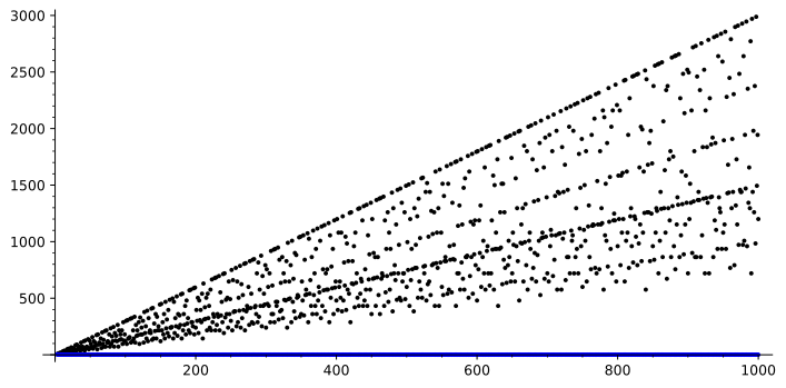
which already improves the best-known upper bound $M_{k}(n)\leq(3\phi(k)+o(1))\log n$ of [7] that we mentioned earlier substantially. In Appendix A, we illustrate the bound in inequality 1.4: for $2\leq k\leq 1001$, we compute the suggested upper bound

of $\gamma_{k}=\limsup_{n\to\infty}\frac{M_{k}(n)}{\log n}$. From Figure A.1, one can compare the bound of $M_{k}(n)$ in Theorem 1.2 with the bound in [7]. From inequality 1.5, we see $\gamma_{k}$ is uniformly bounded by $6$. Table A.2 illustrates better upper bounds on $\gamma_{k}$ for $2\leq k\leq 201$. In particular, we use a simple greedy algorithm to determine $\eta_{k}$ for a fixed $k$. We also refer to Subsection 5.3 for a simple upper bound on $\eta_{k}$, which well approximates $\eta_{k}$ empirically.

At first glance, Theorem 1.2 improves the bound in [7] of $M_{k}(n)$ by only a constant multiplicative factor when $k$ is fixed. Nevertheless, note that Theorem 1.2 holds uniformly for $k$ and $n$ as long as $\log k\leq c^{\prime}\sqrt{\log\log n}$. Thus, when $k$ is assumed to be a function of $n$ which increases as $n$ increases, we can break the “$\log n$ barrier” in [7], that is, $M_{k}(n)=O_{k}(\log n)$, and provide a dramatic improvement.

The proofs of Theorem 1.2 and Theorem 1.3 require the study of (generalized) Diophantine tuples over finite fields, which we discuss below.

A Diophantine $m$-tuple with property $D_{d}(\lambda,\mathbb{F}_{q})$ is a set $\{a_{1},\ldots,a_{m}\}$ of $m$ distinct elements in $\mathbb{F}_{q}^{*}$ such that $a_{i}a_{j}+\lambda$ is a $d$-th power in $\mathbb{F}_{q}^{*}$ or $0$ whenever $i\neq j$. Moreover, we also define the strong Diophantine tuples in finite fields motivated by Dujella and Petričević [11]: a strong Diophantine $m$-tuple with property $SD_{d}(\lambda,\mathbb{F}_{q})$ is a set $\{a_{1},\ldots,a_{m}\}$ of $m$ distinct elements in $\mathbb{F}_{q}^{*}$ such that $a_{i}a_{j}+\lambda$ is a $d$-th power in $\mathbb{F}_{q}^{*}$ or $0$ for any choice of $i$ and $j$. Unlike the natural analog for the classical Diophantine tuples (of property $D_{2}(1)$), it makes sense to talk about the strong Diophantine tuples in $\mathbb{F}_{q}$. The strong generalized Diophantine tuples with property $D_{k}(n)$ in for general $k$ and $n$ are also meaningful to study: the problem of counting the explicit size of the strong generalized Diophantine tuples with property $D_{k}(n)$ involves the problem of counting solutions of the equations appearing in the statement of Pillai’s conjecture. Theorem 1.2 can be improved for strong generalized Diophantine tuples with property $D_{k}(n)$; see Theorem 5.2.

The generalizations of Diophantine tuples over finite fields are of independent interest. Perhaps the most interesting question to explore is the exact analog of estimating $M_{k}(n)$ as discussed in Subsection 1.1. Indeed, estimating the size of the largest Diophantine tuple with property $SD_{d}(\lambda,\mathbb{F}_{q})$ or with property $D_{d}(\lambda,\mathbb{F}_{q})$ is of particular interest for the application of Diophantine tuples (over integers) as discussed in [1, 7, 8, 16, 24]. Similarly, we denote

Note that when $\lambda=0$, it is trivial that $MSD_{d}(\lambda,\mathbb{F}_{q})=MD_{d}(\lambda,\mathbb{F}_{q})=\frac{q-1}{d}$. Thus, we always assume $\lambda\neq 0$ throughout the paper. In Section 3, we give an upper bound $\sqrt{q}+O(1)$ of $MSD_{d}(\lambda,\mathbb{F}_{q})$ and $MD_{d}(\lambda,\mathbb{F}_{q})$. More precisely, we prove the following proposition using a double character sum estimate. We refer to the bounds in the following proposition as the “trivial” upper bound.

For the case $q=p$, similar bounds of Proposition 1.4 are known previously in [1, 7, 17]. On the other hand, Proposition 1.4 gives an almost optimal bound of $MSD_{d}(\lambda,\mathbb{F}_{q})$ and $MD_{d}(\lambda,\mathbb{F}_{q})$ when $q$ is a square (Theorem 1.6). Our next theorem improves the trivial upper bounds in Proposition 1.4 by a multiplicative constant factor $\sqrt{1/d}$ or $\sqrt{2/d}$ when $q=p$ is a prime.

We remark that our new bound on $MSD_{d}(\lambda,\mathbb{F}_{p})$ is sometimes sharp. For example, we get a tight bound for a prime $p\in\{5,7,11,13,17,23,31,37,41,53,59,61,113\}$ when $d=2$ and $\lambda=1$. See also Theorem 4.7 and Remark 4.8 for a generalization of Theorem 1.5 over general finite fields with non-square order under some extra assumptions.

Nevertheless, in the case of finite fields of square order, we improve Proposition 1.4 by a little bit under some minor assumptions; see Theorem 4.5. Surprisingly, this tiny improvement turns out to be sharp for many infinite families of $(q,d,\lambda)$. Equivalently, we determine $MD_{d}(\lambda,{\mathbb{F}}_{q})$ and $MSD_{d}(\lambda,{\mathbb{F}}_{q})$ exactly in those families. In the following theorem, we give a sufficient condition so that $MD_{d}(\lambda,{\mathbb{F}}_{q})$ and $MSD_{d}(\lambda,{\mathbb{F}}_{q})$ can be determined explicitly.

Under the assumptions on Theorem 1.6, $\alpha{\mathbb{F}}_{\sqrt{q}}^{*}$ satisfies the required property $SD_{d}(\lambda,\mathbb{F}_{q})$ and $D_{d}(\lambda,\mathbb{F}_{q})$. Compared to Theorem 1.5, it is tempting to conjecture that such an algebraic construction (which is unique to finite fields with proper prime power order) is the optimal one with the required property. Given Proposition 1.4, to show such construction is optimal, it suffices to rule out the possibility of a Diophantine tuple with property $SD_{d}(\lambda,\mathbb{F}_{q})$ and $D_{d}(\lambda,\mathbb{F}_{q})$ of size $\sqrt{q}$. While this seems easy, it turned out that this requires non-trivial efforts.

Next, we give concrete examples where Theorem 1.6 applies.

One key ingredient of the proof of Theorem 1.5 and Theorem 1.6 is Theorem 1.1. Indeed, Theorem 1.1 can also be viewed as on an upper bound of a bipartite version of Diophantine tuples over finite fields. For the applications to strong Diophantine tuples, Theorem 1.1 is sufficient. On the other hand, to obtain upper bounds on Diophantine tuples (which are not necessarily strong Diophantine tuples), we also need a version of Theorem 1.1 for restricted product sets, which can be found as Theorem 4.2. Indeed, Theorem 1.1 alone only implies a weaker bound of the form $2\sqrt{p/d}$ for $MSD_{d}(\lambda,{\mathbb{F}}_{p})$; see Remark 4.3.

A well-known conjecture of Sárközy [30] asserts that the set of nonzero squares $S_{2}=\{x^{2}:x\in{\mathbb{F}}_{p}^{*}\}\subset{\mathbb{F}}_{p}$ cannot be written as $S_{2}=A+B$, where $A,B\subset{\mathbb{F}}_{p}$ and $|A|,|B|\geq 2$, provided that $p$ is a sufficiently large prime. This conjecture essentially predicts that the set of quadratic residues in a prime field cannot have a rich additive structure. Similarly, one expects that any non-trivial shift of $S_{2}$ cannot have a rich multiplicative structure. Indeed, this can be made precise via another interesting conjecture of Sárközy [31], which we make progress in the current paper.

We note that it is necessary to take out the element $0$ from the shifted subgroup, for otherwise one can always decompose $S_{2}-\lambda$ as $\{0,1\}\cdot(S_{2}-\lambda)$. It appears that this problem concerning multiplicative decompositions is more difficult than the one concerning additive decompositions stated previously, given that it might depend on the parameter $\lambda$. Inspired by 1.8, we formulate the following more general conjecture for any proper multiplicative subgroup. For simplicity, we denote $S_{d}=S_{d}({\mathbb{F}}_{q})=\{x^{d}:x\in{\mathbb{F}}_{q}^{*}\}$ to be the set of $d$-th powers in ${\mathbb{F}}_{q}^{*}$, equivalently, the subgroup of ${\mathbb{F}}_{q}^{*}$ with order $\frac{q-1}{d}$.

1.9 predicts that a shifted multiplicative subgroup of a finite field admits a non-trivial multiplicative decomposition only when it has a small size. We remark that the integer version of 1.9, namely, for each $k\geq 2$, a non-trivial shift of $k$-th powers in integers has no non-trivial multiplicative decomposition, has been proved and strengthened in a series of papers by Hajdu and Sárközy [18, 19, 20]. On the other hand, to the best knowledge of the authors, 1.9 appears to be much harder and no partial progress has been made. For the analog of 1.9 on the additive decomposition of multiplicative subgroups, we refer to recent papers [21, 31, 33, 38] for an extensive discussion on partial progress.

Our main contribution to 1.9 is the following two results. The first one is a corollary of Theorem 1.1.

In particular, Corollary 1.10 confirms 1.9 under the assumption that $q$ is a prime, $\lambda\in S_{d}$, and $|S_{d}|-1$ is a prime. The second result provides a partial answer to 1.9 asymptotically.

In particular, by setting $n=1$ and $d=2$, our result has the following significant implication to Sárközy’s conjecture [31]: for almost all odd primes $p$, the shifted multiplicative subgroup $(S_{2}({\mathbb{F}}_{p})-1)\setminus\{0\}$ has no non-trivial multiplicative decomposition. In other words, if $\lambda=1$, then Sárközy’s conjecture holds for almost all primes $p$; see Theorem 6.1 for a precise statement.

Some partial progress has been made for 1.9 when the multiplicative decomposition is assumed to have special forms [31, 33]. We also make progress in this direction in Subsection 6.2. In particular, in Theorem 6.6, we confirm the ternary version of 1.9 in a strong sense, which generalizes [31, Theorem 2].

Notations. We follow standard notations from analytic number theory. We use $\pi$ and $\theta$ to denote the standard prime-counting functions. We adopt standard asymptotic notations $O,o,\asymp$. We also follow the Vinogradov notation $\ll$: we write $X\ll Y$ if there is an absolute constant $C>0$ so that $|X|\leq CY$.

Throughout the paper, let $p$ be a prime and $q$ a power of $p$. Let ${\mathbb{F}}_{q}$ be the finite field with $q$ elements and let ${\mathbb{F}}_{q}^{*}={\mathbb{F}}_{q}\setminus\{0\}$. We always assume that $d\mid(q-1)$ with $d\geq 2$, and denote $S_{d}({\mathbb{F}}_{q})=\{x^{d}:x\in{\mathbb{F}}_{q}^{*}\}$ to be the subgroup of ${\mathbb{F}}_{q}^{*}$ with order $\frac{q-1}{d}$. If $q$ is assumed to be fixed, for brevity, we simply write $S_{d}$ instead of $S_{d}({\mathbb{F}}_{q})$.

We also need some notations for arithmetic operations among sets. Given two sets $A$ and $B$, we write the product set $AB=\{ab:a\in A,b\in B\}$, and the sumset $A+B=\{a+b:a\in A,b\in B\}$. Given the definition of Diophantine tuples, it is also useful to define the restricted product set of $A$, that is, $A\hat{\times}A=\{ab:a,b\in A,a\neq b\}$.

Structure of the paper. In Section 2, we introduce more background. In Section 3, using Gauss sums and Weil’s bound, we give an upper bound on the size of the set which satisfies various multiplicative properties based on character sum estimates. In particular, we prove Proposition 1.4. In Section 4, we first prove Theorem 1.1 using Stepanov’s method. At the end of the section, we deduce applications of Theorem 1.1 to Diophantine tuples and prove Theorem 1.5 and Theorem 1.6. Via Gallagher’s larger sieve inequality and other tools from analytic number theory, in Section 5, we prove Theorem 1.2 and Theorem 1.3. In Section 6, we study multiplicative decompositions and prove Theorem 1.11.

We first describe Stepanov’s method [35]. If we can construct a low degree non-zero auxiliary polynomial that vanishes on each element of a set $A$ with high multiplicity, then we can give an upper bound on $|A|$ based on the degree of the polynomial. It turns out that the most challenging part of our proofs is to show that the auxiliary polynomial constructed is not identically zero.

To check that each root has a high multiplicity, standard derivatives might not work since we are working in a field with characteristic $p$. To resolve this issue, we need the following notation of derivatives, known as the Hasse derivatives or hyper-derivatives; see [26, Section 6.4].

Following the definition, we have $E^{(0)}f=f$. We also need the next three lemmas.

In this subsection, we introduce Gallagher’s larger sieve inequality and provide necessary estimations from it. Gallagher’s larger sieve inequality will be one of the main ingredients for the proof of Theorem 1.2. In 1971, Gallagher [15] discovered the following sieve inequality.

As a preparation to apply Gallagher’s larger sieve in our proof, we need to establish a few estimates related to primes in arithmetic progressions. For $(a,k)=1$, we follow the standard notation

For our purposes, $\log k$ could be as large as $\sqrt{\log\log x}$ (for example, see Theorem 1.2), and we need the Siegel-Walfisz theorem to estimate $\theta(x;k,a)$.

A standard application of partial summation with Lemma 2.6 leads to the following corollary.

We also need the following lemma.

Following [7], for each real number $L>0$, we write

It is shown in [7] that $M_{k}(n,3)\ll_{k}1$ as $n\to\infty$. For our application, we show a stronger result that $M_{k}(n,\frac{k}{k-2})\ll_{k}1$ and we will make this estimate explicit and effective. We follow the proof in [7] closely and prove the following proposition, which will be used later in the proof of Theorem 1.2.

Let $k\geq 3$. Let $m=M_{k}(n,\frac{k}{k-2})$ and $A=\{a_{1},a_{2},\ldots,a_{m}\}$ be a generalized $m$-tuple with property $D_{k}(n)$ and $n^{\frac{k}{k-2}}<a_{1}<a_{2}<\cdots<a_{m}$. Consider the system of equations

Clearly, for each $i\geq 3$, $x=a_{i}$ is a solution to this system, and we denote $u_{i},v_{i}$ so that $a_{1}a_{i}+n=u_{i}^{k}$ and $a_{2}a_{i}+n=v_{i}^{k}$. Let $\alpha:=(a_{1}/a_{2})^{1/k}$.

The following lemma is a generalization of [7, Lemma 3.1], showing that $u_{i}/v_{i}$ provides a “good” rational approximation to $\alpha$ if $n$ is large. Note that in [7, Lemma 3.1], it was further assumed that $k$ is odd and $L=3$. Nevertheless, an almost identical proof works, and we skip the proof.

Now we are ready to prove Proposition 2.9. Recall we have the inequality $\sin x\geq\frac{2x}{\pi}$ for $x\in[0,\frac{\pi}{2}]$, and the inequality $s!\geq(s/e)^{s}$ for all positive integers $s$. It follows that

when $k$ is odd, and

when $k$ is even. Thus, when $k\geq 3$, we always have

Therefore, when $n>(2ke)^{k^{2}}$, we can apply Lemma 2.10. Note that the absolute height of $\alpha$ is $H(\alpha)\leq a_{2}^{1/k}$. Since $k\geq 3$, for $14\leq i\leq m$, Lemma 2.10 implies that

moreover, $\max(u_{i},v_{i})=v_{i}>a_{2}^{1/k}\geq\max(H(\alpha),2)$. Therefore, we can apply the quantitative Roth’s theorem due to Evertse [12] (see also [7, Theorem 2.2]) to conclude that

where the implicit constant is absolute.

The Paley graph conjecture on double character sums implies many results of the present paper related to the estimation of character sums. We record the statement of the conjecture (see for example [7, 16]).

The connection between the Paley graph conjecture and the problem of bounding the size of Diophantine tuples was first observed by Güloğlu and Murty in [16]. Let $d\geq 2$ be fixed, $\lambda\in{\mathbb{F}}_{p}^{*}$, where $p\equiv 1\pmod{d}$ is a prime. The Paley graph conjecture trivially implies $MD_{d}(\lambda,{\mathbb{F}}_{p})=p^{o(1)}$ and $MSD_{d}(\lambda,{\mathbb{F}}_{p})=p^{o(1)}$ as $p\to\infty$. Also, the bound on $M_{k}(n)$ in Theorem 1.2 can be improved to $(\log n)^{o(1)}$ (see [7], [16]) when $k$ is fixed and $n\to\infty$. Furthermore, the Paley graph conjecture also immediately implies Sárközy’s conjecture (1.8) in view of Proposition 3.4. However, the Paley graph conjecture itself remains widely open, and our results are unconditional. We refer to [32] and the references therein for recent progress on the Paley graph conjecture assuming $A,B$ have small doubling.

References

- [1] R. Becker and M. R. Murty. Diophantine -tuples with the property . Glas. Mat. Ser. III, 54(74)(1):65–75, 2019.
- [2] A. Bérczes, A. Dujella, L. Hajdu, and F. Luca. On the size of sets whose elements have perfect power -shifted products. Publ. Math. Debrecen, 79(3-4):325–339, 2011.
- [3] S. R. Blackburn, S. V. Konyagin, and I. E. Shparlinski. Counting additive decompositions of quadratic residues in finite fields. Funct. Approx. Comment. Math., 52(2):223–227, 2015.
- [4] Y. Bugeaud and A. Dujella. On a problem of Diophantus for higher powers. Math. Proc. Cambridge Philos. Soc., 135(1):1–10, 2003.
- [5] J. P. Buhler, H. W. Lenstra, Jr., and C. Pomerance. Factoring integers with the number field sieve. In The development of the number field sieve, volume 1554 of Lecture Notes in Math., pages 50–94. Springer, Berlin, 1993.
- [6] L. Caporaso, J. Harris, and B. Mazur. Uniformity of rational points. J. Amer. Math. Soc., 10(1):1–35, 1997.
- [7] A. B. Dixit, S. Kim, and M. R. Murty. Generalized Diophantine -tuples. Proc. Amer. Math. Soc., 150(4):1455–1465, 2022.
- [8] A. Dujella. On the size of Diophantine -tuples. Math. Proc. Cambridge Philos. Soc., 132(1):23–33, 2002.
- [9] A. Dujella. There are only finitely many Diophantine quintuples. J. Reine Angew. Math., 566:183–214, 2004.
- [10] A. Dujella. Diophantine -tuples and Elliptic Curves, volume 79 of Developments in Mathematics. Springer, Cham, 2024.
- [11] A. Dujella and V. Petričević. Strong Diophantine triples. Experiment. Math., 17(1):83–89, 2008.
- [12] J.-H. Evertse. On the quantitative subspace theorem. Zap. Nauchn. Sem. S.-Peterburg. Otdel. Mat. Inst. Steklov. (POMI), 377(Issledovaniya po Teorii Chisel. 10):217–240, 245, 2010.
- [13] G. Faltings. Endlichkeitssätze für abelsche Varietäten über Zahlkörpern. Invent. Math., 73(3):349–366, 1983.
- [14] K. Ford. The distribution of integers with a divisor in a given interval. Ann. of Math. (2), 168(2):367–433, 2008.
- [15] P. X. Gallagher. A larger sieve. Acta Arith., 18:77–81, 1971.
- [16] A. M. Güloğlu and M. R. Murty. The Paley graph conjecture and Diophantine -tuples. J. Combin. Theory Ser. A, 170:105155, 9, 2020.
- [17] K. Gyarmati. On a problem of Diophantus. Acta Arith., 97(1):53–65, 2001.
- [18] L. Hajdu and A. Sárközy. On multiplicative decompositions of polynomial sequences, I. Acta Arith., 184(2):139–150, 2018.
- [19] L. Hajdu and A. Sárközy. On multiplicative decompositions of polynomial sequences, II. Acta Arith., 186(2):191–200, 2018.
- [20] L. Hajdu and A. Sárközy. On multiplicative decompositions of polynomial sequences, III. Acta Arith., 193(2):193–216, 2020.
- [21] B. Hanson and G. Petridis. Refined estimates concerning sumsets contained in the roots of unity. Proc. Lond. Math. Soc. (3), 122(3):353–358, 2021.
- [22] B. He, A. Togbé, and V. Ziegler. There is no Diophantine quintuple. Trans. Amer. Math. Soc., 371(9):6665–6709, 2019.
- [23] A. A. Karatsuba. Distribution of values of Dirichlet characters on additive sequences. Dokl. Akad. Nauk SSSR, 319(3):543–545, 1991.
- [24] S. Kim, C. H. Yip, and S. Yoo. Explicit constructions of Diophantine tuples over finite fields. Ramanujan J., 65(1):163–172, 2024.
- [25] E. Kummer. Über die ergänzungssätze zu den allgemeinen reciprocitätsgesetzen. Journal für die reine und angewandte Mathematik, 44:93–146, 1852.
- [26] R. Lidl and H. Niederreiter. Finite fields, volume 20 of Encyclopedia of Mathematics and its Applications. Cambridge University Press, Cambridge, second edition, 1997.
- [27] S. Macourt, I. D. Shkredov, and I. E. Shparlinski. Multiplicative energy of shifted subgroups and bounds on exponential sums with trinomials in finite fields. Canad. J. Math., 70(6):1319–1338, 2018.
- [28] H. L. Montgomery and R. C. Vaughan. Multiplicative number theory. I. Classical theory, volume 97 of Cambridge Studies in Advanced Mathematics. Cambridge University Press, Cambridge, 2007.
- [29] I. Z. Ruzsa. Cardinality questions about sumsets. In Additive combinatorics, volume 43 of CRM Proc. Lecture Notes, pages 195–205. Amer. Math. Soc., Providence, RI, 2007.
- [30] A. Sárközy. On additive decompositions of the set of quadratic residues modulo . Acta Arith., 155(1):41–51, 2012.
- [31] A. Sárközy. On multiplicative decompositions of the set of the shifted quadratic residues modulo . In Number theory, analysis, and combinatorics, De Gruyter Proc. Math., pages 295–307. De Gruyter, Berlin, 2014.
- [32] T. Schoen and I. D. Shkredov. Character sums estimates and an application to a problem of Balog. Indiana Univ. Math. J., 71(3):953–964, 2022.
- [33] I. D. Shkredov. Any small multiplicative subgroup is not a sumset. Finite Fields Appl., 63:101645, 15, 2020.
- [34] I. E. Shparlinski. Additive decompositions of subgroups of finite fields. SIAM J. Discrete Math., 27(4):1870–1879, 2013.
- [35] S. A. Stepanov. On the number of points of a hyperelliptic curve over a finite prime field. Izv. Akad. Nauk SSSR, Ser. Mat., 33:1171–1181, 1969.
- [36] I. M. Vinogradov. Elements of number theory. Dover Publications, Inc., New York, 1954. Translated by S. Kravetz.
- [37] I. V. Vyugin and I. D. Shkredov. On additive shifts of multiplicative subgroups. Mat. Sb., 203(6):81–100, 2012.
- [38] C. H. Yip. Additive decompositions of large multiplicative subgroups in finite fields. Acta Arith., 213(2):97–116, 2024.
- [39] C. H. Yip. Improved upper bounds on Diophantine tuples with the property . 2024. arXiv:2406.00840. Bull. Aust. Math. Soc., to appear.
Appendix A Algorithm and Computations
We continue our discussion from the introduction on the following constant
It is implicit in [7] that . We also write
Our main result, Theorem 1.2, implies that . In particular, in view of Remark 5.1, it follows that for all and when . In Figure A.1, we pictorially compare our new bound with the bound when .
Recall that for , we defined the constant where the minimum is taken over all nonempty subsets of and
To compute , we use the following simple greedy algorithm with running time . The observation is as follows. If is fixed, our goal is to minimize . Thus, we should choose those residue classes with as large as possible to maximize . Then, we can sort these gcds in decreasing order, and when is fixed, we pick those residue classes corresponding to the largest gcds. The following is a precise description of the algorithm:
Algorithm A.1.
Let . We follow the notations defined in Subsection 5.2.
-
Step 1.
Let . We list the elements of by such that is decreasing by using a sorting algorithm.
Step 2.
Set , , and .
Step 3.
Return and terminate the algorithm.
Note that the running time of the above algorithm is : sorting takes time, while other steps take linear time.
Next, we also consider the minimum value of the upper bounds for each . Table A.1 shows the values of for when they are changed.