\ul
Dimension Independent Mixup for Hard Negative Sample in Collaborative Filtering
Abstract.
Collaborative filtering (CF) is a widely employed technique that predicts user preferences based on past interactions. Negative sampling plays a vital role in training CF-based models with implicit feedback. In this paper, we propose a novel perspective based on the sampling area to revisit existing sampling methods. We point out that current sampling methods mainly focus on Point-wise or Line-wise sampling, lacking flexibility and leaving a significant portion of the hard sampling area un-explored. To address this limitation, we propose Dimension Independent Mixup for Hard Negative Sampling (DINS), which is the first Area-wise sampling method for training CF-based models. DINS comprises three modules: Hard Boundary Definition, Dimension Independent Mixup, and Multi-hop Pooling. Experiments with real-world datasets on both matrix factorization and graph-based models demonstrate that DINS outperforms other negative sampling methods, establishing its effectiveness and superiority. Our work contributes a new perspective, introduces Area-wise sampling, and presents DINS as a novel approach that achieves state-of-the-art performance for negative sampling. Our implementations are available in PyTorch111https://github.com/Wu-Xi/DINS.
1. Introduction

In the contemporary era of voluminous data (Mayer-Schönberger and Cukier, 2013), individuals are inundated with an incessant influx of content generated by the internet. To address the issue of information overload, Recommender Systems (RecSys) are employed to assist users in locating the most relevant information and are increasingly pivotal in online services such as news feed (Wu et al., 2019), music suggestion (Chen et al., 2018), and online shopping (Gu et al., 2020). Collaborative filtering (CF) (Koren et al., 2021), a highly effective method that predicts a user’s preference based on their past interactions, is widely employed. The latest CF-based models (He et al., 2020; Wang et al., 2019) incorporate historical interactions into condensed user/item vectors and predict a user’s preference for each item based on the dot product of the corresponding vectors. These models have garnered significant research attention and have been demonstrated to be effective in a range of application contexts (Ying et al., 2018; Yang et al., 2022).
Negative sampling (Mikolov et al., 2013; Zhang et al., 2013; Chen et al., 2023; Liu et al., 2021) is a key technique when training CF-based models with implicit feedback (Rendle and Freudenthaler, 2014), which is inferred from user behavior, such as clicks, views, and purchases, rather than being explicitly provided by the user. Since implicit feedback is prevalent in most online platforms, it is frequently utilized in training RecSys (He et al., 2020; Huang et al., 2021; Ying et al., 2018). These behaviors only signify a user’s positive feedback, necessitating the integration of a negative sampling module to provide negative feedback. The training process of CF-based models involves the differentiation between positive and negative examples, enhancing its ability to suggest items of interest to the user. The negative sampling approach has a significant impact on the ultimate performance of CF-based models (Zhang et al., 2013; Huang et al., 2021; Wang et al., 2017; Ding et al., 2020a; Shi et al., 2022).
For each observed user-item interaction, the negative sampling module samples one or multiple negative items (Chen et al., 2017a). By introducing the concept of sampling area analysis, we offer a fresh perspective for understanding and categorizing these methods. In accordance with the proposed framework, this paper explores the sampling of negative items in relation to observed user-item interactions. As shown in Figure 1, is the observed positive item. Notably, the sampled negative items, denoted as to , are obtained through diverse methodologies, which can be further categorized into Point/Line/Area-wise negative sampling methods.
-
(1)
The Point-wise sampling method () selects a particular item from the candidate item set using a predetermined sample distribution. In terms of embedding space interpretation, these methods involve selecting a single point from a predefined set of candidate points, each representing a potential candidate item. This category encompasses a majority of existing methods (Rendle et al., 2012; Zhang et al., 2013; Wang et al., 2017; Park and Chang, 2019; Ding et al., 2020b; Yang et al., 2023a), as they employ sampling techniques within the discrete space.
-
(2)
The Line-wise sampling method (, ) involves selecting a pseudo-negative item positioned along a line within the embedding space. A notable representative work in this category is MixGCF (Huang et al., 2021), which incorporates the mixup technique (Zhang et al., 2018). MixGCF employs a mixing coefficient sampled from the beta distribution to blend the positive item and the sampled negative item. This blending process creates a linear interpolation between the positive and negative items, generating a pseudo-negative item located precisely on the line connecting the positive and negative instances. By acquiring a challenging negative item, the model gains improved discriminative capabilities between positive and negative items.
-
(3)
This paper introduces the novel Area-wise sampling approach (–), which involves selecting a pseudo-negative item that resides within a specific area within the embedding space. Figure 1 serves as an illustrative example. The hard negative area, depicted as a grey square, represents the region bounded by the dimensions of a positive item and a point-wise sampled negative item. When compared to Point-wise and Line-wise sampling methods, the Area-wise sampling technique offers a more extensive exploration space and greater flexibility. It allows for sampling from the hard negative area, which provides increased capacity for differentiating between positive and negative instances in multiple dimensions, thereby offering varying degrees of hardness.
The proposed Area-wise sampling method faces several significant challenges that must be addressed. Firstly, the definition of boundaries for the hard negative area is crucial to the effectiveness of this approach. The sampling area plays a pivotal role, as an excessively large area may fail to provide informative negative items, while an overly small area could result in false negative item generation (Ding et al., 2020b). The second challenge involves enabling Area-wise sampling within the determined hard negative area. Previous methods have primarily focused on sampling from discrete spaces or utilizing the mixup technique to generate Line-wise pseudo-negative items. The ability to sample within a continuous area represents a novel research question in this context. Lastly, given the flexibility introduced by sampling within an area, an additional challenge is effectively regularizing the sampling method to generate informative pseudo-negative items. Developing appropriate regularization techniques is necessary to ensure the quality and relevance of the generated negative samples.
This paper presents Dimension Independent Negative Sampling (DINS) as a solution to facilitate Area-wise sampling in the context of collaborative filtering. DINS comprises three distinct modules, each designed to address the aforementioned challenges in a targeted manner. Firstly, the proposed Hard Boundary Definition module within DINS determines the appropriate boundaries for the hard negative sampling area. It accomplishes this by selecting the item with the highest dot-product similarity to the positive item, thus establishing a boundary that closely aligns with the positive instance. Following the establishment of boundaries, DINS introduces a novel Dimension Independent Mixup module, enabling the sampling of items from the corresponding area. This module employs distinct linear interpolation weights for different dimensions, thereby extending the Line-wise sampling approach to support Area-wise sampling. Lastly, DINS proposes the Multi-hop Pooling module to regularize the sampling process and generate informative pseudo-negative items based on multiple hops of neighborhood information. By leveraging this module, DINS achieves effective regularization, thereby enhancing the quality and relevance of the sampled negative instances. By integrating these three modules, DINS samples from the hard negative area successfully, and yield superior performance compared to other negative sampling methods when applied to various backbone models. The contributions of this work can be summarized as follows.
-
•
Novel Perspective: We offer a fresh perspective from the embedding space to comprehend and analyze existing negative sampling methods, providing insights into their mechanisms.
-
•
Area-wise Sampling: We are the first to introduce Area-wise negative sampling, recognizing the challenges, and presenting corresponding solutions.
-
•
DINS: We propose DINS as the first Area-wise negative sampling method, enabling highly flexible sampling over an area. This novel approach surpasses existing methods and achieves state-of-the-art performance in collaborative filtering tasks.
-
•
Experimental Validation: We conduct extensive experiments on three real-world datasets, employing different backbone models. The results demonstrate the effectiveness and superiority of DINS, confirming its performance enhancement compared to other negative sampling methods.
The remaining paper is organized as follows. Section 2 represents the preliminaries of this paper. Section 3 illustrates different parts of DINS in detail. Section 4 conducts experiments comparing other methods and further experiments to show the effectiveness of DINS. Section 5 represents the most related works for reference, and we conclude DINS and discuss future research directions in Section 6.

2. Preliminaries
In this section, we first formulate the collaborative filtering (CF) problem, and then illustrate the negative sampling problem in CF-based model training.
2.1. Collaborative Filtering
Collaborative filtering aims to predict user’s preferences based on users’ historical interactions. It has been shown as an effective and powerful tool (Mao et al., 2021; Chae et al., 2018) for RecSys. With implicit feedback, we have a set of users , a set of items , and the observed user-item interactions , where if user has interacted with item , or otherwise. Learning from historical interactions, current advanced CF-based methods (Wang et al., 2019; He et al., 2020) learn an encoder function to map each user/item into a dense vector embedding, i.e., , where is the dimension of vector embedding. The predicted score from to is then calculated as the similarity of two vectors (e.g., dot product similarity, ). Then these methods rank all items based on the prediction score and select the top items as recommendation results for each user.
2.2. Graph Neural Network for Recommendation
In real-life applications, users can only interact with a limited number of items, which leads to the data sparsity problem (Zheng et al., 2019). To alleviate the problem, the most advanced CF-based models (He et al., 2020; Wu et al., 2021; Zhang et al., 2023) explicitly utilize high-order connections by representing the historical interactions as a user-item bipartite graph , where and there is an edge between and if . By utilizing graph neural network (GNN) as the encoder function , these methods learn the representations of user/item embeddings by aggregating information from their neighbors, so that connected nodes in the graph structure tend to have similar embeddings. The operation of a general GNN computation can be expressed as follows:
| (1) |
where is ’s embedding on the -th layer, is the neighborhoods of , is a function that aggregates neighbors’ embeddings into a single vector for layer , and combines ’s embedding with its neighbor’s information. AGG and can be simple or complicated functions. Item is calculated in the same way.
After stacking layer GNN convolution, we can obtain user/item embedding from different GNN layers. Take the user as an example; we will obtain for each user after the aggregation. encodes the information within -hop neighborhoods, which provides a unique user representation with local influence scope. A pooling function (e.g., attention, mean, sum) is used to combine them together .
2.3. The Negative Sampling Problem
The observed implicit feedback in RecSys only indicates the user’s positive interest. Training with only positive labels would cause the model degradation without the ability to distinguish different items. Thus, the training of CF-based models involves the negative sampling procedure to provide the negative signal. The corresponding training method trains the model to give higher scores to observed interactions while lower scores to negative sampled interactions. The most renowned is pair-wise BPR loss (Rendle et al., 2012):
| (2) |
where is the predicted rating score from to , and is the negative sampled item. The quality of sampled critically impacts the model performance. Hard negative samples can effectively assist the model in learning better boundaries between positive and negative items (Ying et al., 2018). In terms of sampling methods, discrete sampling(Rendle et al., 2012; Zhang et al., 2013; Wang et al., 2017; Ying et al., 2018) can be considered as point-wise sampling, which selects negative items from a discrete sample space. Negative sampling based on mixup(Huang et al., 2021; Shi et al., 2022), on the other hand, can be classified as line-wise sampling because this method performs a linear interpolation between two items to obtain a new negative sample along the diagonal line. Both point-wise sampling and line-wise sampling, in fact, do not adequately approximate the positives in the sample space and, therefore, cannot train a more powerful encoder. In this paper, we propose the first area-wise sampling method that greatly extends the sampling area.
3. Proposed Method
This section illustrates the proposed DINS that enables area-wise negative sampling. As Figure 2 demonstrates, DINS mainly consists of three parts, i.e., Hard Boundary Definition, Dimension Independent Mixup, and Multi-hop Pooling.
3.1. Hard Boundary Definition
The first question to answer in the proposed area-wise negative sampling is how to define the continuous sampling area. The hard boundary definition module is shown in Figure 2(a). It samples a boundary item to define the sampling area. For each interaction , DINS defines the area by sampling a boundary item . In each sampling, DINS pre-samples a candidate set to reduce the computation workload as previous researches (Ding et al., 2020b; Zhang et al., 2013). Then DINS selects the item with the highest dot-product with to define the boundary:
| (3) |
The boundary item defines the hard negative area together with the corresponding positive item in the embedding space. As shown in Figure 1, the hard negative area is defined as the space between and . The majority of previous research (Zhang et al., 2013; Ding et al., 2020b; Rendle et al., 2012) samples discrete existing items. While MixGCF (Huang et al., 2021) allows the sampling on continuous space along the diagonal line from to , it still leaves the large-volume hard negative area un-explored.
3.2. Dimension Independent Mixup

The second question to answer is how to explore the non-diagonal space within the hard negative area and extend the line-wise to area-wise sampling. To achieve this, we propose the novel Dimension Independent Mixup method in Figure 2(b). It enables a dimension independent mix between the boundary item and positive item .
A further comparison to the traditional Mixup is shown in Figure 3. Line-wise sampling methods (Huang et al., 2021; Shi et al., 2022) utilize the traditional Mixup to generate a negative item. As shown in Figure 3(a), traditional Mixup synthesizes the negative item via linear interpolation of the positive and boundary items with a unified weight on all dimensions. With all dimensions having the same linear interpolation, it can only generate a synthetic item falling on the line between the two mixed items in the continuous embedding space. Figure 3(b) shows the proposed Dimension Independent Mixup, which is the core idea to support area-wise negative samples. It mixes the two items dimension independently by calculating specific interpolation weights for different dimensions. It is more flexible and increases the exploration space from a line to the whole hard negative area.
For each interaction , Section 3.1 samples a boundary item to define the sampling area. The mixup for the -th dimension is calculated as:
| (4) |
where is the -th dimension value of . is the interpolation weight for the -th dimension, which is calculated as :
| (5) |
where is the -th dimension value of , and is a hyper-parameter to tune the relative weight for the mixup. A larger leads to a smaller , and is more similar with positive item. We concatenate the dimensions together to obtain the mixed item:
| (6) |
is the generated negative item embedding for the interaction . It can be directly used to calculate the ranking loss in Equation 2. Calculating the mixup weight independently for each dimension extends the exploration area from a line to the whole hard negative area. It greatly improves the final recommendation performance by providing more varied items, as illustrated in Section 4.
3.3. Multi-hop Pooling
We further extend DINS to better support graph neural network (GNN) based collaborative filtering methods (He et al., 2020; Yang et al., 2021). These methods are shown to be effective by explicitly considering the high-order connections and encode user/item high-order neighborhood information into dense vectors. The output of different GNN layers encodes neighborhoods within different hops. Regarding the negative sample, MixGCF (Huang et al., 2021) also proves to be effective when considering different hops of neighborhoods. To utilize the high-order information, DINS samples negative items based on each dense vector extracted by different GNN layers and utilizes a pooling module to obtain the final negative item embedding.
When we utilize GNN as the encoder model , we can obtain one dense embedding from each GNN layer to encode the corresponding neighborhoods’ information. After layers GNN encoding on the user-item bipartite graph , we obtain dense representations for each user and item :
| (7) |
Following Section 3.1 and Section 3.2, we synthesize a negative item embedding based on and . Then we obtain the final negative sample via a Pooling function:
| (8) |
where the Pool can be any function pools multiple tensors into a single tensor. For simplicity, we test mean pooling and concatenation functon for all datasets.
3.4. Complexity Analysis
The training process of DINS is illustrated step by step in Algorithm 1. The time complexity for each sampling process comes from the three proposed modules. Hard Boundary Definition module takes , where is the candidate set budget and is the dimension size. Dimension Independent Mixup module takes . Thus, the time complexity without considering multi-hop neighbors is . When considering the multi-hop neighbors, DINS needs an extra sampling procedure for each GNN layer. The total time complexity is then , where is the number of GNN layers. To be noted that, the time complexity is the same as MixGCF, but DINS extends to a much larger exploration space.
4. Experiments
This section empirically evaluates the proposed DINS on three real-world datasets with three different backbones. The goal is to answer the four following research questions (RQs).
-
•
RQ1: Can DINS provide informative negative samples to improve the performance of recommendation?
-
•
RQ2: Does every module contributes to the effectiveness?
-
•
RQ3: What is the impact of different hyper-parameters on DINS?
-
•
RQ4: Is DINS really supporting area-wise negative sampling?
4.1. Experimental Setup
4.1.1. Datasets
| Dataset | #User | #Items | #Interactions | Density |
| Alibaba | 106,042 | 53,591 | 907,407 | 0.016% |
| Yelp2018 | 31,668 | 38,048 | 1,561,406 | 0.13% |
| Amazon | 192,403 | 63,001 | 1,689,188 | 0.014% |
For a fair comparison, we also evaluate DINS on three benchmark datasets: Alibaba (Zhen et al., 2020; Huang et al., 2021), Yelp2018 (Wang et al., 2019, 2019), and Amazon (Zhen et al., 2020; Huang et al., 2021) following previous research (Huang et al., 2021). We also follow the same training, validation, and testing split setting (Wang et al., 2019; Zhen et al., 2020; Huang et al., 2021). The detailed Statistics of three public datasets are shown in Table 1, which exhibits the variation in scale and sparsity.
4.1.2. Baselines
To validate the effectiveness of DINS, we chose three backbone networks, LightGCN (He et al., 2020) and NGCF (Wang et al., 2019) as GNN-based encoders and MF (Rendle et al., 2012) as the non-GNN-based encoder. Additionally, we selected six negative sampling methods for comparison.
-
•
Popularity: It samples negative items by assigning a higher sampling probability of more popular items.
-
•
RNS (Rendle et al., 2012): Random negative sampling (RNS) strategy is a widely used approach, which applies a uniform distribution to sample an item that the user has never interacted with.
-
•
DNS (Zhang et al., 2013): Dynamic negative sampling (DNS) strategy adaptively selects the highest-scoring negative item by the current recommendation model among randomly selected items. Such a negative item is considered a hard negative item for training.
-
•
IRGAN (Wang et al., 2017): It is a GAN-based strategy for generating negative sampling distribution.
-
•
MixGCF (Huang et al., 2021): MixGCF is a graph-based negative sampling method, which applies positive mixing and hop mixing to synthesize new negative items. However, MF is not a GNN-based encoder, so we only use positive mixing under MF. We mark this MixGCF which uses hop mixing only with * in table2.
-
•
DENS (Lai et al., 2023): Disentangled negative sampling (DENS) effectively extracts relevant and irrelevant factors of items, later employing a factor-aware strategy to select optimal negative samples.
4.1.3. Evaluation Method
We use Recall@K and NDCG@K to evaluate the performance of the top-K recommendation of our model, both of which are widely used in the recommendation system. By default, the value of K is set as 20. We present the average metrics for all users in the test set, calculating these metrics based on the rankings of non-interacted items. Following prior research (Wang et al., 2019; He et al., 2020), we employ the complete full-ranking technique, which involves ranking all items that have not yet been interacted with by the user.
4.1.4. Experimental Settings
We implement our DINS and other baseline models based on Pytorch, and the embedding size is fixed to 64. To achieve better performance, we use Xavier(Glorot and Bengio, 2010) to initialize embedding parameters for all encoders, and the number of aggregation layers in NGCF or LightGCN is set as 3. Adam (Kingma and Ba, 2014) is used to optimize all encoders. We set the batch size as 2048 for LightGCN and MF and 1024 for NGCF. For the remaining hyper-parameters, we used the grid search technique to find the optimal settings for each recommender: the learning rate is searched in {0.0001, 0.001, 0.01}, coefficient of weight decay is tuned in {} . Moreover, the size of the candidate pool for DNS, MixGCF, and DINS is searched in {8,16,32,64}, and the hyper-parameter , which is used in our method is searched from 0 to 10.
4.2. RQ1: Performance Evaluation
| Backbone Model | Sampling Method | Amazon | Alibaba | Yelp208 | |||
| Recall@20 | NDCG@20 | Recall@20 | NDCG@20 | Recall@20 | NDCG@20 | ||
| LightGCN | Popularity | 0.0323 | 0.0153 | 0.0481 | 0.0231 | 0.0469 | 0.0369 |
| RNS | 0.0399 | 0.0178 | 0.0550 | 0.0251 | 0.0605 | 0.0493 | |
| DNS | 0.0453 | 0.0211 | 0.0576 | 0.0258 | \ul0.0706 | \ul0.0581 | |
| IRGAN | 0.0338 | 0.0150 | 0.0551 | 0.0255 | 0.0535 | 0.0251 | |
| DENS | 0.0429 | 0.0195 | 0.0637 | 0.0294 | 0.0560 | 0.0457 | |
| MixGCF | \ul0.0456 | \ul0.0214 | \ul0.0689 | \ul0.0332 | 0.0691 | 0.0565 | |
| DINS | 0.050 | 0.0236 | 0.0764 | 0.0358 | 0.0738 | 0.0604 | |
| Improvement | 9.6% | 10.3% | 10.9% | 7.9% | 4.5% | 4.0% | |
| NGCF | Popularity | 0.0115 | 0.0047 | 0.0180 | 0.0080 | 0.0253 | 0.0196 |
| RNS | 0.0288 | 0.0119 | 0.0337 | 0.0144 | 0.0561 | 0.0457 | |
| DNS | 0.0304 | 0.0131 | 0.0475 | 0.0228 | 0.0634 | 0.0520 | |
| IRGAN | 0.0194 | 0.0078 | 0.0280 | 0.0116 | 0.0438 | 0.0353 | |
| DENS | 0.0337 | 0.0149 | 0.0383 | 0.0164 | 0.053 | 0.0433 | |
| MixGCF | \ul0.0350 | \ul0.0150 | \ul0.0562 | \ul0.0268 | \ul0.0686 | \ul0.0567 | |
| DINS | 0.0379 | 0.0163 | 0.0607 | 0.0277 | 0.0709 | 0.0586 | |
| Improvement | 8.3% | 8.7% | 8.0% | 3.4% | 3.4% | 3.4% | |
| MF | Popularity | 0.0148 | 0.0122 | 0.0215 | 0.0103 | 0.0382 | 0.0317 |
| RNS | 0.0245 | 0.0104 | 0.0301 | 0.0144 | 0.0558 | 0.0449 | |
| DNS | 0.0320 | 0.0154 | \ul0.0487 | \ul0.0240 | \ul0.0663 | \ul0.0547 | |
| IRGAN | 0.0281 | 0.0119 | 0.0307 | 0.0139 | 0.0412 | 0.0338 | |
| DENS | 0.0328 | 0.0147 | 0.0339 | 0.0163 | 0.0527 | 0.0431 | |
| MixGCF* | \ul0.0342 | \ul0.0156 | 0.0480 | 0.0232 | 0.0642 | 0.0525 | |
| DINS | 0.0423 | 0.0197 | 0.0663 | 0.0320 | 0.0699 | 0.0579 | |
| Improvement | 23.7% | 26.3% | 36.1% | 33.3% | 8.9% | 10.3% | |
We report the overall performance of the six baselines on the three backbones in Table 2. We can have the following observations:
-
•
DINS outperforms all baselines by a large margin on three datasets across three encoders and accomplishes remarkable improvements over the second-best baseline, especially on the Amazon and Alibaba datasets which improved Recall@20 by 23%, and 36.1%, respectively. This further demonstrates the effectiveness of area-wise sampling, as it enhances the performance of not only GNN-based encoders but also non-GNN-based encoders.
-
•
In most cases, the line-wise sampling method (MixGCF) is better than the rest point-wise sampling methods. It shows the advantage of extending exploration space from points to lines.
-
•
DINS exhibits greater improvement on the two datasets of lower density (Alibaba and Amazon), ranging from 8.0% to 36.1%. This highlights DINS’s ability to explore the continuous embedding space and effectively enhance performance on sparse datasets.


4.3. RQ2: Ablation Study
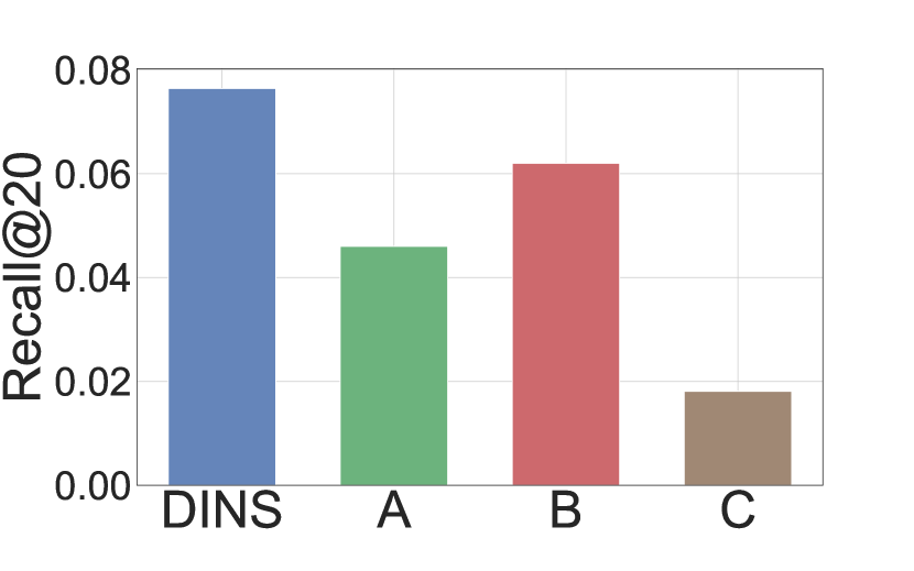
In this section, we conduct an ablation study of the three modules of DINS on LightGCN by building variants. A is built by removing the Hard Boundary Definition module, where we randomly sample a boundary item from the candidate set. B is built by replacing the dimension independent mixup module with the traditional mixup. C is built by removing the multi-hop pooling module by only considering the negative item for the first layer aggregation. Corresponding experimental results are presented in Figure 4. We can have the following observations:
-
•
DINS always performs the best. Removing any module would have a negative effect on the performance. It reveals each part of DINS contributes to the performance.
-
•
Removing the Hard Boundary Definition module (Variant A) results in a substantial drop in performance across the datasets, indicating the importance of maintaining an optimal size for the negative sampling region. A too-small region may lead to the loss of valuable feature information from the negative samples. At the same time, a too-large region hampers the effective fusion of information from the positive samples.
-
•
Compared with the other two modules, changing the dimension independent mixup module to the traditional mixup (Variant B) has a relatively small performance drop. It shows the mixup technique is already powerful by generating negative items in the continuous space. The proposed dimension independent mixup further enhances the improvement, especially on the Alibaba.
-
•
Removing the multi-hop pooling module has a great impact on the performance. It reveals the importance of considering high-order information during the negative sampling procedure. This observation aligns with the finding of MixGCF (Huang et al., 2021).
By observing the data, it can be seen that the area of negative sampling can neither be too large nor too small. According to Equation 4, if the area is too small, the hard negative item is synthesized too close to the positive items and thus the features of the negatives will be lost, while if the area is too far, the features of the positive items cannot be incorporated into the hard negative items at all.


4.4. RQ3: Parameter Sensitivity
In this section, we focus on how the hyper-parameters (, ) and the boundary item selection method actually affect DINS.
4.4.1. Impact of the value
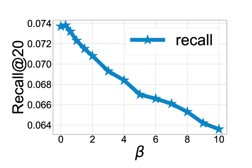
is a distinctive hyper-parameter within our DINS framework, serving to regulate the incorporation of information from the positive item as a collective entity into our synthetic hard negative item. is a propensity coefficient that controls whether our synthetic Hard Negative Samples (HNS) as a whole converge toward positive or negative items. Larger means the synthetic HNS is closer to the positive item. We conduct experiments with all datasets on recommenders. Due to the space limit, we illustrate parts of the results in Figure 5. Similar trends are also observed in other experiments.
-
•
As the dataset becomes sparser, the encoder necessitates the fusion of a greater amount of information about the positive items. According to the statistics in Table 1, it is clear that Yelp2018 is much denser than Amazon and Alibaba. On the Yelp2018 dataset, LightGCN achieved the best results at around and MF at around . In contrast, on the Amazon dataset, LightGCN needs to be around 2.3 and MF needs to be around 8 to achieve the best results. This may be due to the fact that the sparser the dataset the more uniform the embedding distribution of users and items is, resulting in a larger sampling boundary for determination. Even after dimension-wise mixup, the synthesized negative items can still be far away from the positive one, so we need to move closer to the positive item as a whole with a larger bet.
-
•
The stronger the encoding capability of the encoder, the less information from the positive item is needed for DINS. LightGCN is a state-of-the-art CF method that employs a message-passing mechanism on the bipartite user-item graph to learn a better embedding and MF is a straightforward model which recommends by a factorization-based approach. The -values required for LightGCN to achieve the best performance on all three datasets are much smaller than those of MF. This may be because LightGCN uses a message-passing mechanism on the graph to automatically aggregate a portion of the information from the positive items, while MF does not have a message-passing mechanism to naturally aggregate the information from the positives.
4.4.2. Impact of the candidate set size
We also conducted an experimental analysis on the candidate set size for negative items in DNS and MixGCF. Then we tested these baselines using candidate set sizes of 8, 16, 32, and 64. Detail experiments are illustrated in Figure 6. We can observe that the impacts all the sampling methods. Generally, increasing the candidate set size tends to improve the performance of the experiment. For example, the best results are mostly achieved with . Interestingly, MixGCF exhibits lower stability than DNS and DINS, even yielding contrasting outcomes on the Amazon dataset. Notably, as the candidate set increases, MixGCF demonstrates a significant decline. We attribute this disparity in results to the attributes of the dataset.
4.4.3. Impact of the boundary item selection method.
To delve deeper into the influence of the boundary item selection method in Section 3.1, we further conduct experiments on the impact of the selection method. In the experiment, we opt for LightGCN as the encoder due to its superior performance. To be noted that the sampled boundary item decides the sampling area together with the positive item. The area is the continuous space between the boundary and the positive item. By multiplying all the absolute differences in each dimension, we can obtain the volume of the sampling area. Based on this principle, we further design sampling methods to find the boundary item as:
-
•
Random. Randomly select an item from the candidate set as the boundary item.
-
•
Min. Find the item that constitutes the minimum sampling area volume as the boundary item.
-
•
Max. Find the item that constitutes the maximum sampling area volume as the boundary item.
-
•
Dot Product (DP). The method used in DINS as Equation 3.
After obtaining the boundary item, we also conduct the dimension independent mixup and multi-hop pooling. Subsequently, we conducted experiments on LightGCN to examine the impact of the boundary item selection method across the three datasets. The detailed experimental results are shown in Table 3. We can observe that Min and Max perform badly in most cases, which reveals the importance of selecting a suitable area for generating negative items. Even random selection outperforms Min and Max methods. The method used by DINS (DP) always performs the best across the datasets. It shows we have selected a suitable sampling area to generate the negative item.
| Amazon | Alibaba | Yelp2018 | ||||
| R@20 | N@20 | R@20 | N@20 | R@20 | N@20 | |
| Random | 0.0300 | 0.0123 | 0.0460 | 0.0201 | 0.0653 | 0.0537 |
| Min | 0.0145 | 0.0055 | 0.0279 | 0.0129 | 0.0441 | 0.0360 |
| Max | 0.0246 | 0.0084 | 0.0182 | 0.0081 | 0.0357 | 0.0294 |
| DP | 0.0493 | 0.0231 | 0.0764 | 0.0358 | 0.0738 | 0.0606 |
4.5. RQ4: Case Study
To answer RQ4: Does DINS really support area-wise hard negative sampling? we conduct a case study for readers to understand the sampling principle behind DINS. Experiments are conducted on the Yelp2018 dataset with LightGCN as the backbone recommender. We train the model with RNS, MixGCF, and DINS for epochs. For a fixed user-item interaction, we store the embedding of the positive item and the sampled negative item by different sampling methods in each iteration. Then we obtain the averaged positive item representation by mean pooling over all the collected positive item embedding. Then we concatenate the averaged positive item and all collected negative items embedding together and visualize the distribution via t-SNE (Van der Maaten and Hinton, 2008). For better visualization, we move the positive item to the center of the visualization by subtracting all the reduced -d embedding from the reduced positive item embedding.
The visualization is shown in Figure 7. We draw a circle (with a radius represented by ) to show the farthest sampled negative item. We can have three observations:
-
•
The RNS sampling method samples varied negative items that are far from the positive item. It exhibits the characteristic of the point-wise negative sampling method. It samples other existing items that are restricted in the upper-left corner area based on currently learned embedding.
-
•
The MixGCF method, as expected for the line-wise sampling method, exhibits line-style negative sampling results. It is due to the traditional Mixup method that generates a linear interpolation of two embeddings with the same weight on all dimensions.
-
•
DINS shows the characteristics of the area-wise sampling method. We can observe the sampled negative items spans across the whole circle, which gives a sufficient exploration of the embedding space. At the same time, the sample radius of DINS is only , which is the smallest among the three methods. It shows DINS samples the hard negatives for assist model training.


5. Related Work
In this section, we introduce the related work for DINS, which includes the graph-based recommendation and negative sampling method in recommendation.
5.1. Graph-based recommendation
Recent years have witnessed the rapid development of the emerging direction of GNN-based recommender systems (He et al., 2020; Peng et al., 2022; Wang et al., 2019; Ying et al., 2018; van den Berg et al., 2017; Yang et al., 2021, 2022; Wang et al., 2022; Yang et al., 2023b) where the user-item interactions are presented as a bipartite graph, and graph neural network methods are employed to learn the representation of each node via exploring structure information. For example, Pinsage (Ying et al., 2018) samples neighborhoods according to the visit counts of a node through a random-walk sampling approach. GC-MC (van den Berg et al., 2017) proposes a graph auto-encoder framework to construct the node representation by directly aggregating the information of its neighbors. NGCF (Wang et al., 2019) captures high-order connectivities by stacking multiple embedding propagation layers and utilizes the combination of different layers’ output for the rating prediction. Compared with NGCF, LightGCN (He et al., 2020) achieves better training efficiency and generation capability by removing the feature transformation and nonlinear activation function. Finally, SVD-GCN (Peng et al., 2022) further simplifies LightGCN by replacing neighborhood aggregation with exploiting K-largest singular vectors for the close relation between GCN-based and low-rank methods.
5.2. Negative sampling method
Negative sampling methods in RecSys have gained significant attention due to their ability to accelerate training and greatly enhance model performance, which can be categorized into the following groups. Static Sampler usually selects negatives from items that the user has not interacted with yet, based on a pre-defined distribution, like uniformity distribution (He et al., 2020; Wang et al., 2019; Rendle et al., 2012) or popularity distribution (Chen et al., 2017b). Hard Negative Sampler techniques choose negative items with the highest scores from the current recommender (Zhang et al., 2013; Shi et al., 2022). There are some mixup-based methods (Huang et al., 2021; Lai et al., 2023) generate new negative items by performing mix operations. GAN-based methods like IRGAN(Wang et al., 2017) and AdvIR(Park and Chang, 2019) use adversarial learning to generate negative items and improve robustness. Auxiliary-based Samplers leverage additional information, such as the knowledge graph in KGPolicy(Wang et al., 2020) or Personalized PageRank scores in PinSage(Ying et al., 2018), to sample hard negative instances.
6. Conclusion
In conclusion, this paper provides a novel perspective to revisit the current negative sampling methods based on continuous sampling area and classifies them into point-wise and line-wise sampling methods. In a further step, we design the first area-wise sampling method, named DINS, by proposing the Dimension Independent Mixup method. DINS can easily support both matrix factorization and graph-based backbone recommenders. Extensive experiments demonstrate superior performance compared with other methods, making it a state-of-the-art solution for negative sampling when training collaborative filtering with implicit feedback. The contributions of this work include a fresh perspective on negative sampling methods, the introduction of Area-wise sampling, and the development of the innovative DINS method. These findings have the potential to enhance RecSys capabilities and improve user experiences in various online services.
Acknowledgements.
This work is supported by Hebei Natural Science Foundation of China Grant F2022203072, CCF-Zhipu AI Large Model Fund (CCF-Zhipu202307), Innovation Capability Improvement Plan Project of Hebei Province (22567626H), supported in part by NSF under grants III-1763325, III-1909323, III-2106758, and SaTC-1930941.References
- (1)
- Chae et al. (2018) Dong-Kyu Chae, Jin-Soo Kang, Sang-Wook Kim, and Jung-Tae Lee. 2018. Cfgan: A generic collaborative filtering framework based on generative adversarial networks. In Proceedings of the 27th ACM international conference on information and knowledge management. 137–146.
- Chen et al. (2023) Chong Chen, Weizhi Ma, Min Zhang, Chenyang Wang, Yiqun Liu, and Shaoping Ma. 2023. Revisiting negative sampling vs. non-sampling in implicit recommendation. ACM Transactions on Information Systems 41, 1 (2023), 1–25.
- Chen et al. (2017a) Ting Chen, Yizhou Sun, Yue Shi, and Liangjie Hong. 2017a. On sampling strategies for neural network-based collaborative filtering. In Proceedings of the 23rd ACM SIGKDD International Conference on Knowledge Discovery and Data Mining. 767–776.
- Chen et al. (2017b) Ting Chen, Yizhou Sun, Yue Shi, and Liangjie Hong. 2017b. On Sampling Strategies for Neural Network-Based Collaborative Filtering. In Proceedings of the 23rd ACM SIGKDD International Conference on Knowledge Discovery and Data Mining (Halifax, NS, Canada) (KDD ’17). Association for Computing Machinery, New York, NY, USA, 767–776. https://doi.org/10.1145/3097983.3098202
- Chen et al. (2018) Yian Chen, Xing Xie, Shou-De Lin, and Arden Chiu. 2018. WSDM cup 2018: Music recommendation and churn prediction. In Proceedings of the Eleventh ACM International Conference on Web Search and Data Mining. 8–9.
- Ding et al. (2020a) Jingtao Ding, Yuhan Quan, Quanming Yao, Yong Li, and Depeng Jin. 2020a. Simplify and Robustify Negative Sampling for Implicit Collaborative Filtering. In Advances in Neural Information Processing Systems, H. Larochelle, M. Ranzato, R. Hadsell, M.F. Balcan, and H. Lin (Eds.), Vol. 33. Curran Associates, Inc., 1094–1105.
- Ding et al. (2020b) Jingtao Ding, Yuhan Quan, Quanming Yao, Yong Li, and Depeng Jin. 2020b. Simplify and robustify negative sampling for implicit collaborative filtering. Advances in Neural Information Processing Systems 33 (2020), 1094–1105.
- Glorot and Bengio (2010) Xavier Glorot and Yoshua Bengio. 2010. Understanding the difficulty of training deep feedforward neural networks. In International Conference on Artificial Intelligence and Statistics. 249–256.
- Gu et al. (2020) Yulong Gu, Zhuoye Ding, Shuaiqiang Wang, and Dawei Yin. 2020. Hierarchical user profiling for e-commerce recommender systems. In Proceedings of the 13th International Conference on Web Search and Data Mining. 223–231.
- He et al. (2020) Xiangnan He, Kuan Deng, Xiang Wang, Yan Li, Yong Dong Zhang, and Meng Wang. 2020. LightGCN: Simplifying and Powering Graph Convolution Network for Recommendation. SIGIR 2020 - Proceedings of the 43rd International ACM SIGIR Conference on Research and Development in Information Retrieval. https://doi.org/10.1145/3397271.3401063
- Huang et al. (2021) Tinglin Huang, Yuxiao Dong, Ming Ding, Zhen Yang, Wenzheng Feng, Xinyu Wang, and Jie Tang. 2021. MixGCF: An Improved Training Method for Graph Neural Network-based Recommender Systems. Proceedings of the 27th ACM SIGKDD Conference on Knowledge Discovery & Data Mining (2021).
- Kingma and Ba (2014) Diederik P. Kingma and Jimmy Lei Ba. 2014. Adam: A Method for Stochastic Optimization.. In International Conference on Learning Representations.
- Koren et al. (2021) Yehuda Koren, Steffen Rendle, and Robert Bell. 2021. Advances in collaborative filtering. Recommender systems handbook (2021), 91–142.
- Lai et al. (2023) Riwei Lai, Li Chen, Yuhan Zhao, Rui Chen, and Qilong Han. 2023. Disentangled Negative Sampling for Collaborative Filtering. In Proceedings of the Sixteenth ACM International Conference on Web Search and Data Mining (Singapore, Singapore) (WSDM ’23). Association for Computing Machinery, New York, NY, USA, 96–104. https://doi.org/10.1145/3539597.3570419
- Liu et al. (2021) Ye Liu, Kazuma Hashimoto, Yingbo Zhou, Semih Yavuz, Caiming Xiong, and Philip S Yu. 2021. Dense hierarchical retrieval for open-domain question answering. arXiv preprint arXiv:2110.15439 (2021).
- Mao et al. (2021) Kelong Mao, Jieming Zhu, Jinpeng Wang, Quanyu Dai, Zhenhua Dong, Xi Xiao, and Xiuqiang He. 2021. SimpleX: A simple and strong baseline for collaborative filtering. In Proceedings of the 30th ACM International Conference on Information & Knowledge Management. 1243–1252.
- Mayer-Schönberger and Cukier (2013) Viktor Mayer-Schönberger and Kenneth Cukier. 2013. Big data: A revolution that will transform how we live, work, and think. Houghton Mifflin Harcourt.
- Mikolov et al. (2013) Tomas Mikolov, Ilya Sutskever, Kai Chen, Greg Corrado, and Jeffrey Dean. 2013. Distributed Representations of Words and Phrases and Their Compositionality. In Proceedings of the 26th International Conference on Neural Information Processing Systems - Volume 2 (Lake Tahoe, Nevada) (NIPS’13). Curran Associates Inc., Red Hook, NY, USA, 3111–3119.
- Park and Chang (2019) Dae Hoon Park and Yi Chang. 2019. Adversarial sampling and training for semi-supervised information retrieval. In The World Wide Web Conference. 1443–1453.
- Peng et al. (2022) Shaowen Peng, Kazunari Sugiyama, and Tsunenori Mine. 2022. SVD-GCN: A Simplified Graph Convolution Paradigm for Recommendation. In Proceedings of the 31st ACM International Conference on Information & Knowledge Management, Atlanta, GA, USA, October 17-21, 2022, Mohammad Al Hasan and Li Xiong (Eds.). ACM, 1625–1634.
- Rendle and Freudenthaler (2014) Steffen Rendle and Christoph Freudenthaler. 2014. Improving pairwise learning for item recommendation from implicit feedback. In Proceedings of the 7th ACM international conference on Web search and data mining. 273–282.
- Rendle et al. (2012) Steffen Rendle, Christoph Freudenthaler, Zeno Gantner, and Lars Schmidt-Thieme. 2012. BPR: Bayesian personalized ranking from implicit feedback. In Conference on Uncertainty in Artificial Intelligence.
- Shi et al. (2022) Kexin Shi, Yun Zhang, Bingyi Jing, and Wenjia Wang. 2022. Soft BPR Loss for Dynamic Hard Negative Sampling in Recommender Systems. arXiv preprint arXiv:2211.13912 (2022).
- van den Berg et al. (2017) Rianne van den Berg, Thomas N. Kipf, and Max Welling. 2017. Graph Convolutional Matrix Completion. CoRR abs/1706.02263 (2017).
- Van der Maaten and Hinton (2008) Laurens Van der Maaten and Geoffrey Hinton. 2008. Visualizing data using t-SNE. Journal of machine learning research 9, 11 (2008).
- Wang et al. (2017) Jun Wang, Lantao Yu, Weinan Zhang, Yu Gong, Yinghui Xu, Benyou Wang, Peng Zhang, and Dell Zhang. 2017. IRGAN: A Minimax Game for Unifying Generative and Discriminative Information Retrieval Models. In Annual International ACM SIGIR Conference on Research and Development in Information Retrieval. 515–524.
- Wang et al. (2022) Shen Wang, Liangwei Yang, Jibing Gong, Shaojie Zheng, Shuying Du, Zhiwei Liu, and S Yu Philip. 2022. MetaKRec: Collaborative Meta-Knowledge Enhanced Recommender System. In 2022 IEEE International Conference on Big Data (Big Data). IEEE, 665–674.
- Wang et al. (2019) Xiang Wang, Xiangnan He, Meng Wang, Fuli Feng, and Tat-Seng Chua. 2019. Neural Graph Collaborative Filtering. Proceedings of the 42nd International ACM SIGIR Conference on Research and Development in Information Retrieval (2019).
- Wang et al. (2020) Xiang Wang, Yaokun Xu, Xiangnan He, Yixin Cao, Meng Wang, and Tat-Seng Chua. 2020. Reinforced Negative Sampling over Knowledge Graph for Recommendation. In WWW.
- Wu et al. (2019) Chuhan Wu, Fangzhao Wu, Mingxiao An, Jianqiang Huang, Yongfeng Huang, and Xing Xie. 2019. NPA: neural news recommendation with personalized attention. In Proceedings of the 25th ACM SIGKDD international conference on knowledge discovery & data mining. 2576–2584.
- Wu et al. (2021) Jiancan Wu, Xiang Wang, Fuli Feng, Xiangnan He, Liang Chen, Jianxun Lian, and Xing Xie. 2021. Self-supervised graph learning for recommendation. In Proceedings of the 44th international ACM SIGIR conference on research and development in information retrieval. 726–735.
- Yang et al. (2021) Liangwei Yang, Zhiwei Liu, Yingtong Dou, Jing Ma, and Philip S Yu. 2021. Consisrec: Enhancing gnn for social recommendation via consistent neighbor aggregation. In Proceedings of the 44th international ACM SIGIR conference on Research and development in information retrieval. 2141–2145.
- Yang et al. (2022) Liangwei Yang, Zhiwei Liu, Yu Wang, Chen Wang, Ziwei Fan, and Philip S Yu. 2022. Large-scale personalized video game recommendation via social-aware contextualized graph neural network. In Proceedings of the ACM Web Conference 2022. 3376–3386.
- Yang et al. (2023b) Liangwei Yang, Shengjie Wang, Yunzhe Tao, Jiankai Sun, Xiaolong Liu, Philip S Yu, and Taiqing Wang. 2023b. DGRec: Graph Neural Network for Recommendation with Diversified Embedding Generation. In Proceedings of the Sixteenth ACM International Conference on Web Search and Data Mining. 661–669.
- Yang et al. (2023a) Zhen Yang, Ming Ding, Xu Zou, Jie Tang, Bin Xu, Chang Zhou, and Hongxia Yang. 2023a. Region or Global? A Principle for Negative Sampling in Graph-Based Recommendation. IEEE Transactions on Knowledge and Data Engineering 35, 6 (2023), 6264–6277. https://doi.org/10.1109/TKDE.2022.3155155
- Ying et al. (2018) Rex Ying, Ruining He, Kaifeng Chen, Pong Eksombatchai, William L Hamilton, and Jure Leskovec. 2018. Graph convolutional neural networks for web-scale recommender systems. In Proceedings of the 24th ACM SIGKDD international conference on knowledge discovery & data mining. 974–983.
- Zhang et al. (2023) Dan Zhang, Yifan Zhu, Yuxiao Dong, Yuandong Wang, Feng Wenzheng, Evgeny Kharlamov, and Jie Tang. 2023. ApeGNN: Node-Wise Adaptive Aggregation in GNNs for Recommendation. In WWW’23.
- Zhang et al. (2018) Hongyi Zhang, Moustapha Cissé, Yann N. Dauphin, and David Lopez-Paz. 2018. mixup: Beyond Empirical Risk Minimization. In 6th International Conference on Learning Representations, ICLR 2018, Vancouver, BC, Canada, April 30 - May 3, 2018, Conference Track Proceedings.
- Zhang et al. (2013) Weinan Zhang, Tianqi Chen, Jun Wang, and Yong Yu. 2013. Optimizing top-n collaborative filtering via dynamic negative item sampling. In Annual International ACM SIGIR Conference on Research and Development in Information Retrieval.
- Zhen et al. (2020) Yang Zhen, Ding Ming, Zhou Chang, Yang Hongxia, Zhou Jingren, and Tang Jie. 2020. Understanding Negative Sampling in Graph Representation Learning. (2020), 1666–1676.
- Zheng et al. (2019) Lei Zheng, Chaozhuo Li, Chun-Ta Lu, Jiawei Zhang, and Philip S Yu. 2019. Deep Distribution Network: Addressing the Data Sparsity Issue for Top-N Recommendation. In Proceedings of the 42nd International ACM SIGIR Conference on Research and Development in Information Retrieval. 1081–1084.