Diffusive limit of non-Markovian quantum jumps

Deriving and solving the equations of motion for driven dissipative quantum systems is a notoriously hard task, especially in the presence of quantum memory effects. In this Letter, we open new avenues to tackle these problems of broad on-going interest. Currently, state-of-the-art experiments explore driven dissipative open quantum systems Bloch et al. (2008), non-equilibrium phase transitions in a Rydberg gas has been observed Gutiérrez et al. (2017), simulation of general open system dynamics with trapped ions has been reported Barreiro et al. (2011); Müller et al. (2011) – and even the statistical likelihood of a physical process (a statistical arrow of time) has been experimentally characterized using superconducting qubit systems Harrington et al. (2019). Similar type of open quantum systems appear also in the context of photosynthesis Engel et al. (2007); Lee et al. (2007) and in general in molecular aggregates Brixner et al. .

One of the main difficulties in analyzing driven open quantum systems has its origin in the lack of a typical time scale, such as an energy gap of the system Hamiltonian. One possible solution is to try to model the open system and environment dynamics exactly, as in non-Markovian quantum state diffusion Diósi et al. (1998); Strunz et al. (1999), where a stochastic Schrödinger equation describes the dynamics of the open system and the effects of the environment are contained in the statistical properties of the driving noise. Typically approximation methods are required to solve the resulting equations of motion Yu et al. (1999); Suess et al. (2014); Hartmann and Strunz (2017). This type of approach has been successfully used to describe energy Roden et al. (2009); Ritschel et al. (2011); Abramavicius and Abramavicius (2014) and charge transport Gao and Eisfeld (2019); Zhong and Zhao (2013) in molecular aggregates.

Alternatively, starting from a microscopic model an effective time local master equation can be derived Breuer et al. (2002) and unravelled, for example, with non-Markovian quantum jumps Piilo et al. (2008, 2009); Härkönen (2010). Quantum jump methods have been used earlier, e.g., to study excitonic energy transport with Ai et al. (2014); Tao et al. (2016) and without driving Rebentrost et al. (2009); Oh et al. (2019) and even to understand singlet fission in molecular crystals, which may help to design more efficient solar panels Renaud and Grozema (2015).

On the theoretical side, our motivation is to look for the missing connection between the quantum jump Piilo et al. (2008) and quantum state diffusion Strunz et al. (1999) approaches in the non-Markovian regime – and with the help of these results expand significantly their applicability of the former for complex practical problems. First, we formulate both approaches in the projective Hilbert space, thus extending the well known results from the Markov Breuer and Petruccione (1995) to the non-Markovian regime. Then a diffusive limit of the quantum jumps is taken in such a way that it coincides with quantum state diffusion in the projective Hilbert space and in the non-Markovian regime. Interestingly, the same limit in Hilbert space results in a completely new unraveling, which we call non-Markovian quantum diffusion (see Fig. 1). We enhance the quantum jumps and quantum diffusion approaches with kernel smoothing techniques Ghosh (2017), which allows us to handle driven dissipative systems with quantum memory effects easily. Lastly, we apply all of the methods to the driven dissipative two level atom.

A typical model for open systems in the interaction picture with respect to environment Hamiltonian $H_{B}=\sum_{\lambda}\omega_{\lambda}a_{\lambda}^{\dagger}a_{\lambda}$ is

$\displaystyle H(t)=$

$\displaystyle H_{S}(t)+\sum_{\lambda}g_{\lambda}La_{\lambda}^{\dagger}e^{i\omega_{\lambda}t}+g_{\lambda}^{*}L^{\dagger}a_{\lambda}e^{-i\omega_{\lambda}t},$

(1)

where the creation- and annihilation operators $a_{\lambda}^{\dagger}$ and $a_{\lambda}$ of a bath mode labeled by $\lambda$ satisfy the bosonic commutation relations $[a_{\lambda},a_{\mu}^{\dagger}]=\delta_{\lambda\mu}$. We assume that the coupling operator $L$ is traceless, i.e. $\text{tr}\left\{L\right\}{}=0$.

In a projective Hilbert space $\mathcal{P}(\mathcal{H})$, each point is associated with a projector $|\psi\rangle\!\langle\psi|$ Breuer et al. (2002); Chruscinski and Jamiolkowski (2004). Given a separable Hilbert space, coordinates $\psi_{i}\in\mathbb{C}$ on a $\mathcal{P}(\mathcal{H})$ can be easily constructed with respect to a fixed orthonormal basis as $|\psi\rangle=\sum_{i}\psi_{i}|i\rangle$. For more information on $\mathcal{P}(\mathcal{H})$, see the Supplementary Material Note (1).

Reduced system dynamics can be represented exactly for a large class of models, even beyond Eq. (1) Link and Strunz (2017), with the following linear non-Markovian quantum state diffusion (NMQSD) equation

	$\displaystyle\partial_{t}|\psi(t,z^{*})\rangle=$	$\displaystyle\left[-iH_{S}(t)+z_{t}^{*}L\right]|\psi(t,z^{*})\rangle$
		$\displaystyle-L^{\dagger}\int\limits_{0}^{t}\textrm{d}s\,\alpha(t-s)\frac{\delta|\psi(t,z^{*})\rangle}{\delta z_{s}^{*}}.$		(2)

Here, $L$ is the coupling operator between the system and the bath and $H_{S}(t)$ is an arbitrary Hamiltonian acting on the open system Diósi et al. (1998); Strunz et al. (1999). NMQSD is driven by a complex valued colored Gaussian noise $z_{t}^{*}$, completely characterized by the correlations

$\displaystyle\mathsf{M}\left[z_{t}z_{s}^{*}\right]=\alpha(t-s),\qquad\mathsf{M}\left[z_{t}^{*}\right]=\mathsf{M}\left[z_{t}z_{s}\right]=0,$

(3)

where $\mathsf{M}\left[\cdot\right]$ is the average over the noise process $z_{t}^{*}$. Solutions $|\psi(t,z^{*})\rangle$ are analytic functionals of the whole noise process $z_{t}^{*}$ up to time $t$.

In the remainder of this Letter, we will make the following restriction. We assume that the functional derivative satisfies, at least approximately Yu et al. (1999)

$\displaystyle\frac{\delta}{\delta z_{s}^{*}}|\psi(z^{*},t)\rangle=f(t,s)L|\psi(z^{*},t)\rangle.$

(4)

Eq. (4) guarantees that the mean state will evolve according to a closed form master equation. However, the NMQSD method itself works perfectly well even if no such master equation exist for the reduced state.

The above stochastic Schrödinger equation (Non-Markovian quantum state diffusion.—) satisfies the ordinary rules of calculus since the noise process has a finite correlation time. The dynamics of the average state $\rho(t)=\mathsf{M}\left[|\psi(z^{*},t)\rangle\!\langle\psi(z^{*},t)|\right]$ described by Eq. (Non-Markovian quantum state diffusion.—) with assumption (4) reads

	$\displaystyle\dot{\rho}(t)$	$\displaystyle=-i[H_{S}(t)+S(t)L^{\dagger}L,\rho(t)]+2\gamma(t)L\rho(t)L^{\dagger}$
		$\displaystyle-\gamma(t)\left\{L^{\dagger}L,\rho(t)\right\},$		(5)

where $F(t)=\gamma(t)+iS(t)$ and $F(t)=\int_{0}^{t}\textrm{d}s\,\alpha(t-s)f(t,s)$.

To look for a connection between NMQSD and non-Markovian quantum jumps, we first have to derive a representation of the former in the projective Hilbert space. The probability density functional can be expressed as

$\displaystyle P_{Q}[\psi,t]$

$\displaystyle=\mathsf{M}\left[\delta(\psi-\psi(z^{*},t))\right].$

(6)

We show in Sec. LABEL:sec:deriv-fokk-planck of ¹¹1Supplementary Material, that the probability density functional satisfies the following second order partial differential equation

	$\displaystyle\partial_{t}P_{Q}[\psi,t]=$	$\displaystyle\sum_{k=1}^{d}\partial_{\psi_{k}}c_{k}(\psi)P_{Q}[\psi,t]+\partial_{\psi_{k}^{*}}c_{k}^{*}(\psi)P_{Q}[\psi,t]$
		$\displaystyle+\sum_{k,l=1}^{d}\partial^{2}_{\psi_{k}\psi_{l}^{*}}d_{kl}(\psi)P_{Q}[\psi,t],$		(7)

where the drift and diffusion coefficients are $c_{k}(\psi)=\langle k|\left(-iH-F(t)L^{\dagger}L\right)|\psi\rangle$ and $d_{kl}(\psi)=\left(F(t)+F^{*}(t)\right)\langle k|L|\psi\rangle\langle\psi|L^{\dagger}|l\rangle$, respectively. NMQSD thus corresponds to a $2$nd order Kramers - Moyal expansion in $\mathcal{P}(\mathcal{H})$ Risken (2012). If the diffusion coefficient $F(t)+F^{*}(t)=2\gamma(t)$ is not negative for any time $t$ the KME² equation is, in fact, a proper Fokker-Planck equation Gardiner (2009).

Master equations of the form

	$\displaystyle\dot{\rho}(t)=$	$\displaystyle-i[H_{S}(t)+\sum_{k}s_{k}(t)L_{k}^{\dagger}L_{k},\rho]+\sum_{k}2\gamma_{k}(t)L_{k}\rho L_{k}^{\dagger}$
		$\displaystyle-\gamma_{k}(t)\left\{L_{k}^{\dagger}L_{k},\rho(t)\right\},$		(8)

can be unravelled with non-Markovian quantum jumps (NMQJ) Piilo et al. (2008, 2009); Härkönen (2010), ²²2We demand that at time $t=0$ all of the decay rates $\gamma_{k}(t)$ have to be non-negative. It is a piecewise deterministic process in the Hilbert space of the open system. Here we present a linear version of the process (LNMQJ) given by the following Ito stochastic differential equation

	$\displaystyle|\textrm{d}\psi\rangle=$	$\displaystyle-iG(t)|\psi\rangle\textrm{d}t+\sum_{k}(L_{k}-\mathbbm{1})|\psi\rangle\textrm{d}N_{+}^{k}(t)$
		$\displaystyle+\int\textrm{d}\psi^{\prime}\,\left(|\psi^{\prime}\rangle-|\psi\rangle\right)\textrm{d}N_{-,\psi^{\prime}}^{k}(t),$		(9)

where $G(t)=H_{S}(t)+\sum_{k}s_{k}(t)L_{k}^{\dagger}L_{k}-i\gamma_{k}(t)[L_{k}^{\dagger}L_{k}-\mathbbm{1}]$. Increments of the Poisson processes, $\textrm{d}N_{+}^{k}(t)$ and $\textrm{d}N_{-,\psi^{\prime}}^{l}(t),$ are mutually independent $\textrm{d}N_{+}^{k}(t)\textrm{d}N_{+}^{l}(t)=\delta_{kl}\textrm{d}N_{+}^{k}(t)$, $\textrm{d}N_{-,\psi^{\prime}}^{k}(t)\textrm{d}N_{-,\psi^{\prime\prime}}^{l}(t)=\delta_{kl}\delta(\psi^{\prime}-\psi^{\prime\prime})\textrm{d}N_{-,\psi^{\prime}}(t)$ and $\textrm{d}N_{+}^{k}(t)\textrm{d}N_{-,\psi^{\prime}}^{l}(t)=0$. The mean values of the increments are ${\mathsf{E}}\left[\textrm{d}N_{+}^{k}(t)\right]=2\gamma_{+}^{k}(t)\textrm{d}t$ and ${\mathsf{E}}\left[\textrm{d}N_{-,\psi^{\prime}}^{l}(t)\right]=2\gamma_{-}^{l}(t)\frac{P[\psi^{\prime},t]}{P[\psi,t]}\delta(\psi-L_{l}\psi^{\prime})\textrm{d}t$, where $\gamma_{k}(t)=\gamma_{k}^{+}(t)-\gamma_{k}^{-}(t)$. It is easy to see that the average evolution reproduces Eq. (Non-Markovian Quantum Jumps.—).

In NMQJ, the memory effects reside in the jump probability from a source state $\psi$ to a target state $\psi^{\prime}$ via channel $k$ when $\gamma_{k}(t)<0$. In particular, a “reverse jump” can occur from $\psi$ to $\psi^{\prime}$ iff $L_{k}|\psi^{\prime}\rangle=|\psi\rangle$. The probability of such jumps depends on the ratio $P[\psi^{\prime},t]/P[\psi,t]$. In order to compute the jump probability, the knowledge of the whole ensemble is required Piilo et al. (2008). This poses a serious challenge since a state $|\psi\rangle\!\langle\psi|$ has measure zero in $\mathcal{P}(\mathcal{H})$. We describe later a method to overcome this.

Now, Eq. (Non-Markovian quantum state diffusion.—) is equivalent to Eq. (Non-Markovian Quantum Jumps.—) with $2m\,(1\leq k\leq 2m)$ time dependent rates and time independent jump operators defined as

	$\displaystyle s_{k}(t)=$	$\displaystyle\frac{s(t)}{2m|\xi_{k}|^{2}\varepsilon^{2}},\qquad\gamma_{k}(t)=\frac{\gamma(t)}{2m|\xi_{k}|^{2}\varepsilon^{2}},$
	$\displaystyle L_{k}=$	$\displaystyle\mathbbm{1}+\varepsilon\xi_{k}L,\,\,{\rm s.t.}\,\xi_{k}+\xi_{k+m}=0,$		(10)

where $\xi_{k}\in\mathbb{C}$, $|\xi_{k}|=|\xi|$ and $\varepsilon>0$. The deterministic part $G(t)$ of the quantum jump process in Eq. (Non-Markovian Quantum Jumps.—) transforms under (Non-Markovian Quantum Jumps.—) to $G^{\prime}(t)=H_{S}(t)+s(t)L^{\dagger}L-i\gamma(t)L^{\dagger}L+\Theta(t)\mathbbm{1}$. The last term $\Theta(t)=\sum_{k=1}^{2m}\frac{s(t)}{2m|\xi_{k}|^{2}\varepsilon^{2}}$ is a global phase factor, which can be neglected. If $||\varepsilon L||<1$, then operators $L_{l}$ are invertible ³³3${L_{l}}^{-1}=\sum_{j=0}^{\infty}(-1\xi_{l}\varepsilon)^{j}L^{j}=\mathbbm{1}-\varepsilon\xi_{l}L+\mathcal{O}(\varepsilon^{2})$, when ${||\varepsilon L||}<1$.. In this case, the transformed statistics of the Poisson increments eventually become

	$\displaystyle{\mathsf{E}}\left[\textrm{d}N_{+}^{k}(t)\right]$	$\displaystyle=\frac{\gamma_{+}(t)}{m\varepsilon^{2}|\xi_{k}|^{2}}\textrm{d}t,$
	$\displaystyle{\mathsf{E}}\left[\textrm{d}N_{-,\psi^{\prime}}^{l}(t)\right]$	$\displaystyle=\frac{\gamma_{-}(t)}{m\varepsilon^{2}|\xi_{k}|^{2}}\frac{P[\psi^{\prime},t]}{P[\psi,t]}\frac{\delta(L_{l}^{-1}\psi-\psi^{\prime})}{|\det L_{l}||\det L_{l}^{\dagger}|}\textrm{d}t.$		(11)

Remarkably, after the transformation the increment $\textrm{d}N_{-,\psi^{\prime}}^{l}(t)$ does not depend on the target state of the jump,$|\psi^{\prime}\rangle$, anymore. This arises because a reverse jump corresponds to a mapping $|\psi\rangle\mapsto L_{l}^{-1}|\psi\rangle=|\psi^{\prime}\rangle$, i.e. the target state of the jump is given by the action of the inverse operator on the source state $|\psi\rangle$.

Therefore, we can write the transformed process as

	$\displaystyle|\textrm{d}\psi_{t}\rangle=$	$\displaystyle-iG^{\prime}(t)|\psi\rangle\textrm{d}t+\sum_{k}\Bigg{[}(L_{k}-\mathbbm{1})|\psi_{t}\rangle\textrm{d}M_{+}^{k}(t)$
		$\displaystyle+\left({L_{k}}^{-1}-\mathbbm{1}\right)|\psi_{t}\rangle\textrm{d}M_{-}^{k}(t)\Bigg{]},$		(12)

with mutually independent Poisson increments $\textrm{d}M_{\pm}^{k}$ with statistics ${\mathsf{E}}\left[\textrm{d}M_{+}^{k}(t)\right]=\frac{\gamma_{+}(t)}{m\varepsilon^{2}|\xi_{k}|^{2}}\textrm{d}t$ and ${\mathsf{E}}\left[\textrm{d}M_{-}^{k}(t)\right]=\frac{P[{L_{k}}^{-1}\psi,t]}{P[\psi,t]|\det L_{k}||\det L_{k}^{\dagger}|}\frac{\gamma_{-}(t)}{m\varepsilon^{2}|\xi_{k}|^{2}}\textrm{d}t$, which are just relabeled increments of Eq. (Non-Markovian Quantum Jumps.—). To assert that this equation is still valid, we compute the average evolution of $|\psi\rangle\!\langle\psi|$ which coincides with the master equation (Non-Markovian quantum state diffusion.—) (see Sec. LABEL:sec:average-evolution of the Note (1)).

It is worth stressing that when $\gamma_{k}(t)<0$, the quantum jumps are given by the inverse jump operator $L_{k}^{-1}$. Contrary to the original approach in Piilo et al. (2008), the quantum jumps and reverse quantum jumps are exactly inverses of each other. The quantum memory effects are contained in the probability for these jumps which still depends on the ratio $P[L_{k}^{-1}\psi,t]/P[\psi,t]$.

In the projective Hilbert space LNMQJ corresponds to the following Liouville master equation Härkönen (2010)

	$\displaystyle\partial_{t}P[\psi,t]$	$\displaystyle=i\sum_{k}\partial_{\psi_{k}}\left(\langle k|G^{\prime}(t)|\psi\rangle P[\psi,t]\right)$
		$\displaystyle-\partial_{\psi_{k}^{*}}\left(\langle\psi|G^{\prime\dagger}(t)|k\rangle P[\psi,t]\right)$
		$\displaystyle+\int\textrm{d}\phi\,\left(R[\psi|\phi]P[\phi,t]-R[\phi|\psi]P[\psi,t]\right),$		(13)

where the jump rates $R[\phi|\psi]$ are

	$\displaystyle R[\phi|\psi]=$	$\displaystyle\sum_{k=1}^{2m}\frac{\gamma_{+}(t)}{m\varepsilon^{2}|\xi_{k}|^{2}}\delta(\phi-L_{k}\psi)$
		$\displaystyle+\frac{\gamma_{-}(t)}{m\varepsilon^{2}|\varepsilon_{k}|^{2}}\frac{P[\phi,t]}{P[\psi,t]}\delta(\psi-L_{k}\phi).$		(14)

When comparing the drift terms in Fokker-Planck equation (Non-Markovian quantum state diffusion.—) and in the Liouville master equation (LNMQJ in projective Hilbert space.—), we see that they are equal. The jump part takes the form $\int\textrm{d}\phi\,\left(R[\psi|\phi]P[\phi,t]-R[\phi|\psi]P[\psi,t]\right)=\sum_{k=1}^{2m}\frac{\gamma(t)}{m\varepsilon^{2}|\xi_{k}|^{2}}F_{k}[\psi]-\frac{2\gamma(t)}{\varepsilon^{2}|\xi|^{2}}P[\psi,t]$, where

$\displaystyle F_{k}[\psi]=\frac{P[L_{k}^{-1}\psi,t]}{|\det L_{k}||\det L_{k}^{\dagger}|}.$

(15)

After expanding $F_{k}[\psi]$ to second order in $\varepsilon$ and assuming $m>2$ we find $\int\textrm{d}\phi\,\left(R[\psi|\phi]P[\phi,t]-R[\phi|\psi]P[\psi,t]\right){\to}$
$\sum_{k,l=0}^{d}\partial^{2}_{\psi_{k}\psi_{l}^{*}}\left(2\gamma(t)\langle k|L|\psi\rangle\langle\psi|L^{\dagger}|l\rangle P[\psi,t]\right)$, while $\epsilon\to 0$ ⁴⁴4For the computation we use the results of  Note (1) to compute the determinant, to expand the probability density, to expand a rational polynomial and choose $\xi_{k}=e^{i\frac{\pi}{m}(k-1)}$ with $m\geq 2$. We thus have proven the validity of the part $\mathrm{LME}\xrightarrow{\varepsilon\to 0}\mathrm{FPE}$ of the diagram in Fig. 1.

Next we take the above diffusion limit directly on the piecewise deterministic LNMQJ process in the Hilbert space. Full details can be found in the Supplement Note (1). First, Eq. (Non-Markovian Quantum Jumps.—) is expanded to first order in $\varepsilon$, resulting in

	$\displaystyle|\textrm{d}\psi_{t}\rangle=$	$\displaystyle-iG^{\prime}(t)|\psi\rangle\textrm{d}t+\sum_{k}\Bigg{[}\xi_{k}L|\psi_{t}\rangle\varepsilon\textrm{d}M_{+}^{k}(t)$
		$\displaystyle-\xi_{k}L|\psi_{t}\rangle\varepsilon\textrm{d}M_{-}^{k}(t)\Bigg{]}+\mathcal{O}(\varepsilon^{2}).$		(16)

We define new processes $\textrm{d}V_{\pm}^{k}=\varepsilon\textrm{d}M_{\pm}^{k}-\varepsilon E\left[\textrm{d}M_{\pm}^{k}\right]$ Pellegrini and Petruccione (2009) and by using the Ito rules, we have ${\mathsf{E}}\left[\textrm{d}V_{\pm}^{k}\right]=0$, ${\mathsf{E}}\left[\textrm{d}V_{-}^{k}\textrm{d}V_{+}^{l}\right]=0$ and ${\mathsf{E}}\left[\textrm{d}V_{+}^{k}\textrm{d}V_{+}^{l}\right]=\delta_{kl}(\varepsilon\textrm{d}V_{+}^{k}+\frac{\gamma_{+}(t)}{m|\xi_{k}|^{2}}\textrm{d}t)$. We then define $\lim_{\varepsilon\to 0}\textrm{d}V_{\pm}^{k}=\textrm{d}W_{\pm}^{k}$, where the increments $\textrm{d}W_{\pm}^{k}$ satisfy the following Ito rules

	$\displaystyle{\mathsf{E}}\left[\textrm{d}W_{\pm}^{k}\right]=0,\qquad{\mathsf{E}}\left[\textrm{d}W_{-}^{k}\textrm{d}W_{+}^{l}\right]=0,$
	$\displaystyle{\mathsf{E}}\left[\textrm{d}W_{+}^{k}\textrm{d}W_{+}^{l}\right]=\delta_{kl}\frac{\gamma_{+}(t)}{m|\xi_{k}|^{2}}\textrm{d}t,$		(17)
	$\displaystyle{\mathsf{E}}\left[\textrm{d}W_{-}^{k}\textrm{d}W_{-}^{l}\right]=\delta_{kl}\frac{\gamma_{-}(t)}{m|\xi_{k}|^{2}}\textrm{d}t.$

The goal is now to express the stochastic Schrödinger equation (Non-Markovian quantum diffusion.—) in terms of Wiener increments $\textrm{d}W_{\pm}^{k}$. After some simplification steps (detailed in the Supplement Note (1)), we find in the limit $\varepsilon\to 0$

	$\displaystyle|\textrm{d}\psi\rangle=$	$\displaystyle\bigg{(}-iG^{\prime}(t)+2\gamma_{-}(t)\sum_{n=0}^{d}\langle\psi|L^{\dagger}|n\rangle\frac{\partial\ln P[\psi,t]}{\partial\psi_{n}^{*}}L\bigg{)}|\psi\rangle\textrm{d}t$
		$\displaystyle+L|\psi\rangle\textrm{d}Z_{+}-L|\psi\rangle\textrm{d}Z_{-},$		(18)

where $\textrm{d}Z_{\pm}=\sum_{k}\xi_{k}\textrm{d}W_{\pm}^{k}$. The complex noise $\textrm{d}Z_{\pm}$ satisfies

	$\displaystyle{\mathsf{E}}\left[\textrm{d}Z_{\pm}\right]=0,\quad{\mathsf{E}}\left[\textrm{d}Z_{\pm}\textrm{d}Z_{\pm}\right]=0,$
	$\displaystyle{\mathsf{E}}\left[\textrm{d}Z_{\pm}\textrm{d}Z_{\pm}^{*}\right]=2\gamma_{\pm}(t)\textrm{d}t.$		(19)

The average evolution of NMQD equation (Non-Markovian quantum diffusion.—) corresponds to Eq. (Non-Markovian Quantum Jumps.—) as we show in the Supplement Note (1).

Interestingly, both noises $\textrm{d}Z_{\pm}$ couple to the system via $L$ but with a different phase. Nevertheless, both noise terms produce “sandwich” terms $2\gamma_{\pm}(t)L\rho L^{\dagger}\textrm{d}t$ on the average evolution. The drift term with logarithmic derivative compensates the term $2\gamma_{-}(t)L\rho L^{\dagger}\textrm{d}t$ on average such that the correct sandwich term $2(\gamma_{+}(t)-\gamma_{-}(t))L\rho L^{\dagger}\textrm{d}t$ emerges. The term proportional to the logarithmic derivative can be seen as the change in the stochastic entropy of the system which contributes to the deterministic evolution Seifert (2005).

A Gaussian kernel $K$ is defined

$\displaystyle K[\psi]=\frac{1}{\pi^{d+1}}e^{-||\psi||^{2}},|\psi\rangle\in\mathbb{C}^{d+1}.$

(20)

Given an ensemble of stochastic states $\{|\psi^{\nu}\rangle\}_{\nu=1}^{M}$, we estimate the probability density $P[\psi]$ in the projective Hilbert space with

$\displaystyle P_{\sigma}[\psi]=\frac{1}{M(\sigma^{2}\pi^{d+1})}\sum_{\nu=1}^{M}K[(\psi-\psi^{\nu})/\sigma],$

(21)

where $\sigma>0$ is a free parameter. A rule of thumb for choosing the variance is that $\sigma=M^{\frac{-1}{d+5}}$ Ghosh (2017), where $d$ is the real dimension of the underlying Hilbert space. Using the estimated density, we can compute the logarithmic derivative of the density appearing in Eq. (Non-Markovian quantum diffusion.—) as

$\displaystyle\frac{\partial\ln P_{\sigma}[\psi]}{\partial\psi_{n}^{*}}=-\frac{\sum_{\nu=1}^{M}e^{-||\psi_{n}-\psi_{n}^{\nu}||^{2}}\frac{\psi_{n}-\psi_{n}^{\nu}}{\sigma^{2}}}{\sum_{\nu=1}^{M}e^{-||\psi_{n}-\psi_{n}^{\nu}||^{2}}}=-\frac{\psi_{n}-\langle\langle\psi_{n}\rangle\rangle}{\sigma^{2}},$

(22)

where average $\langle\langle\cdot\rangle\rangle$ is taken with respect to distribution $p_{\sigma}=\frac{1}{\mathcal{Z}}e^{-\frac{||\psi-\psi^{\nu}||^{2}}{\sigma^{2}}}$, with $\mathcal{Z}=\sum_{\nu=1}^{M}e^{-||\psi_{n}-\psi_{n}^{\nu}||^{2}}$. Kernel estimation can be also used to evaluate the ratios $\frac{P_{\sigma}[\psi^{\prime}]}{P_{\sigma}[\psi]}=\frac{\sum_{\nu^{\prime}=1}^{M}K[(\psi^{\prime}-\psi^{\nu^{\prime}})/\sigma]}{\sum_{\nu=1}^{M}K[(\psi-\psi^{\nu})/\sigma]}$. Therefore, after performing the transformation (Non-Markovian Quantum Jumps.—) on the NMQJ and using the smoothed estimate for $P[\psi,t]$ we can compute the reverse jump probabilities easily. The reason for this simplification is that the target state of the jump is directly given by the inverse jump operator and the ratio of probabilities for the target and the source state to occur can be efficiently evaluated from the estimate.

An open system with $H_{S}=\frac{\omega}{2}\sigma_{z}+\frac{\Omega}{2}\sigma_{x}$ and $L=\sigma_{-}$ corresponds to an amplitude damped two level atom with driving and is not solvable in closed form. We assume that the bath correlation function takes the following exponential form

$\displaystyle\alpha(t,s)=g\frac{\Gamma}{2}e^{-i\omega_{c}(t-s)-\Gamma|t-s|},$

(23)

where $\Gamma$ is the inverse of the bath correlation time $\tau_{c}=\Gamma^{-1}$, $\omega_{c}$ is the bath resonance frequency and $g>0$ is a dimensionless parameter describing the overall system bath coupling strength. The limit $\Gamma\to\infty$ leads to a singular bath correlation function $\alpha(t,s)\to g\delta(t-s)$ and to a Gorini-Kossakowski-Sudarshan-Lindblad master equation with time independent decay rate $g$ Gorini et al. (1976); Lindblad (1976). The chosen correlation function can emerge from a microscopic model where the driven two level system is placed inside a leaky cavity near absolute zero temperature such that thermal excitations can be neglected. When the bath correlation time is short, Eq. (4) is approximately true Yu et al. (1999). Within this approximation the NMQSD equation takes the following form

	$\displaystyle\partial_{t}|\psi_{t}(z^{*})\rangle=$	$\displaystyle-iH_{S}|\psi_{t}(z^{*})\rangle+z_{t}^{*}\sigma_{-}|\psi_{t}(z^{*})\rangle$
		$\displaystyle-F(t)\sigma_{+}\sigma_{-}|\psi_{t}(z^{*})\rangle,$		(24)

with $\alpha(t,s)=\langle z_{t}z_{s}^{*}\rangle$ being the only non-zero correlation of the complex noise. Then the average state obeys the following master equation

	$\displaystyle\partial_{t}\rho=$	$\displaystyle-i[\frac{\omega}{2}\sigma_{z}+\frac{\Omega}{2}\sigma_{x}+s(t)\sigma_{+}\sigma_{,}\rho]+2\gamma(t)\sigma_{+}\rho\sigma_{-}$
		$\displaystyle-\gamma(t)\{\sigma_{+}\sigma_{-},\rho\},$		(25)

where $\gamma(t)+is(t)=F(t)$.

The LNMQJ unraveling (Example: Driven dissipative two level atom.—), in turn, is

	$\displaystyle\textrm{d}|\psi\rangle=$	$\displaystyle-iG(t)|\psi\rangle\textrm{d}t+\sum_{k=1}^{4}\varepsilon\xi_{k}\sigma_{-}|\psi\rangle\textrm{d}M_{+}^{k}(t)$
		$\displaystyle-\sum_{k=1}^{4}\varepsilon\xi_{k}\sigma_{-}|\psi\rangle\textrm{d}M_{-}^{k}(t),$		(26)

where $\xi_{1}=1$, $\xi_{2}=-1$, $\xi_{3}=i$, $\xi_{4}=-i$ and $G(t)=(H_{S}-iF(t))\sigma_{+}\sigma_{-}$. The statistics of the Poisson increments are ${\mathsf{E}}\left[\textrm{d}M_{+}^{k}\right]=\frac{\gamma_{+}(t)}{2\varepsilon^{2}}\textrm{d}t$ and ${\mathsf{E}}\left[\textrm{d}M_{-}^{k}\right]=\frac{P[(\mathbbm{1}-\varepsilon\xi_{k}\sigma_{-})\psi,t]}{P[\psi,t]}\frac{\gamma_{-}(t)}{2\varepsilon^{2}}\textrm{d}t$. Subsequently, the diffusive limit of LNMQJ process corresponding to the NMQD process for this system can be written as

	$\displaystyle\textrm{d}|\psi\rangle=$	$\displaystyle\bigg{(}-iG(t)+2\gamma_{-}(t)\langle\psi|\sigma_{+}|0\rangle\frac{\partial\ln P[\psi,t]}{\partial\psi_{0}^{*}}\sigma_{-}\bigg{)}|\psi\rangle\textrm{d}t$
		$\displaystyle+\sigma_{-}|\psi\rangle(\textrm{d}Z_{+}-\textrm{d}Z_{-}),$		(27)

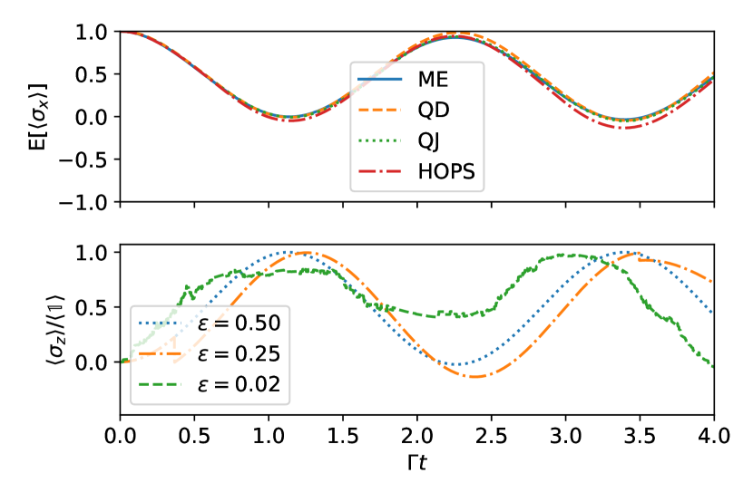
where zero mean complex noises satisfy the Ito rules $\textrm{d}Z_{\pm}\textrm{d}Z_{\pm}^{*}=\gamma_{\pm}(t)\textrm{d}t$ and $\textrm{d}Z_{\pm}\textrm{d}Z_{\pm}=\textrm{d}Z_{\mp}\textrm{d}Z_{\pm}^{*}=0$. We consider the following parameters in all of the numerical examples $\omega/\Gamma=2$, $\omega_{c}/\Gamma=5.5$, $\Omega/\Gamma=0.5$, $g=0.8$ and we plot all dynamical quantities as a function of the dimensionless time $\Gamma t$. The decay rate $\gamma(t)$ is temporarily negative when $\frac{1}{2}<\Gamma t<3/2$ for these parameter values. Figure 2 shows a good agreement between the master equation solution and its unravelings. However, we also solved the dynamics exactly using the HOPS approach to NMQSD Suess et al. (2014); Hartmann and Strunz (2017). The small disagreement shows that the approximations leading to the master equation (Example: Driven dissipative two level atom.—) are not fully consistent with the chosen parameters. Therefore, a word of caution is in place here; within the master equation approach, the quality of the obtained equation is extremely hard to assess⁵⁵5HOPS with hierarchy order 1 corresponds closely to the level of approximation we make when using- and unraveling the master quation with respect to exact dynamics. In Fig. 2 we have truncated the hierarchy after 8 levels.. In the bottom panel, we also show examples of single trajectories with LNMQJ for different values of $\epsilon$. The purpose is to demonstrate the agreement of the ensemble averages with the master equation solution – and that with our new methodological results, even driven systems can be very easily handled with the jump method whenever a reliable master equation is available.

We have provided a connection between quantum state diffusion and quantum jumps in the non-Markovian regime. As a by product of these investigations we introduced a linear version of the non-Markovian quantum jumps method and a new type of unraveling which we call non-Markovian quantum diffusion. We combined the non-Markovian quantum jumps and non-Markovian quantum diffusion with kernel smoothing techniques thus extending the applicability of these methods dramatically. Moreover, we also demonstrated the power of our approach with the paradigmatic amplitude damped driven two-level atom model. As an outlook, in addition of applying the methods for various state-of-the art complex driven open quantum systems, it would be interesting to investigate, e.g., what role the stochastic entropy term in non-Markovian quantum diffusion plays in quantum stochastic thermodynamics.

References

- Bloch et al. (2008) I. Bloch, J. Dalibard, and W. Zwerger, Rev. Mod. Phys. 80, 885 (2008).
- Gutiérrez et al. (2017) R. Gutiérrez, C. Simonelli, M. Archimi, F. Castellucci, E. Arimondo, D. Ciampini, M. Marcuzzi, I. Lesanovsky, and O. Morsch, Phys. Rev. A 96, 041602 (2017).
- Barreiro et al. (2011) J. T. Barreiro, M. Müller, P. Schindler, D. Nigg, T. Monz, M. Chwalla, M. Hennrich, C. F. Roos, P. Zoller, and R. Blatt, Nature 470, 486 EP (2011), article.
- Müller et al. (2011) M. Müller, K. Hammerer, Y. L. Zhou, C. F. Roos, and P. Zoller, New Journal of Physics 13, 085007 (2011).
- Harrington et al. (2019) P. M. Harrington, D. Tan, M. Naghiloo, and K. W. Murch, Phys. Rev. Lett. 123, 020502 (2019).
- Engel et al. (2007) G. S. Engel, T. R. Calhoun, E. L. Read, T.-K. Ahn, T. Mancal, Y.-C. Cheng, R. E. Blankenship, and G. R. Fleming, Nature 446, 782 EP (2007).
- Lee et al. (2007) H. Lee, Y.-C. Cheng, and G. R. Fleming, Science 316, 1462 (2007), https://science.sciencemag.org/content/316/5830/1462.full.pdf .
- (8) T. Brixner, R. Hildner, J. Köhler, C. Lambert, and F. Würthner, Advanced Energy Materials 7, 1700236, https://onlinelibrary.wiley.com/doi/pdf/10.1002/aenm.201700236 .
- Diósi et al. (1998) L. Diósi, N. Gisin, and W. T. Strunz, Phys. Rev. A 58, 1699 (1998).
- Strunz et al. (1999) W. T. Strunz, L. Diósi, and N. Gisin, Phys. Rev. Lett. 82, 1801 (1999).
- Yu et al. (1999) T. Yu, L. Diósi, N. Gisin, and W. T. Strunz, Phys. Rev. A 60, 91 (1999).
- Suess et al. (2014) D. Suess, A. Eisfeld, and W. T. Strunz, Phys. Rev. Lett. 113, 150403 (2014).
- Hartmann and Strunz (2017) R. Hartmann and W. T. Strunz, Journal of Chemical Theory and Computation 13, 5834 (2017).
- Roden et al. (2009) J. Roden, A. Eisfeld, W. Wolff, and W. T. Strunz, Phys. Rev. Lett. 103, 058301 (2009).
- Ritschel et al. (2011) G. Ritschel, J. Roden, W. T. Strunz, A. Aspuru-Guzik, and A. Eisfeld, The Journal of Physical Chemistry Letters 2, 2912 (2011).
- Abramavicius and Abramavicius (2014) V. Abramavicius and D. Abramavicius, The Journal of Chemical Physics 140, 065103 (2014), https://doi.org/10.1063/1.4863968 .
- Gao and Eisfeld (2019) X. Gao and A. Eisfeld, The Journal of Chemical Physics 150, 234115 (2019), https://doi.org/10.1063/1.5095578 .
- Zhong and Zhao (2013) X. Zhong and Y. Zhao, The Journal of Chemical Physics 138, 014111 (2013), https://doi.org/10.1063/1.4773319 .
- Breuer et al. (2002) H. Breuer, F. Petruccione, and S. Petruccione, The Theory of Open Quantum Systems (Oxford University Press, 2002).
- Piilo et al. (2008) J. Piilo, S. Maniscalco, K. Härkönen, and K.-A. Suominen, Phys. Rev. Lett. 100, 180402 (2008).
- Piilo et al. (2009) J. Piilo, K. Härkönen, S. Maniscalco, and K.-A. Suominen, Phys. Rev. A 79, 062112 (2009).
- Härkönen (2010) K. Härkönen, Journal of Physics A: Mathematical and Theoretical 43, 065302 (2010).
- Ai et al. (2014) Q. Ai, Y.-J. Fan, B.-Y. Jin, and Y.-C. Cheng, New Journal of Physics 16, 053033 (2014).
- Tao et al. (2016) M.-J. Tao, Q. Ai, F.-G. Deng, and Y.-C. Cheng, Scientific Reports 6, 27535 EP (2016), article.
- Rebentrost et al. (2009) P. Rebentrost, R. Chakraborty, and A. Aspuru-Guzik, The Journal of Chemical Physics 131, 184102 (2009), https://doi.org/10.1063/1.3259838 .
- Oh et al. (2019) S. A. Oh, D. F. Coker, and D. A. W. Hutchinson, The Journal of Chemical Physics 150, 085102 (2019), https://doi.org/10.1063/1.5048058 .
- Renaud and Grozema (2015) N. Renaud and F. C. Grozema, The Journal of Physical Chemistry Letters 6, 360 (2015).
- Breuer and Petruccione (1995) H.-P. Breuer and F. Petruccione, Phys. Rev. Lett. 74, 3788 (1995).
- Ghosh (2017) S. Ghosh, Kernel Smoothing: Principles, Methods and Applications (Wiley, 2017).
- Chruscinski and Jamiolkowski (2004) D. Chruscinski and A. Jamiolkowski, Geometric Phases in Classical and Quantum Mechanics, Progress in Mathematical Physics (Birkhäuser Boston, 2004).
- Note (1) Supplementary Material.
- Link and Strunz (2017) V. Link and W. T. Strunz, Phys. Rev. Lett. 119, 180401 (2017).
- Risken (2012) H. Risken, The Fokker-Planck Equation: Methods of Solution and Applications, Springer Series in Synergetics (Springer Berlin Heidelberg, 2012).
- Gardiner (2009) C. Gardiner, Stochastic Methods: A Handbook for the Natural and Social Sciences, Springer Series in Synergetics (Springer Berlin Heidelberg, 2009).
- Note (2) We demand that at time all of the decay rates have to be non-negative.
- Note (3) , when .
- Note (4) For the computation we use the results of Note (1) to compute the determinant, to expand the probability density, to expand a rational polynomial and choose with .
- Pellegrini and Petruccione (2009) C. Pellegrini and F. Petruccione, Journal of Mathematical Physics 50, 122101 (2009), https://doi.org/10.1063/1.3263941 .
- Seifert (2005) U. Seifert, Phys. Rev. Lett. 95, 040602 (2005).
- Gorini et al. (1976) V. Gorini, A. Kossakowski, and E. C. G. Sudarshan, Journal of Mathematical Physics 17, 821 (1976).
- Lindblad (1976) G. Lindblad, Commun. Math. Phys. 48, 119 (1976).
- Note (5) HOPS with hierarchy order 1 corresponds closely to the level of approximation we make when using- and unraveling the master quation with respect to exact dynamics. In Fig. 2 we have truncated the hierarchy after 8 levels.