Diffusion Methods for Generating Transition Paths ^††thanks: This work is supported in part by National Science Foundation via award NSF DMS-2012286 and DMS-2309378.

In reverse SDE denoising, we use a neural network to parameterize the time-dependent score function as $s_{\theta}(x,t)$. Since the reverse SDE involves a time-dependent score function, the loss function is obtained by taking a time average of the distance between the true score and $s_{\theta}$. Discretizing the SDE with time steps $0=t_{0}<t_{1}<...<t_{N}=T$, we get the following loss function:

Using the step size $h_{t_{i}}=t_{i}-t_{i-1}$ is a natural choice for weighting, although it is possible to use different weights. The loss function can be expressed as an expectation over the joint probability of $x_{t_{i}},x_{0}$ as [Vin11]

We can calculate $\nabla\log p_{t_{i}}(x_{t_{i}}\mid x_{0})$ based on the forward process (in the case of Ornstein-Uhlenbeck, $p_{t_{i}}(\cdot\mid x_{0})$ is a Gaussian centered at $x_{0}e^{-\beta t}$). Remarkably, this depends only on $s_{\theta}$, $t$, and the choice of forward SDE. A similar loss function is used for NCSM with a different noise-adding procedure. The training procedure follows from the above expression for the loss.

Once we have learned the time-dependent score, we can use it to sample from the original distribution using the reverse SDE. Substituting our parameterized score function $s_{\theta}$ into (2), we get an approximation of the reverse process,

We want to evaluate $s_{\theta}$ at the times at which it was trained, so we discretize the SDE from equation (2) using the sequence of times $0=\tilde{t}_{0}\leq\tilde{t}_{1}\leq...\leq\tilde{t}_{N}=T$, where $\tilde{t}_{k}=T-t_{N-k}$. In forward time (flowing from 0 to T), this discretization gives

We solve for $x_{t}$ using Itô’s formula to retain the continuous dynamics of the first term. Let $\tilde{z}_{t}=e^{-\beta t}\tilde{x}_{t}$ and $\eta_{k}$ be a standard Gaussian random variable, then

After solving for $\tilde{z}_{\tilde{t}_{k}}$, we can get an explicit expression for $\tilde{x}_{\tilde{t}_{k}}$, which is known as the exponential integrator scheme [ZC22].

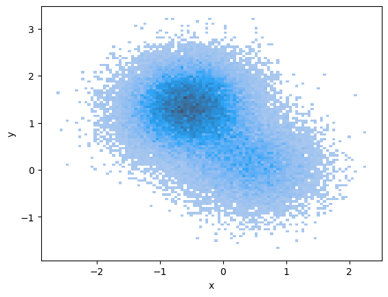
where $\eta_{k}\sim N(0,I_{d})$. We denote the distribution of $x_{t_{k}}$ as $q_{t_{k}}$. According to the literature [CLL23], using an exponentially decaying step size for the discretization points provides strong theoretical guarantees for the distance between $q_{t_{N}}$ and the true data distribution, which we will explore further in Section 4.3. For the forward process, this means that $\frac{t_{k}-t_{k-1}}{t_{k+1}-t_{k}}=M$. It is important to choose $t_{min},M$, and $N$ carefully, as they significantly affect the performance. More details about our implementation can be found in Section 5. Having estimated the score function, we can generate samples from a distribution that is close to $p_{data}$ by setting $\tilde{x}_{0}\sim p_{T}\approx N(0,\frac{1}{2\beta}I)$, then repeatedly applying (9) at the discretization points. A visualization of the distribution of $\tilde{x}$ at different $\tilde{t}_{k}$ values under this procedure is shown in Figure 1.

Transitions between metastable states are crucial to understanding behavior in many chemical systems. Metastable states exist in potential energy basins and so transitions will often occur on a longer time scale than the random fluctuations within the system. Due to their infrequency, it is challenging to effectively describe these transitions. In the study of transition paths, it is often useful to model the governing system as an SDE. In this section, we will look at the overdamped Langevin equation, given by

where $V(x)$ is the potential of the system and $W_{t}$ is d-dimensional Brownian motion. Let $\mathcal{F}_{t}=\sigma({X_{s},0\leq s\leq t})$ be the filtration generated by $X_{t}$. In chemical applications, $B^{-1}$ is the temperature times the Boltzmann constant. For reasonable $V$, the invariant probability distribution exists and is given by

We can see an example of samples generated from the invariant distribution when $V$ is the Müller potential in the above figure.

Consider two metastable states represented by closed regions $A,B\subset\mathbb{R}^{n}$. Their respective boundaries are $\partial A,\partial B$. The paths that go from the boundary of $A$ to the boundary of $B$ without returning to $A$ are called transition paths [EVE10]. This means that a realization $\{X_{s}\}_{s=0}^{T}$ is a transition path if $X_{0}\in\partial A,X_{T}\in\partial B$, and $X_{s}\notin A\cup B,\ \forall\ s\in(0,T)$. The distribution of transition paths is the target distribution of the generative procedure in our paper. A similar problem involves trajectories with a fixed time interval and is known as a bridge process. Much of the analysis in this paper can be extended to the fixed time case by removing the conditioning on path time during training and generation.

An important function for the study of transition paths is the committor function, which is defined by the following boundary value problem [EVE10], [LN15]

where $q(x)$ is the committor and $L^{P}$ is the generator for (10), defined as $L^{P}f=B^{-1}\Delta f-\nabla V\nabla f$.

We will now examine the distribution of transition paths as in [LN15]. Consider stopping times of the process $X_{t}$ with respect to $\mathcal{F}_{t}$:

Let $E$ be the event that $\tau^{(X)}_{B}<\tau^{(X)}_{A}$. We are only looking at choices of $V(x)$ such that $P(\tau^{(X)}_{A}<\infty)=1$ and $P(\tau^{(X)}_{B}<\infty)=1$. It follows from Itô’s formula that $q(x)=P(E\mid X_{0}=x)$ is a solution to (12). Thus, the committor gives the probability that a path starting from a particular point reaches region $B$ before region $A$.

Consider the process $Z_{t}=X_{t\wedge\tau_{A}\wedge\tau_{B}}$, the corresponding measure $\mathbb{P}_{x}$, and the stopping times $\tau_{A}^{(Z)},\tau_{B}^{(Z)}$. Since the paths we are generating terminate after reaching $B$, we will work with the $Z$ process, though it is possible to use the original $X$ process as well. We define $E^{*}$ as the event that $\tau_{B}^{(Z)}<\infty$. The function defined as $q(x)=P(E^{*}\mid Z_{0}=x)$ is equivalent to the committor for the $X$ process. We are interested in paths drawn from the measure $\mathbb{Q}_{x}=\mathbb{P}_{x}(\cdot\mid E^{*})$ on transition paths. The Radon-Nikodym derivative is given by

Suppose that we have a path $\{Z_{s}\}_{s=0}^{\infty}$ starting at $x$ and ending in $B$. Eq. (15) states that the relative likelihood of $\{Z_{s}\}$ under $\mathbb{Q}_{x}$ compared to $\mathbb{P}_{x}$ increases as $q(x)$ decreases. This follows our intuition, since as $q(x)$ decreases, a higher proportion of paths starting from $x$ from the original measure will end in $A$ rather than $B$.

Using Doob’s h-Transform [Day92], we have that

and the law of $Y_{t}$ given by the SDE

is equivalent to the law of transition paths. Thus, conditioning on transition paths is equivalent to adding a drift term to (10).

In this section, we introduce chain reverse SDE denoising, which learns the gradient for each point in the path separately by conditioning on the previous point. Specifically, we will use $\frac{\partial}{\partial x_{n}}\log p_{t}(x(t))$ to represent the component of score function which corresponds to $x_{n}$ and $s^{*}(x(t),t)^{(n)}$ as the corresponding neural network approximation. Unlike in the next section, here we are approximating the joint probability of the entire path (that is, $s^{*}_{\theta}(x,t)\approx p_{t}(x(t))$) and split it into a product of conditional distributions involving neighboring points as described in Figure 2. This is similar to the approach used in [HDBDT21], but without fixing time. Our new loss function significantly reduces the dimension of the neural network optimization problem:

where $x_{j}$ now denotes the $j$th point in the path. This is a slight change in notation from the previous section, where the subscript was the time in the generation process. The time flow of generation is now represented by $x(t)$. We can take advantage of the Markov property of transition paths to get a simplified expression for the sub-score for interior points,

It follows that we need two networks, $s_{\theta_{1}}(x_{n}(t),x_{n-1}(t),n,t,T^{*})$ and $s_{\theta_{2}}(x_{n}(t),x_{n+1}(t),n,t,T^{*})$. The first to approximate $\frac{\partial}{\partial x_{n}}\log p_{t}(x_{n}\mid x_{n-1},T^{*})$ and the second for $\frac{\partial}{\partial x_{n}}\log p_{t}(x_{n+1}\mid x_{n},T^{*})$. The first and last points of the path require slightly different treatment. From the same decomposition of the joint distribution, we have that

Then, the entire description of the sub-score functions is given by

where $s_{\theta_{3}}(x_{1},t,T^{*})$ is a third network to learn the distribution of initial points. As outlined in Section 2.2, we use a discretized version of the reverse SDE to generate transition paths.

While the previous approach can generate paths well, there are drawbacks. It requires learning $O(2m)$ score functions since the score for a single point is affected by its index along the path. There is a large degree of correlation for parts of the path that are close together, but it is still not an easy computational task. Additionally, all points are updated simultaneously during generation, so the samples will start in a lower data density region. This motivates using a midpoint approach, which is outlined in Figure 3.

We train a score model that depends on both endpoints to learn the distribution of the point equidistant in time to each. This corresponds to the following decomposition of the joint density. Let us say that there are $2^{k}+1$ points in each path. We start with the case in which the path is represented by a discrete Markov process $x=\{x_{j}\}_{j=1}^{2^{k}+1}$.

Based on this, we can parameterize the score function by

where $n_{s}=\frac{n_{1}+n_{2}}{2},n_{d}=n_{2}-n_{1}$. It is worth mentioning that without further knowledge of the transition path process, we would need to include $n_{1}$ as a parameter for $s_{\theta}$. However, we can see from (16) that transition paths are a time-homogeneous process, which allows this simplification. Then,

where $p^{*}$ is the transition kernel for transition paths and $f,g$ are general functions designed to show the parameter dependence of $p(x_{n^{*}}\mid x_{n_{1}},x_{n_{2}})$. The training stage is similar to that described in the previous section. For an interior point $x_{i}$, the corresponding score matching term is $s_{\theta}(x_{i},x_{i-f(i)},x_{i+f(i)},\frac{2i_{d}}{m}T^{*},t)$. For the endpoints, we have $s_{\theta_{2}}(x_{0}\mid T^{*})$ and $s_{\theta_{3}}(x_{2_{k}}\mid x_{0},T^{*})$. It is algorithmically easier to use $2^{k}+1$ discretization points for the paths, but we can generalize to $k$ points. Starting with the same approach as before, we will eventually end up with a term that can not be split by a midpoint if we want the correct number of points. Specifically, this occurs when we want to generate $n$ interior points for some even $n$. In this case, we can use

where $m^{*}=\frac{m_{1}+m_{2}+1}{2}$ or $\frac{m_{1}+m_{2}-1}{2}$. The score function will require an additional time parameter now that the midpoint is not exactly in between the endpoints. A natural choice is to use

where

A similar adaptation can be made when the points along the path are not evenly spaced. It remains to learn $P(T^{*})$, which is a simple, one-dimensional problem. We can then use times drawn from the learned distribution as the seed for generating paths.

We can extend the result from Lemma (4.1) to the continuous case. Consider a stochastic process $x(t)$ as in (1) and arbitrary times $t_{1},...,t_{n}$.

The proof follows by the same induction as in the previous case, since the Markov property still holds. This technique can be extended to problems similar to transition path generation, such as other types of conditional trajectories. It is also possible to apply the approach of non-simultaneous generation to the chain method that we described in the previous section.

We seek to obtain a convergence guarantee for generating paths from the reverse SDE using the approach outlined in Section 2.2. There has been previous work on convergence guarantees for general data distributions by [LLT23], [CLL23], [DB22], [CCL⁺22]. In particular, we can make guarantees for the KL divergence or TV distance between $p_{data}$ and the distribution of generated samples given an $L_{2}$ error bound on the score estimation. Recent results [BDBDD23] show that a bound with linear $d$-dependence is possible for the number of discretization steps required to achieve $\mathrm{KL}(p_{data}||q_{t_{N}})=\tilde{O}(\epsilon_{0}^{2})$.

With these assumptions on the accuracy of the score network and the second moment of $p_{data}$, we can establish bounds for the KL-divergence between $p_{data}$ and $q_{t_{N}}$. Using the exponential integrator scheme from Section 2.2, the following theorem from [BDBDD23] holds:

It is important to keep in mind that the KL-divergence between $p_{data}$ and $q_{t_{N}}$ does not entirely reflect the quality of the generated samples. In a practical setting, there also must be sufficient differences between the initial samples and the output. Otherwise, the model is performing the trivial task of generating data that is the same or very similar to the input data.

To exhibit the effectiveness of our algorithms, we look at the overdamped Langevin equation from (10) and choose $V$ as the two-welled Müller potential in $\mathbb{R}^{2}$ defined by

We used the following parameters, as used in [KLY19] [LLR19]

We define regions A and B as circles with a radius of 0.1 centered around the minima at (0.62, 0.03) and (-0.56, 1.44) respectively. This creates a landscape with two major wells at A and B, a smaller minimum between them, and a potential that quickly goes to infinity outside the region $\Omega:=[-1.5,1.5]\times[-0.5,2]$. We used $B^{-1}=10\sqrt{2}$ for this experiment, which is considered a moderate temperature.

For each of the score functions learned, we used a network architecture consisting of 6 fully connected layers with 20, 400, 400, 200, 20, and 2 neurons, excluding the input layer. The input size of the first layer was 7 (2 data points, $n,T^{*}$ and $t$) for the chain method and 8 for the midpoint method (3 data points, $T^{*}$ and $t$). We used a hyperbolic tangent (tanh) for the first layer and leaky ReLU for the rest of the layers. The weights were initialized using the Xavier uniform initialization method. All models were trained for 200 epochs with an initial learning rate of 0.015 and a batch size of 600. For longer paths, we used a smaller batch size and learning rate because of memory limitations. The training set was about 20,000 paths, so this example is in the data-rich regime. All noise levels were trained for every batch. We used the (9) to discretize the reverse process. We found that $t_{min}=0.005$ and $T=7$ with 100 discretization points gave strong empirical results. For numerical reasons, we used a maximum step size of 1. In particular, this restriction prevents the initial step from being disproportionately large, which can lead to overshooting.

The paths generated using either method (sample shown in Figure 4) closely resemble the training paths. To evaluate the generated samples numerically, we can calculate the relative entropy of the generated paths compared to the training paths or the out-of-sample paths (Tables 5a, 5b). We converted collections of paths into distributions using the scipy gaussian_kde function.

We can also test the quality of our samples by looking at statistics of the generated paths. For example, we can look at the distribution of points on the path. From transition path theory [LN15], we know that $p^{*}(x)\propto p(x)q(x)(1-q(x))$, where $p$ is the original probability density of the system, $p^{*}$ is the density of points along transition paths, and $q$ is the committor. This gives a 2-dimensional distribution as opposed to a $2m$ dimensional one since each of the path points is treated independently. Here, the three relevant distributions are the training, output, and ground truth distributions.

We include the average absolute difference between the three relevant distributions at 2500 grid points in Tables 6a, 6b.

The chain method slightly outperforms the midpoint method according to this metric. Qualitatively, the paths generated using the two methods look similar. There is a strong correlation between the error and the training time, but a limited correlation with the size of the training dataset after reaching a certain size. This is promising for potential applications, as the data requirements are not immediately prohibitive.

The strong dependence on training time, which is shown in Figure 6, supports the notion that the numerical results of this paper could be improved with longer training or a larger model. We further explore performance in the data-scarce case in the following section.

For our second numerical experiment, we generate transitions between stable conformers of Alanine dipeptide. The transition pathways [JW06] and free-energy profile [VV10] of Alanine dipeptide have been studied in the molecular dynamics literature and are shown in Figure 7. This system is commonly used to model dihedral angles in proteins. We use the dihedral angles, $\phi$ and $\psi$ (shifted for visualization purposes), as collective variables.

The two stable states that we consider are the lower density state around $\psi=0.6\text{ rad},\phi=0.9\text{ rad}$ (minimum A), and the higher density state around $\psi=2.7\text{ rad},\phi=-1.4\text{ rad}$ (minimum B). The paths are less regular than with Müller potential because the reactive paths "jump" from values close to $\pi$ and $-\pi$. We use 22 reactive trajectories as training data for the score network. The data include 21 samples that follow reactive pathway 1 and one sample that follows reactive pathway 2. We use the same network architecture as used for the midpoint approach in the previous section. We train the model for 2000 epochs with an initial learning rate of 0.0015.

Because the data are angles, the problem moves from $\mathbb{R}$ to the surface of a torus. We wrap around points outside of the interval $[-\pi,\pi]$ during the generation process to adjust for the new topology. This approach was more effective than encoding periodicity into the neural network. For this problem, the drift term for the forward process, $-\frac{1}{2}x$, is no longer continuous, though this did not cause numerical issues. It may be useful to use the more well-behaved process $d\Omega_{t}=\sin(-\Omega_{t})dt+\sqrt{2}dW_{t}$ applied to problems with this geometry.

We can generate paths across both reactive channels. In some trials, paths are generated that follow neither channel, instead going straight from the bottom left basin to minimum A. This occurred with similar frequency to paths across RP2. It is more challenging to determine the quality of the generated paths when there is minimal initial data, but it is encouraging that the qualitative shape of the paths is similar (Figure 8). Specifically, the trajectories tend to stay around the minima for a long time, and the transition time between them is short. For this experiment, the paths generated using the midpoint method were qualitatively closer to the original distribution. In particular, disproportionately large jumps between adjacent points occurred more frequently using the chain method, though both methods were able to generate representative paths.

References

- [BCDG02] Peter G Bolhuis, David Chandler, Christoph Dellago, and Phillip L Geissler. Transition path sampling: Throwing ropes over rough mountain passes, in the dark. Annual review of physical chemistry, 53(1):291–318, 2002.
- [BDBDD23] Joe Benton, Valentin De Bortoli, Arnaud Doucet, and George Deligiannidis. Linear Convergence Bounds for Diffusion Models via Stochastic Localization. arXiv preprint arXiv:2308.03686, 2023.
- [CCL+22] Sitan Chen, Sinho Chewi, Jerry Li, Yuanzhi Li, Adil Salim, and Anru R Zhang. Sampling is as easy as learning the score: theory for diffusion models with minimal data assumptions. arXiv preprint arXiv:2209.11215, 2022.
- [CGR19] Frédéric Cérou, Arnaud Guyader, and Mathias Rousset. Adaptive multilevel splitting: Historical perspective and recent results. Chaos: An Interdisciplinary Journal of Nonlinear Science, 29(4), 2019.
- [CHIS23] Florinel-Alin Croitoru, Vlad Hondru, Radu Tudor Ionescu, and Mubarak Shah. Diffusion models in vision: A survey. IEEE Transactions on Pattern Analysis and Machine Intelligence, 2023.
- [CLL23] Hongrui Chen, Holden Lee, and Jianfeng Lu. Improved analysis of score-based generative modeling: User-friendly bounds under minimal smoothness assumptions. In International Conference on Machine Learning, pages 4735–4763. PMLR, 2023.
- [Day92] Martin V Day. Conditional exits for small noise diffusions with characteristic boundary. The Annals of Probability, pages 1385–1419, 1992.
- [DB22] Valentin De Bortoli. Convergence of denoising diffusion models under the manifold hypothesis. arXiv preprint arXiv:2208.05314, 2022.
- [EVE10] Weinan E and Eric Vanden-Eijnden. Transition-path theory and path-finding algorithms for the study of rare events. Annual review of physical chemistry, 61:391–420, 2010.
- [FE04] Anton K Faradjian and Ron Elber. Computing time scales from reaction coordinates by milestoning. The Journal of chemical physics, 120(23):10880–10889, 2004.
- [Fle77] Wendell H Fleming. Exit probabilities and optimal stochastic control. Applied Mathematics and Optimization, 4:329–346, 1977.
- [HD05] Aapo Hyvärinen and Peter Dayan. Estimation of non-normalized statistical models by score matching. Journal of Machine Learning Research, 6(4), 2005.
- [HDBDT21] Jeremy Heng, Valentin De Bortoli, Arnaud Doucet, and James Thornton. Simulating diffusion bridges with score matching. arXiv preprint arXiv:2111.07243, 2021.
- [HJA20] Jonathan Ho, Ajay Jain, and Pieter Abbeel. Denoising diffusion probabilistic models. Advances in neural information processing systems, 33:6840–6851, 2020.
- [JW06] Hyunbum Jang and Thomas B Woolf. Multiple pathways in conformational transitions of the alanine dipeptide: an application of dynamic importance sampling. Journal of computational chemistry, 27(11):1136–1141, 2006.
- [KLY19] Yuehaw Khoo, Jianfeng Lu, and Lexing Ying. Solving for high-dimensional committor functions using artificial neural networks. Research in the Mathematical Sciences, 6:1–13, 2019.
- [LLR19] Qianxiao Li, Bo Lin, and Weiqing Ren. Computing committor functions for the study of rare events using deep learning. The Journal of Chemical Physics, 151(5), 2019.
- [LLT23] Holden Lee, Jianfeng Lu, and Yixin Tan. Convergence of score-based generative modeling for general data distributions. In International Conference on Algorithmic Learning Theory, pages 946–985. PMLR, 2023.
- [LN15] Jianfeng Lu and James Nolen. Reactive trajectories and the transition path process. Probability Theory and Related Fields, 161(1-2):195–244, 2015.
- [LRS+23] Tony Lelièvre, Geneviève Robin, Innas Sekkat, Gabriel Stoltz, and Gabriel Victorino Cardoso. Generative methods for sampling transition paths in molecular dynamics. ESAIM: Proceedings and Surveys, 73:238–256, 2023.
- [PS10] F Pinski and A Stuart. Transition paths in molecules: gradient descent in pathspace. J. Chem. Phys, 132:184104, 2010.
- [SE19] Yang Song and Stefano Ermon. Generative modeling by estimating gradients of the data distribution. Advances in neural information processing systems, 32, 2019.
- [SSDK+20] Yang Song, Jascha Sohl-Dickstein, Diederik P Kingma, Abhishek Kumar, Stefano Ermon, and Ben Poole. Score-based generative modeling through stochastic differential equations. arXiv preprint arXiv:2011.13456, 2020.
- [Vin11] Pascal Vincent. A connection between score matching and denoising autoencoders. Neural computation, 23(7):1661–1674, 2011.
- [VV10] Jiri Vymetal and Jiri Vondrasek. Metadynamics As a Tool for Mapping the Conformational and Free-Energy Space of Peptides: The Alanine Dipeptide Case Study. The Journal of Physical Chemistry B, 114(16):5632–5642, 2010.
- [ZC22] Qinsheng Zhang and Yongxin Chen. Fast sampling of diffusion models with exponential integrator. arXiv preprint arXiv:2204.13902, 2022.