Super-Kamiokande Collaboration
Diffuse Supernova Neutrino Background Search at Super-Kamiokande
Abstract
A new search for the diffuse supernova neutrino background (DSNB) flux has been conducted at Super-Kamiokande (SK), with a -ktonday exposure from its fourth operational phase IV. The new analysis improves on the existing background reduction techniques and systematic uncertainties and takes advantage of an improved neutron tagging algorithm to lower the energy threshold compared to the previous phases of SK. This allows for setting the world’s most stringent upper limit on the extraterrestrial flux, for neutrino energies below 31.3 MeV. The SK-IV results are combined with the ones from the first three phases of SK to perform a joint analysis using ktondays of data. This analysis has the world’s best sensitivity to the DSNB flux, comparable to the predictions from various models. For neutrino energies larger than 17.3 MeV, the new combined C.L. upper limits on the DSNB flux lie around cm-2, strongly disfavoring the most optimistic predictions. Finally, potentialities of the gadolinium phase of SK and the future Hyper-Kamiokande experiment are discussed.
I Introduction
I.1 Diffuse supernova neutrino background
Core-collapse supernovae (CCSNe) are among the most cataclysmic phenomena in the Universe and are essential elements of dynamics of the cosmos. Their underlying mechanism is however still poorly understood, as characterizing it would require intricate knowledge of the core of the collapsing star. Information about this core could be accessed by detecting neutrinos emitted by supernova bursts, whose luminosity and energy spectra closely track the different steps of the CCSN mechanism in a neutrino-heating scenario (see Refs. Fukugita et al. (1994); Kotake et al. (2006); Nakazato et al. (2013), for example). Existing neutrino experiments, however, are mostly sensitive to supernova bursts occurring in our galaxy and its immediate surroundings, that are extremely rare (a few times per century in our galaxy Tammann et al. (1994); Diehl et al. (2006)). Learning about the aggregate properties of supernovae in the Universe hence requires observing the accumulation of neutrinos from all distant supernovae. The integrated flux of these neutrinos forms the diffuse supernova neutrino background, or DSNB (DSNB neutrinos are also referred to as supernova relic neutrinos (SRNs) in various publications).
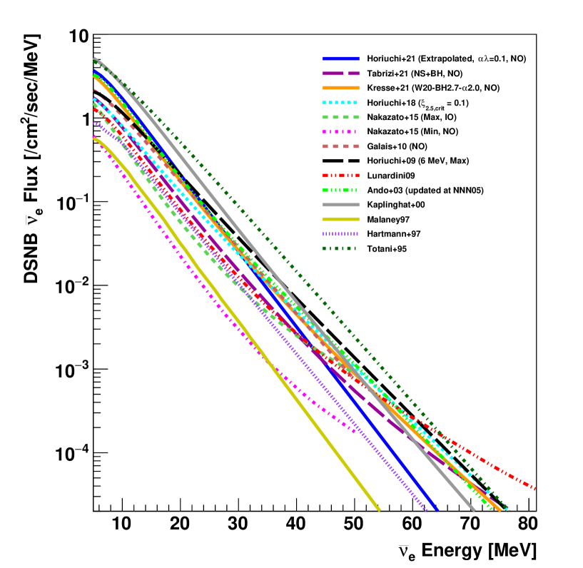
The DSNB is composed of neutrinos of all flavors whose energies have been redshifted when propagating to Earth. Its spectrum therefore contains unique information not only on the supernova neutrino emission process but also on the star formation and Universe expansion history. Spectra predicted from various models are shown in Fig. 1. Their overall normalization is mostly determined by the supernova rate, related to the cosmic star formation rate. While this redshift-dependent rate also impacts the DSNB spectral shape, the latter is mainly affected by the effective energies of supernova neutrinos.
Other factors shaping the DSNB spectrum include the neutrino mass ordering, the initial mass function of progenitors, the equation-of-state of neutron stars, the fraction of black-hole-forming supernovae, the revival time of the shock wave, etc. Possible combinations of these factors were systematically studied in the Nakazato15 model Nakazato et al. (2015), the maximal and minimal fluxes of which are shown in the figure. The minimal prediction from this model and the Malaney97 gas infall model Malaney (1997) give the lower bounds on the DSNB flux. Conversely the Totani95 model Totani and Sato (1995) can be considered an upper bound on the expected DSNB flux, on par with the most optimistic predictions of the Kaplinghat00 model Kaplinghat et al. (2000), also shown in the figure. Between these bounds, the DSNB flux can vary over one order of magnitude and its spectral shape bears the imprint of a wide range of physical effects. Black-hole-forming supernovae notably make the DSNB spectrum harder, as can be seen with the Lunardini09 model Lunardini (2009), that assumes that of core-collapse supernovae lead to black-hole formation. Similarly, the Horiuchi18 model Horiuchi et al. (2018) incorporates a fraction of black-hole-forming supernovae determined using the stars’ compactness. Aside from accounting for black-hole formation, the Kresse21 model Kresse et al. (2021), on the other hand, uses state-of-the-art supernova simulations to model contributions from helium stars to the DSNB. Another recent study (Horiuchi21 Horiuchi et al. (2021)) discusses the impact of interactions in binary systems, such as mergers, and mass transfer, on the DSNB flux. Detecting the DSNB would hence provide valuable insights into a wide array of physical processes.
I.2 Experimental searches
While a significant fraction of DSNB neutrinos are expected to have energies lower than 10 MeV —as shown in Fig. 1—, the MeV region is hard to probe by current experiments due to overwhelming backgrounds from reactor antineutrinos, solar neutrinos, and radioactivity. Experimentally the DSNB signal has therefore been searched for at energies of MeV. At these energies, the dominant detection channel in most experiments is the inverse beta decay (IBD) of electron antineutrinos (), and contributions from subleading channels such as electron neutrino elastic scattering or charged current interactions on oxygen can be neglected. This process produces an easily identifiable positron and a neutron (Fig. 2). Here the neutron does not emit Cherenkov or scintillation light directly but its capture on a proton leads to emission of a MeV photon. In pure water, the characteristic timescale for neutron moderation and capture is of s Cokinos and Melkonian (1977). Pairing the “prompt” positron signal with the “delayed” photon emission from neutron capture is hence a key component of many analyses.

Up to now, no evidence for the DSNB signal has been confirmed and upper limits have been set by various underground experiments, such as Super-Kamiokande (SK) Malek et al. (2003); Bays et al. (2012); Zhang et al. (2015), KamLAND Gando et al. (2012); Abe et al. (2021a), SNO Aharmim et al. (2006, 2020) and Borexino Agostini et al. (2021). Note that, unlike other searches, the SNO analysis is sensitive to electron neutrinos and, due to the irreducible solar neutrino background, its effective energy threshold lies around the hep solar neutrino flux endpoint, around 19 MeV. Among all past analyses, the SK and KamLAND experiments placed the most stringent upper limits on the DSNB flux for neutrino energies above about 9 MeV while Borexino set the tightest constraints at lower energies. At SK the first DSNB search was carried out in 2003 using a -ktonday data set Malek et al. (2003). Using spectral shape fitting for signal and atmospheric neutrino backgrounds, it placed an upper limit on the DSNB flux for a wide variety of models in the 19.383.3 MeV neutrino energy range. This analysis already allowed to disfavor the most optimistic DSNB predictions, in particular the Totani95 model Totani and Sato (1995), and constrain the parameter space of the Kaplinghat00 model Kaplinghat et al. (2000). In 2012, an improved analysis was performed at SK, using a -ktonday exposure, a lower neutrino energy threshold of MeV, and new event selection cuts allowing a 50% increase in signal efficiency Bays et al. (2012). Below 17.3 MeV, large backgrounds from cosmic muon spallation and solar neutrino interactions make it extremely difficult to search for DSNB antineutrinos based on positron identification alone. A search for extragalactic antineutrinos performed at KamLAND in 2021 Abe et al. (2021a) probed neutrino energies ranging from to MeV by investigating coincident positron and neutron capture signals. While neutron identification in a liquid scintillator detector such as KamLAND is significantly easier than in pure water, KamLAND’s small fiducial volume only allowed for an exposure of ktonyear. In 2015, a new SK analysis including neutron identification led to stronger constraints down to MeV neutrino energies Zhang et al. (2015). Since the SK triggers did not allow to record the neutron capture signal until 2008, this analysis could only be performed on a small part of the SK data set, with a total livetime of ktondays. Due to this low exposure and the low neutron tagging efficiency in water, this search however yielded weaker limits than the SK-I,II,III analysis Bays et al. (2012) above 17.3 MeV.
In this study, we draw on the previous SK analyses to present two DSNB searches for antineutrino energies ranging from to MeV, with significantly improved background modeling and reduction techniques. In the to MeV range, we derive differential upper limits on the flux independently from the DSNB model, following the strategy outlined in Ref. Zhang et al. (2015) using a -ktonday data set. In the to MeV range we constrain a wide variety of DSNB models using spectral fits analogous to the ones described in Ref. Bays et al. (2012). We then combine the results of this analysis with the ones obtained in Ref. Bays et al. (2012) for the former SK phases, thus analyzing -ktondays of data. This unprecedented exposure will allow to probe the DSNB with an unmatched sensitivity.
The rest of this article proceeds as follows. First, the SK detector and the specific features of its data acquisition system are described in Section II. Then, details about modeling of the DSNB signal and the different backgrounds are given in Sections III and IV, respectively. We then describe the data reduction process in Section V. The procedures associated with the DSNB model-independent and spectral analyses are described in Sections VI and VII, respectively. Finally we discuss the current constraints on the DSNB flux and future opportunities at SK with gadolinium and Hyper-Kamiokande in Section VIII before concluding in Section IX.
II Super-Kamiokande
Super-Kamiokande is a 50-kton water Cherenkov detector located in the Kamioka mine, Japan. It is structured by a cylindrical stainless steel tank with a diameter of m and height of m and consists of two parts: an outer detector (OD) that serves as a muon veto and an inner detector (ID) where neutrino detection takes place. In order to reduce backgrounds due to radioactivity near the detector wall, most analyses consider only events reconstructed at least 2 m away from the ID wall, thus defining a 22.5-kton fiducial volume (FV). It is located 1000 m underground, that allows reduction of the cosmic ray muon flux by a factor of . In order to ensure a high-quality data taking, conditions inside SK are tightly controlled; water is constantly recirculated and purified, and the ID wall is covered with 11,129 20-inch photomultipliers (PMTs) with a -ns time resolution, corresponding to a photocathode coverage. These features allow SK to detect particles with energies ranging from a few MeV to a few TeVs. The OD includes 1,885 8-inch PMTs, facing outwards, to detect the Cherenkov light from muons. Further detailed descriptions of the SK detector and its calibration can be found in Refs. Fukuda et al. (2003); Kume et al. (1983); Abe et al. (2014a); Nakahata et al. (1999); Blaufuss et al. (2001).
SK is currently undergoing its sixth data taking phase since it started functioning in 1996. The first phase lasted days and ended for a scheduled maintenance. Due to an accident following the maintenance, which resulted in a loss of % of the ID PMTs, SK operated with a reduced photocathode coverage for days (phase II). The coverage was brought back to its nominal value for phase III, that lasted days. SK’s previous spectral analysis of the DSNB Bays et al. (2012) used data from all these three phases. Since 2008, the front-end electronics has been replaced Nishino et al. (2009) and a new trigger system that allows for neutron tagging has been set up Watanabe et al. (2009). SK operated with this new electronics during phase IV, for 2970 days, until being stopped for refurbishment work in May 2018. After the maintenance, SK operated for a short time with pure water for calibration and monitoring purposes (phase V) since January 2019, before being loaded with gadolinium (phase VI) in July 2020. This study will primarily focus on phase IV, and will present a combined analysis of the SK-I to IV data. Additionally, we will briefly discuss the opportunities offered by the gadolinium lodaded SK and by the future Hyper-Kamiokande experiments.
Data processing in SK makes use of multiple triggers, corresponding to different thresholds on the number of PMT hits found in a -ns window. In SK-I to III, all PMT hits in a 1.3-s window around the main activity peak were stored, using hardware triggers. Since SK-IV, the new data acquisition system acquires every PMT signal and a software trigger system defines events. To identify positrons from IBD processes, we use the super-high-energy (“SHE”) trigger, which requires 58 PMT hits (70 hits before September 2011) in ns. The data in a -s window around the main activity peak is collected with this trigger. This window is too short to contain the delayed neutron capture signal after IBDs. In order to identify this signal, a 500-s (s before November 2010) after trigger (“AFT”) window follows each SHE trigger that is not associated with a pre-determined OD trigger. The trigger conditions for the different periods in SK-IV are summarized in Table 1. In the rest of this paper, we will describe the analysis of hit patterns in these large SHE+AFT windows to identify the coincident production of a positron and a neutron.
The prompt positron event is reconstructed using the dedicated solar neutrino Hosaka et al. (2006); Cravens et al. (2008); Abe et al. (2011, 2016) and muon decay electron vertex and direction fitter, which is then used to reconstruct the event energy Smy (2008). For this SK phase, we follow the convention introduced in Ref. Abe et al. (2016) and subtract the 0.511 MeV electron mass from this energy to obtain the electron equivalent kinetic energy . This quantity can also be interpreted as the total reconstructed positron energy, and will be used to present the results of this study.
| SHE-threshold | AFT-window | Livetime |
|---|---|---|
| 70 hits | 350 s | 25.0 days |
| 70 hits | 500 s | 869.8 days |
| 58 hits | 500 s | 2075.3 days |
III Signal modeling
III.1 DSNB spectra and kinematics
In this analysis we consider both the DSNB models whose fluxes are shown in Fig. 1 and models where we vary specific physical parameters. For these parameterized models we compute the DSNB flux using the following formula:
| (1) |
where is the neutrino energy, is the speed of light in vacuum, is the Hubble constant, is the redshift, is the redshift-dependent supernova rate, and is the supernova neutrino emission spectrum for a given flavor . The index represents the different possible classes of supernovae —e.g. supernovae collapsing into neutron stars or black-holes— associated with specific neutrino emission spectra. The last factor accounts for the Universe expansion, with and being the matter and dark energy contributions to the energy density of the Universe, respectively. We evaluate the supernova rate using a phenomenological model described in Ref. Horiuchi et al. (2009), which extracts the redshift dependence of the cosmic star formation history by fitting observations and uses the Salpeter initial mass function Salpeter (1955) to obtain the fraction of supernova progenitors. We then consider blackbody neutrino emission spectra, where the effective temperature takes into account neutrino oscillation effects. For a given neutrino flavor the spectrum for a model with effective temperature is thus given by:
| (2) |
where is the total energy of the neutrinos emitted by the supernovae and represents the fraction of neutrinos or antineutrinos with flavor and can be roughly approximated by for a given species. The blackbody model therefore only depends on the neutrino temperatures and luminosities. In what follows, we will refer to blackbody models with a neutrino effective temperature as Horiuchi09 MeV models. Note that, due to neutrino scattering in the densest regions of the collapsing star, supernova neutrino emission is better modeled using a more sharply peaked, “pinched”, Fermi-Dirac spectrum Keil et al. (2003); however, the current exposure at SK does not allow to probe this pinching effect. In this analysis we neglect the effects of degeneracies between the pinching parameter and e.g. the neutrino temperature on the final constraints on neutrino emission spectra.
This analysis exclusively focuses on the detection of electron antineutrinos via IBD processes. In the rest of this paper, we model these processes using the Strumia-Vissani IBD calculation Strumia and Vissani (2003), that approximates the IBD cross section more precisely than the Beacom-Vogel calculation used for previous SK analyses Bays et al. (2012).
III.2 Detector simulation
SK-IV has been the longest data taking phase of the experiment, lasting about years. During this term, the PMT gain has steadily increased by about 15% over the whole SK-IV period. Additionally, since the energy scale change due to the gain change for this analysis was about 3 %, that effect was corrected in order to maintain the stability of the detector. A key ingredient of our DSNB study is therefore a simulation of antineutrino IBD processes that accounts for the evolution of the detector’s properties throughout the entire SK-IV period.
In this study we simulate IBD processes uniformly distributed in the entire inner detector, in order to account for events close to the ID wall being misreconstructed inside the fiducial volume. For each vertex we generate a set of three momentum vectors corresponding to an antineutrino, a positron, and a neutron. In a view of the wide diversity of DSNB models, we generate uniformly distributed positron energies in 190 MeV and renormalize events later to model specific spectra. This procedure will also allow to use this simulation to model backgrounds associated to other IBD processes or decays, as will be mentioned later. We then simulate detection signals using a dedicated simulation, based on GEANT3 Brun et al. (1994), that reproduces the properties of the water in SK, as well as models the PMT properties and electronic response. Detector properties such as water transparency and PMT noise are being measured daily, allowing to accurately model the time-dependent noise contamination of the positron signal. Neutron capture, however, produces a MeV ray whose light yield is below the SK trigger threshold and particularly difficult to distinguish from PMT dark noise and low energy radioactive decays. In order to develop robust neutron identification techniques we therefore collect noise samples from data using a random wide trigger, and inject them into simulation results, after the positron activity peak.
IV Background Sources
IV.1 Atmospheric neutrinos
Atmospheric neutrinos are an important background in the present DSNB searches. Below about 15 MeV, neutral-current quasielastic (NCQE) interactions, which induce nuclear ray emission Ankowski et al. (2012); Abe et al. (2014b); Wan et al. (2019); Abe et al. (2019), form the main atmospheric neutrino background. On the other hand, charged-current quasielastic (CCQE) interactions and pion production dominate at higher energies. A typical visible signature for these interactions is the Cherenkov light from electrons produced by muon and pion decays. Hence, the associated reconstructed energies will follow a Michel spectrum for reconstructed energies of about 15 to 50 MeV. Atmospheric neutrino events are simulated using the HKKM 2011 flux Honda et al. (2007, 2011); bib (Flux) as an input to the neutrino event generator NEUT 5.3.6 Hayato (2009) to model interactions. Details about the model parameters used in this analysis can be found in Ref. Abe et al. (2020). The nuclear deexcitation ’s are simulated based on the spectroscopic factors for the , , and states calculated in Ref. Ankowski et al. (2012). More detailed descriptions of the excited states can be found in Refs. Abe et al. (2014b, 2019) for the T2K NCQE measurement. One difference between our procedure and Ref. Abe et al. (2019) is treatment of the others state —a state affected by short-range correlations or with a very high excitation energy—. This state is treated as the highest excitation state () in Ref. Abe et al. (2019) while it is included in the ground state () in the present analysis as it is from the latest atmospheric neutrino analysis in SK Jiang et al. (2019). The systematic uncertainty regarding this treatment is considered in the scaling factor used in Section VI.1.
The detector simulation for atmospheric neutrino events is performed using the same GEANT3-based simulation tool as for the signal, but without corrections for the PMT gain shift on the primary event. The associated systematic error is estimated in Section VI.1 and found to be subdominant. Finally, random trigger data are overlaid on top of neutron capture signals in order to simulate background for neutron tagging, following the procedure described in Section III.2. Note that for this last step the time evolution of the detector properties is taken into account.
IV.2 Cosmic ray muon spallation
In spite of its 2700-m water-equivalent overburden, SK is still exposed to cosmic ray muons with a rate of 2 Hz. Interactions of these muons in water produce electromagnetic and hadronic showers. Spallation of oxygen nuclei induced by the muons or by secondary particles can then lead to the production of radioactive isotopes, whose decays can be misidentified as IBD events in the DSNB search window. Below about 20 MeV, the associated background is times higher than the DSNB flux predictions, making spallation reduction an essential aspect of this analysis. Since most spallation isotope decays only produce and rays, spallation backgrounds can be significantly reduced using neutron tagging. Nonetheless, accidental pairing between prompt or events and PMT hits due to dark noise or intrinsic radioactivity will allow a sizable number of spallation events to pass as IBDs. Furthermore, a few isotopes undergo a + decay that mimics the IBD signal, and thus cannot be removed using neutron tagging. Efficient spallation reduction therefore requires both dedicated spallation reduction techniques tailored to the properties of the different isotopes, and neutron tagging cuts.
Relevant spallation isotopes and their visibility in water have been studied with the FLUKA simulation Battistoni et al. (2007) in Refs. Li and Beacom (2014, 2015a, 2015b). The isotope lifetimes and the end-point energies of their decays are summarized in Fig. 3. The highest end-point is 20.6 MeV, from and . The spallation cuts used in this analysis will therefore be applied up to MeV reconstructed kinetic electron energy in order to account for energy resolution effects. Note also that the isotope half-lives range from sec to a few tens of seconds. Given the high rate of cosmic ray muons, pairing a given isotope decay with its parent process is a particularly difficult endeavour.

Isotopes that undergo decays cannot be rejected using neutron tagging and therefore need to be modeled with particular care. This is notably the case for 8He, 11Li, 16C, and 9Li. Here 11Li is particularly short-lived and therefore easy to eliminate using mild spallation cuts. Its production yield is also expected to be particularly low (around gcm2 Li and Beacom (2014)). In addition, 8He and 16C will remain subdominant due to their low production yields (around 0.23 and gcm2 Li and Beacom (2014)) and endpoint decay energies. On the other hand, 9Li has a non-negligible yield (around gcm2 Li and Beacom (2014)), a medium half-life of about sec, and decays into a pair with a branching ratio of 50.8%. The associated spectrum is shown in Fig. 4, and extends up to MeV reconstructed energy when accounting for resolution effects. The + decay of 9Li is hence similar to the IBD of a DSNB neutrino, except that the from is an electron and the neutron energy is higher than that from IBDs. Since SK does not distinguish electrons from positrons and does not allow to measure the neutron energy, we model 9Li decay using the IBD Monte-Carlo simulation, renormalizing events to reproduce the 9Li + spectrum. Finally, we estimate the total expected number of 9Li + decays in the DSNB search window by using an earlier SK measurement Zhang et al. (2016) that estimated the 9Li production rate to be . Note that the difference in neutron energies with respect to IBD processes leads to a systematic uncertainty. However, this uncertainty is taken into account when calibrating neutron tagging efficiencies, as neutrons from the calibration source have similar energies to the 9Li decay products. More details about this calibration procedure are given in Section V.4.

IV.3 Reactor neutrinos
Antineutrinos emitted from nearby nuclear reactors can undergo IBDs in SK and therefore be mistaken as the DSNB signal at low energies. We estimate the reactor antineutrino flux using the SKReact code bib (eact) developed for the SK reactor neutrino analysis. This code uses the reactor neutrino model from Ref. Baldoncini et al. (2015) based on IAEA records int (2005) to evaluate the electron antineutrino fluxes for any reactor in the world, and simulates oscillation effects. The resulting flux prediction also accounts for the time dependence of the reactor antineutrino flux due to changes in reactor activity. The expected total reactor neutrino flux at SK can thus be predicted up to MeV. The expected reactor neutrino spectrum is obtained from this predicted flux using the IBD simulation, and is shown in Fig. 5. Above 6 MeV, as can be seen in this figure, the reconstructed spectrum is primarily shaped by resolution effects. Since the reactor antineutrino spectrum has been constrained up to 12 MeV by Daya Bay An et al. (2017), possible antineutrino contributions above can be safely neglected in this study. In the 7.59.5 MeV reconstructed kinetic electron energy range, the reactor antineutrino background is about 6 times higher than the DSNB signal predicted by the Horiuchi09 6 MeV model Horiuchi et al. (2009). Reactor antineutrino backgrounds thus effectively set a lower energy threshold for the DSNB search.

IV.4 Solar neutrinos
Electron neutrinos from the Sun cause elastic interactions with electrons in SK. In the DSNB search window, the 8B and hep solar neutrino fluxes represent an important background up to 20 MeV. This background can be drastically reduced by neutron tagging, although a small fraction of electrons from solar neutrinos will be accidentally paired with background fluctuations or radioactive decays, like for the spallation backgrounds. In the absence of neutron tagging, a solar neutrino interaction can still be identified by comparing the reconstructed directions of the scattered electron to the direction of the Sun at the detection time. The angle between these two directions, called the opening angle, is expected to be close to zero for solar electron neutrinos scattering elastically. It is however smeared by reconstruction effects that need to be modeled accurately. In this study, we use the simulation designed for the latest SK-IV solar neutrino analysis Abe et al. (2016) to model solar neutrino spectra and evaluate the impact of opening angle cuts.
Finally, note that in this analysis we do not study the impact of solar antineutrino production, since the rate predicted by the Standard Model (SM) is negligible. Antineutrino production via beyond the SM processes would yield a signal that can only be distinguished from the DSNB signature by spectral shape studies. So far, only upper limits on the solar antineutrino flux have been derived at SK, notably in Ref. Abe et al. (2020).
V Data reduction
We apply reduction cuts to the data taken by the SHE trigger in SK-IV, corresponding to an exposure of ktondays. The SHE trigger efficiency is close to % over the entire analysis window. The following sections describe the four reduction steps used in this analysis: noise reduction in Section V.1, spallation reduction in Section V.2, DSNB positron candidate selection in Section V.3, and neutron tagging in Section V.4.
V.1 Search energy range and noise reduction
The lower energy threshold for this analysis is the SHE trigger threshold, which corresponds to 7.5 or 9.5 MeV depending on the observation time (see Table 1). The upper bound of the DSNB analysis window is set to MeV for the model-independent analysis and MeV for the spectral analysis.
We first select SHE-triggered events with below MeV and apply a set of cuts aimed at removing PMT noise, calibration events, radioactivity from the surrounding rock and the detector wall, and cosmic ray activity. In particular, we require candidate events to be located at least m away from the ID wall, thus defining a fiducial volume (FV) of kton. Additionally, we remove events associated with an OD trigger, or within s of another event with reconstructed electron kinetic energy larger than MeV, in order to remove electrons produced by the decay of low energy cosmic ray muons stopping in the detector. In addition, we apply fit quality cuts to eliminate noise-like events. Inside the FV these noise reduction cuts have a signal efficiency larger than as confirmed by the IBD Monte-Carlo simulation. Finally, we require all SHE events to be followed by an AFT trigger to allow for neutron tagging. Due to occasional deadtime induced by trigger software failure, this step is associated with a 94% signal efficiency. Events passing these criteria will be subsequently referred to as “DSNB candidates”.
V.2 Spallation reduction
Spallation backgrounds largely dominate over putative DSNB signals for reconstructed electron kinetic energies lower than MeV. Here, we present a set of dedicated cuts that will allow for a substantial reduction of these backgrounds, even in the absence of neutron tagging.
V.2.1 Spallation preselection
We apply two sets of preselection cuts to reduce contributions from the most energetic muons and some long-lived spallation isotopes such as 16N, with minimum harm to the signal efficiency.
First, since energetic muons could induce the production of multiple radioactive isotopes, we remove all DSNB candidates observed within 60 sec and 4.9 m from at least one other low energy event with in the 5.5-24.5 MeV range Locke et al. (2021). The 60 sec time window has been chosen to include decays of abundant and long-lived isotopes such as 16N while the 4.9-m distance cut provides optimal signal over background separation. We estimate the signal efficiency of this so-called “multiple spallation cut” using a sample of low energy events from radioactive decays at SK ( MeV), whose reconstructed vertices have been replaced by random vertices inside the ID. The cut parameters introduced above allow to remove about of the background with a signal efficiency, as can be seen in Fig. 6. Since this cut removes low energy events clustered in space and time, it also removes low energy muons that are misclassified as electrons with tens of MeV energies. These muons are not targeted by the other spallation cuts applied in this study, which assume that the prompt event is an electron or a positron. Consequently, in this study, we will apply this cut over the whole energy range for each of our analyses, including the spallation-free MeV region.

In addition to removing multiple spallation events, we locate muon-induced showers by identifying neutron captures observed less than s after muons. These neutron clusters, called “neutron clouds”, are often produced in muon-induced hadronic showers, that are the birthplaces of spallation isotopes. Neutron capture events following muons are collected separately from DSNB candidates, using a specific trigger called the Wideband Intelligent Trigger (WIT) Carminati (2011, 2015); Elnimr (2017). This trigger, in addition to setting a threshold on the number of PMT hits, applies cuts on the event quality and distance of the reconstructed vertex to the ID wall. Events triggered by WIT less than s after a given muon are considered as neutron captures if their reconstructed vertex is within m of the reconstructed muon track. If multiple neutron captures are observed after a muon event, we define a neutron cloud using the criteria from Ref. Locke et al. (2021). We then remove DSNB candidates that are found close in time and space to these neutron clouds, following the procedure introduced in Ref. Locke et al. (2021). More details about the cut criteria are given in Appendix A. To estimate the signal and background efficiencies of the neutron cloud cut, we pair muons with DSNB candidates in data, defining two samples: a “pre-sample”, including muons found up to sec before a DSNB candidate, and a “post-sample”, with muons found up to sec after a candidate. While the pre-sample contains a mixture of correlated and uncorrelated pairs, the post-sample contains only uncorrelated pairs. This sample can hence be used to both readily estimate signal efficiencies and characterize the properties of the pairs formed by each isotope decay and their parent muon in the pre-sample. An example of how to extract the distribution of the distances between spallation events and the neutron clouds of their parent muons is shown in Fig. 7. We optimize the neutron cloud cut by estimating the shape of the neutron clouds from data and maximizing the statistical significance of the signal over the spallation background. The performance of this cut is however currently limited by the weakness of the neutron capture signal and the fact that the WIT trigger has only been available only during the last 388 live days of SK-IV. While the signal efficiency is larger than % this cut only removes about % of the spallation background in this analysis. Over the 388 days of the WIT trigger livetime, however, it removes about 40% of spallation isotope decays.

Finally, it should be noted that the multiple spallation and the neutron cloud cuts described above are expected to overlap since muons associated with large hadronic showers are also likely to lead to the production of multiple isotopes. Accounting for this overlap, these preselection cuts allow to remove about 55% of the spallation background when neutron cloud data are available.
V.2.2 Searching for parent muons
Since preselection cuts remove only about half of the spallation background, a more in-depth study of the correlations between muons and DSNB candidates is necessary. In particular, in order to identify the decays of spallation isotopes, it is crucial to associate each isotope with its parent muon. Due to the long half-lives of isotopes such as 11Be and 16N, we need to investigate all possible pairings between DSNB candidates and muons observed up to 30 sec before them. This window size allows to accommodate most decay products, without processing a prohibitively high number of muons. As with neutron cloud cut optimization, we define pre- and post-samples in order to extract the observable distributions associated with spallation pairs and estimate signal efficiencies.
We define candidate muons by selecting events associated with more than 31 PMT hits (34 before May 2015) in 200 ns and depositing more than 500 in the ID. Additionally, since the SK trigger windows can contain multiple events, we also look for muons around the main activity peak in these windows. For the same reason, calibration trigger windows are also thoroughly investigated. The properties of the muon candidates, such as the charge deposited in the detector, the entry point, and the direction of the track, are then extracted using a dedicated fitter Conner (1997); Desai (2004); Bays et al. (2012). This fitter classifies muons into five categories: misfits (1.0%), single through-going muons (82.2%), stopping muons (4.9%), multiple-track muons (7.6%), and corner clippers (4.3%); the fractions of the different categories in the SK-IV data are shown in parentheses. Misfit muons with a charge lower than are removed in order to reject non-muonic high energy events. This cut does not affect removing spallation background because the track length of these low charge muons through the ID is typically less than 50 cm.
After having paired DSNB candidates with the muons selected above, we extract the following observables, related to the intrinsic properties of the muons and their correlations with DSNB candidates.
-
•
: time difference between a muon and the DSNB candidate. For spallation events, this observable reflects the half-lives of the produced isotopes.
-
•
: transverse distance of the DSNB candidate to the muon track (see Fig. 8). This observable is related to the path lengths of the secondary particles from muon showers. For well-fitted single through-going muons paired with their associated spallation isotope decays, is typically no larger than a few meters.
-
•
: longitudinal distance to the point of the muon track associated with the maximal energy deposition (see Fig. 8). The energy deposition along the muon track is determined by projecting back the light seen by each PMT to a point on the muon track, following the procedure described in Ref. Bays et al. (2012). So provides an estimate of the distance between the low energy event and the origin of the particle shower and, if the shower position is correctly identified, should also not be larger than a few meters for spallation pairs.
-
•
: total charge deposited by muons in the detector. Higher values of this observable are expected when a shower is produced. While this observable also includes contributions from minimum ionization along the muon track —and hence strongly depends on the muon track length, it provides the most robust shower predictor for poorly-fitted muons and muon bundles. Conversely, for well-fitted single through-going muons, the shower can be more accurately characterized by the observable described below.
-
•
: residual charge deposited by a muon compared to the value expected from the minimum ionization. This observable can be expressed as:
where and are the number of per centimeter expected from the minimum ionization and the track length, respectively. Here depends on detector properties, such as water transparency, that vary with time and is therefore recomputed for each run. For muons with multiple tracks, is the length of the first track. This observable allows to determine how likely a given muon is to induce a shower.

An example set of these spallation variables for single through-going muons is shown in Appendix A. The distributions associated with corner clipping muons show no evidence for spallation. Moreover, as discussed in Ref. Locke et al. (2021), spallation background events associated with corner clipping muons are expected to represent less than of the total number of spallation events. In the rest of this study, we will therefore neglect contributions from these muons to spallation backgrounds.
Showers induced by muon spallation can be extremely energetic and involve up to thousands of particles, notably neutrons and pions. Such neutrons cause nuclear reactions and possibly produce deexcitation rays, and are later captured at a timescale up to 500 s. The MeV-scale rays or particles —produced by the initial neutron, secondary nuclear reactions, or the decay product of a short-lived isotope, followed by a 2.2 MeV ray from neutron capture can mimic an IBD signature. To prevent these from leaking into the sample, we require DSNB candidates to be more than ms away from any muon. The impact of this cut on the signal efficiency is negligible. Additionally, we apply a set of cuts on and for different energy ranges, exploiting the dependence of the isotopes’ half-lives in their endpoint energies shown in Fig. 3. Detailed descriptions of these rectangular cuts are given in Appendix A. These cuts are particularly efficient above 15.5 MeV where short-lived isotopes dominate. In 15.519.5 MeV, notably, they allow to remove about 85% of the spallation background while keeping 88% of the signal events. Finally, in order to further eliminate spallation backgrounds, we use distributions of the different observables considered here to define log-likelihood ratios. First, we prepare two probability density functions (PDFs): the spallation PDF () and the random PDF (), for each variable . We isolate contributions from spallation events by subtracting the post-sample distributions from the corresponding pre-sample distributions and obtain after area normalization of these subtracted distributions. For we normalize post-sample distributions by their areas. We repeat this procedure for each category of muons. For single through-going and multiple track muons, that generate most of the spallation background, we tune the PDFs in and bins. These bins, adjusted by considering the isotopes’ typical half-lives and the distributions, account for the correlations between these observables. For each set of PDFs, we then define log-likelihood ratios as:
| (3) |
Separate likelihoods are defined for each muon category, except for corner clippers, whose contributions to spallation backgrounds are negligible as mentioned above. Note that for misfit muons only is used to calculate log-likelihood ratios, as the other observables are not reliable. An example distribution of the log-likelihood ratio is given as Fig. 33 in Appendix A. We finally determine cut conditions for each likelihood ratio, accounting for complex correlations between spallation observables, geometrical and muon reconstruction effects.
The signal efficiencies and background rejection rates of the resulting cuts are estimated using the random sample introduced in this section, as well as spallation-dominated data samples. These samples as well as our methodology to estimate the spallation cut performance are described in detail in Appendix A. Note that the estimates of the spallation remaining rate presented there are used only for cut optimization and not for the final background predictions shown in Sections VI and VII. The current cuts achieve significant improvement over the previous cuts used in Refs. Bays et al. (2012); Zhang et al. (2015), especially at low energies; for the same spallation remaining rate, the signal efficiency is increased by up to 60% for MeV, 20% for MeV, and comparable for higher energies.
V.3 DSNB positron candidate selection
In the region above 20 MeV, spallation backgrounds can be reduced to negligible levels using a series of spallation cuts while keeping most of the signal. However, significant backgrounds from atmospheric neutrino interactions and radioactive decays remain. To identify them, we define the following discriminating observables, aimed at characterizing the prompt event.
V.3.1 Incoming event cut
Radioactivity near the detector wall as well as muon spallation in the rock surrounding the detector, can lead to electrons or rays entering FV. Instead of tightening the FV cut, we consider the effective distance of each event to the ID wall Bays et al. (2012); Hosaka et al. (2006). This observable is computed by following the reconstructed direction of each event backwards from its reconstructed vertex to the ID wall, and can be interpreted as the minimal distance needed for a radioactive particle produced near the wall to travel to the event vertex, as shown in Fig. 9. The distributions for the DSNB signal and for the events selected using the cuts outlined in Section V.1 are shown in Fig. 10, for the reconstructed energy ranges corresponding to the model-independent analysis, to MeV, and the spectral analysis, to MeV. Comparing the distributions from the data and the Monte-Carlo simulation allows to estimate contributions from radioactivity near the wall, and determine a suitable cut. In this study we impose lower thresholds on ranging from to m depending on the reconstructed energy:


V.3.2 Pre- and post-activity cuts
Atmospheric neutrino interactions can produce both prompt signals from photons, electrons, or energetic heavy particles, and delayed signals from decay of muons and pions to electrons. These signals will be typically separated by a few microseconds and can therefore share the same trigger window. Depending on which particle deposits most light, unusually high activity can be noticed either before or after the main peak. For pre-activity we compute the maximal number of hits, , in a -ns time-of-flight subtracted window between s and ns before the main peak. We apply a similar procedure to post-activity, using an algorithm developed for other analyses in SK and T2K that computes the number of electrons from muon and pion decay Abe et al. (2017). The distributions for low and high energy events are shown in Fig. 11. In the analyses discussed here we require and .


V.3.3 Cherenkov angle
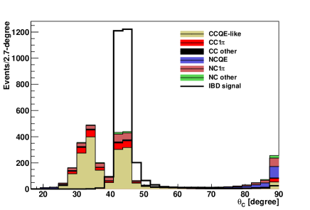
The opening angle of the Cherenkov light cone () emitted by highly relativistic particles, electrons and positrons in the current context, in pure water is around . Conversely, at the MeV energies considered here, heavier particles like muons and pions will be typically observed near the Cherenkov threshold, leading to cones with smaller angles in the current analysis range. In addition, NCQE interactions with multiple photon emission can produce multiple overlapping Cherenkov cones, that will be reconstructed as a single cone with a particularly large opening angle Abe et al. (2014b, 2019). Consequently, is one of the most powerful observables for reducing both NCQE and -producing atmospheric backgrounds. The Cherenkov angle distributions for the signal and atmospheric neutrino events are shown in Fig. 12 for the energy ranges of the model-independent analysis and the spectral analysis. In what follows we will require the Cherenkov angle in the signal regions to be in . In the spectral analysis, we will also use this angle to define sidebands to evaluate atmospheric backgrounds.

V.3.4 Ring clearness
Electrons and positrons do not follow a straight trajectory in SK due to scattering and bremsstrahlung, which leads to fuzzy Cherenkov rings. Pions, on the other hand, lead to well-delineated ring patterns. In order to characterize this property we consider a -ns time-of-flight subtracted window around the main activity peak and compute the opening angles of the cones formed by the directions of all possible 3-hit combinations. We then identify the peak of this opening angle distribution and estimate the “clearness” of the ring by computing:
| (4) |
The distributions from the atmospheric and IBD Monte-Carlo simulations are shown in Fig. 13. Events with lower have fuzzier rings. For the analyses presented here we require .


V.3.5 Average charge deposit
Energetic muons scatter less than electrons and hence often deposit more charge in individual PMTs than MeV electrons and positrons. We exploit this feature by considering a -ns time-of-flight subtracted window around the main activity peak and calculate the average charge deposited per PMT hit () in this window. The distributions are given in Fig. 14. We require to be less than in the analysis.


V.3.6 Cut efficiencies and systematic uncertainties
We estimate the signal efficiencies of most of the cuts detailed above using the IBD Monte-Carlo simulation. Hence, the main source of systematic uncertainties on the cut efficiencies stems from the modeling of the SK detector and particle propagation in water. We estimate these uncertainties using calibration data taken by injecting a monoenergetic electron beam produced by a LINAC at different positions inside the detector Nakahata et al. (1999). For a given cut, we compare the measured and predicted efficiencies using a dedicated Monte-Carlo simulation, and define the systematic uncertainty as the maximum discrepancy over all calibration tests. LINAC calibration thus allows to estimate uncertainties for ring clearness, the average charge, and Cherenkov angle cuts. Conversely, for the incoming event cut —that requires considering uniformly distributed events— we use a strategy developed for the SK solar neutrino analyses Hosaka et al. (2006); Cravens et al. (2008); Abe et al. (2011, 2016): we measure the variation of the cut efficiency after shifting the event directions and vertices in the IBD Monte-Carlo simulation. The vertex and direction shifts used for these estimates are obtained from calibration studies using a nickel source Abe et al. (2014a). Finally, efficiencies for the pre- and post-activity cuts can be directly estimated using a spallation-dominated sample of low energy events, with negligible systematic uncertainty. Overall, positron candidate selection cuts allow to remove a large fraction of atmospheric backgrounds while keeping up to 85% of the signal. The total systematic uncertainty computed for positron candidate selection cuts using these procedures are of a few percent.
V.4 Neutron tagging
The introduction of a new trigger scheme at SK-IV has made characterizing IBDs via neutron tagging possible, by requiring the prompt and delayed signals be detected within 500 s of each other. In what follows, we will devise a neutron tagging algorithm tailored to the DSNB analysis, inspired by previous SK studies from Refs. Zhang (2012, 2015).
V.4.1 DSNB candidate selection and neutron preselection
As explained in Section II, most SHE triggered events are followed by a 500 s AFT trigger window in order to record the neutron capture signal. Before attempting to identify neutron candidates in this combined trigger window, we apply a cut on the maximum hits inside a -ns window: to eliminate SHE+AFT trigger windows containing muons. This cut is associated with a signal efficiency larger than %. After applying the cut we scan the SHE+AFT trigger windows of the remaining events to select hit clusters that could be associated with neutron captures. Here, we take advantage of the fact that a typical neutron capture vertex is within a few tens of centimeters of the well-reconstructed IBD vertex. Since the SK resolution is about 50 cm for MeV events, this proximity allows to reliably estimate the required photon emission time for each PMT hit to be the result of the neutron capture. A neutron candidate is therefore defined as a group of hits that is clustered in emission time. We then look for clusters maximizing , the number of hits in a -ns window.
In previous SK-IV searches, neutron candidates were defined as clusters of hits satisfying Zhang (2012). This preselection cut has an efficiency of around and was motivated by the energy range of these searches, where spallation backgrounds were largely dominating. In this study, we modify this preselection step as follows. First, we apply a cut to reduce the continuous PMT dark noise, likely due to scintillation in the PMT glass, that causes a single PMT to flash more than once in rapid succession with a timescale of 10 s. To do so, for each PMT we remove hit pairs separated by less than 6 (12) s for (). After applying this cut, we define neutron candidates as hit clusters verifying . This preselection cut will allow loosening of the neutron tagging cut in energy regions where spallation no longer dominates, in particular for the spectral analysis. Finally, since the continuous dark noise cut relies on investigating PMT hit pairs, its efficiency sharply increases near the edge of the SHE+AFT trigger window. We restrict the neutron search window to [] s ([] s for events with a 350-s AFT trigger window). After these different steps, neutron candidate preselection is associated with an efficiency of .
V.4.2 Boosted Decision Tree
After preselection, we are still left with a large background from e. g. dark noise fluctuations and radon decays Nakano et al. (2020), totaling about 7 neutron candidates per event. To further reduce this background, for each neutron candidate, 22 discriminating variables are calculated. These variables are related to specific features of noise events (such as clustered PMT hits), the Cherenkov light pattern of the neutron candidate, and its position with respect to the primary event vertex. These observables are then used in a Boosted Decision Tree (BDT) implemented using the xgboost Python library Chen and Guestrin (2016). The BDT is trained using a data set of neutron candidates. In this sample, about candidates are neutron captures simulated using the procedure described in Section III.2 and the rest is composed of low energy accidental coincidences from random trigger events. Table 2 summarizes the BDT training parameters. The final BDT performance is shown in Fig. 15. Even accounting for preselection cuts, this neutron tagging algorithm allows reduction the background rate by a factor of compared to the analysis presented in Ref. Zhang (2015) for the same signal efficiency.
| Parameter | Value |
|---|---|
| learning rate | 0.02522 |
| subsample | 0.97 |
| max depth | 10 |
| tree method | approx |
| max iterations | 1500 |
| best iteration | 1170 |

V.4.3 Systematic uncertainty on neutron tagging efficiency
To estimate the systematic uncertainty on the BDT efficiency associated with mismodeling of neutron propagation in water and the MeV photon emission, we compare the efficiencies predicted by the IBD Monte-Carlo simulation to measurements performed using an americium-beryllium (241Am/Be) radioactive source embedded in a BGO scintillator. A detailed description of this procedure is given in Ref. Watanabe et al. (2009). To calculate the neutron identification efficiency for data, we follow the methodology described in Ref. Abe et al. (2021b) and fit the timing distribution of tagged neutrons by a decaying exponential plus a constant term as shown in Fig. 16. True neutron capture event counts decay exponentially in time from the detection time of the prompt event, while uncorrelated backgrounds are constant in time. By comparing the efficiency in data and simulation for BDT cut points relevant in our analysis, as described in Appendix B, we assign a relative uncertainty of for all neutron tagging cuts.

V.5 Solar neutrino cut
Since even mild neutron tagging cuts can reduce solar neutrino backgrounds to negligible levels, dedicated solar neutrino cuts are not implemented for the DSNB model-independent analysis. For the spectral analysis, however, events with no tagged neutrons are also considered in order to maximize the effective exposure. When considering these events, we hence apply additional cuts specifically targeting solar neutrino backgrounds. These cuts are based on the opening angle between the reconstructed direction of candidate events and the direction of the Sun. The cosine of this angle is peaked at 1 for solar neutrino interaction products, and is smeared by kinematic and reconstruction effects. To estimate the impact of the latter, an specific observable, the Multiple Scattering Goodness (MSG) has been designed for the solar neutrino analysis Hosaka et al. (2006); Cravens et al. (2008); Abe et al. (2011, 2016). Simulated opening angle distributions for solar neutrino events in different MSG bins are shown in Fig. 17.

In this analysis we use the method described in Ref. Bays et al. (2012) and apply cuts in the four MSG bins shown in Fig. 17. We estimate the impact of these cuts on DSNB signal events by assuming that these events have a uniformly distributed , and we obtain the associated MSG distributions using the IBD Monte-Carlo simulation. Conversely, to estimate the number of solar neutrino events above 15.5 MeV, we evaluate the number of solar events in 13.5-15.5 MeV from data and extrapolate the result to higher energies using the solar neutrino MC simulation from Ref. Abe et al. (2021c), a procedure already used in the DSNB search at SK-I,II,III Bays et al. (2012). Here, we can safely assume the distribution for non-solar event to be uniform Abe et al. (2016), and therefore approximate the number of solar events in 13.5-15.5 MeV by:
| (5) |
using the data passing the noise, spallation, and positron selection cuts described in Secs V.1, 3, and V.3. Using the solar neutrino MC simulation from Ref. Abe et al. (2021c), the predicted number of solar neutrino events above 15.5 MeV will then be:
| (6) |
The impact of solar and neutron tagging cuts can then be assessed by rescaling by the corresponding efficiencies.
Finally, we evaluate the systematic uncertainties on the signal efficiency with the solar event cut using the LINAC calibration results. Specifically, we compute the scaling factor that allows to minimize the difference between the predicted and observed MSG distributions for LINAC events. We then evaluate the impact of this rescaling on the final efficiency to be of about 1%.
V.6 Cut optimization
In this study, we perform two types of analyses. Here we adopt a common cut optimization procedure for both analyses.
V.6.1 DSNB positron candidate selection cuts
We determined the positron candidate selection cuts by comparing the IBD Monte-Carlo simulation with the atmospheric neutrino simulation for the ring clearness, average charge deposit, and Cherenkov angle, and the observed data for the effective distance . Since the impact of the positron candidate selection cuts depends weakly on the DSNB model considered, we assumed the Horiuchi09 spectrum Horiuchi et al. (2009). As discussed in Section V.3, we estimate systematic uncertainties using results from the solar neutrino analysis Hosaka et al. (2006); Cravens et al. (2008); Abe et al. (2011, 2016) and the LINAC calibration Nakahata et al. (1999). The final cuts are the following:
The efficiencies of these cuts are shown in Fig. 18 as a function of and vary between 70 and 85%. Overall, positron candidate selection cuts allow to remove of the atmospheric neutrino backgrounds, and bring contamination from natural radioactivity to negligible levels.
V.6.2 Spallation and neutron tagging cuts
Unlike positron candidate selection cuts, spallation and neutron tagging cuts need to be optimized in multiple energy regions to account for the important variations of the spallation and atmospheric background rates in the analysis windows. While only events with one tagged neutron are used in the DSNB model-independent analysis, the spectral analysis also considers events with zero or more than one tagged neutron. Here, we first optimize spallation and neutron tagging cuts for the signal region where exactly one tagged neutron is required. Using the thus optimized neutron tagging cuts, we then derive optimal spallation cuts for events with 1 tagged neutron.
Events with one tagged neutron:
We devise a cut optimization scheme common to both the model-independent and spectral analyses by simultaneously adjusting spallation and neutron tagging cuts in bins. For each energy bin, we select events with exactly one tagged neutron and find the spallation and neutron tagging cuts that yield optimal sensitivity under the background-only hypothesis. We define the sensitivity as the predicted number of signal events after cuts over the 90% C.L. upper limit on the number of signal events, computed using the Rolke method Rolke et al. (2005). To simplify the interpretation of the results presented in this paper, we apply the same cuts for both the model-independent and spectral analyses in the 15.529.5 MeV reconstructed energy range, where the two analyses overlap. In particular, we require spallation and solar neutrino backgrounds to be negligible above MeV. The remaining rates of these backgrounds can be reliably evaluated by rescaling the number of events observed after noise reduction, spallation, and positron candidate selection cuts by the neutron mistag rate.
The signal efficiencies for our choice of cuts are shown in the top panel of Fig. 18 for each energy region. For each set of cuts we also present the associated systematic uncertainties, computed as described in Sections V.2, V.3, and V.4, in Table 3.


| Cut | Relative systematic error |
|---|---|
| Spallation cut | |
| cut | |
| cut | |
| cut | |
| cut | |
| Neutron tagging | |
| Solar neutrino cut | % |
Events with zero or more than one tagged neutrons:
As previously discussed, the events rejected by the neutron tagging cuts obtained above can still be considered in the spectral analysis. In the 23.579.5 MeV region, that covers most of the spectral analysis window, spallation and solar neutrino backgrounds are negligible and only noise reduction and positron candidate selection cuts need to be applied to these events. In the 19.523.5 MeV region, solar neutrino backgrounds are still negligible and spallation backgrounds are mostly linked to short-lived isotopes, that are easy to reject using the cuts from Section V.2. For these energies, we therefore apply the spallation cut derived above, whose efficiency is close to 90%. In the 15.519.5 MeV range, however, both solar neutrino and spallation backgrounds largely dominate and need to be reduced using the targeted reduction strategies described in Sections V.2 and V.5. In this analysis, we remove the solar neutrino backgrounds using the cuts in Section V.5 with the cut points from Ref. Bays et al. (2012). The cut points and the corresponding signal efficiencies are shown in Table 4 for the different multiple scattering goodness and reconstructed kinetic electron energy regions. The remaining number of solar neutrino events after all cuts is less than 2 for the entire energy region.
| [MeV] | 15.516.5 | 16.517.5 | 17.518.5 | 18.519.5 |
|---|---|---|---|---|
| 0.05 | 0.35 | 0.45 | 0.93 | |
| 0.39 | 0.61 | 0.77 | 0.93 | |
| 0.59 | 0.73 | 0.81 | 0.93 | |
| 0.73 | 0.79 | 0.91 | 0.93 | |
| Efficiency | 73.1% | 82.2% | 88.3% | 96.6% |
In contrast, the impact of spallation cuts is difficult to evaluate in the 15.519.5 MeV range . To optimize spallation cuts for the events considered here, we therefore proceed as follows. First, we bring contributions from short-lived isotopes —with sec half-lives— to a negligible level, using the cuts shown. in Appendix A. As can be seen in Fig. 3, the remaining event sample will be dominated by decays from 8B and 8Li, that have a half-life close to 1 sec. We then optimize the spallation likelihood cuts using the method described in Appendix A.4 to compute the remaining amount of 8B and 8Li decays, and maximize where and are the numbers of spallation and non-spallation events respectively. The efficiencies of the optimal cuts are of 65% and 63% in 15.517.5 and 17.519.5 MeV, for a 8B+8Li remaining fraction of about 2.5%. The corresponding remaining number of spallation events, as well as the performance of this cut will be discussed and compared to results from the previous SK DSNB analyses in Section VII.5.
V.7 Selected events in the final data samples
Here we discuss the behavior of the observed data after the cuts. In particular, the impact of spallation, , and the other positron candidate selection cuts on data is shown in Fig. 19. As shown in this figure, for reconstructed energies below 20 MeV contributions from spallation and radioactivity near the wall are significant. To validate our background modeling and neutron tagging procedure we also compare the observed data to the background expectations after the noise reduction, multiple spallation cuts, DSNB positron candidate selection, and neutron tagging cuts. To simplify the interpretation of the data, we impose the same neutron tagging cut, with a 20% signal efficiency, for all energies. While most spallation cuts are removed in order to focus on neutron tagging, multiple spallation cuts are conserved in order to avoid contaminating the neutron detection window with isotope decays —an effect not accounted in the mistag rate predictions. The predicted and observed event spectra are shown in Fig. 20 and agree within uncertainties.
After the cuts derived in Section V.6 are applied, we find 102 events with exactly one neutron in 7.579.5 MeV. For these events, the distribution of the time difference between the neutron and the prompt event is shown in Fig. 21. Fitting this distribution by an exponential plus a constant, as is done in the 241Am/Be calibration, yields a time constant of s, which is compatible with the expected neutron capture time in water. In the 15.579.5 MeV region, that will be used for the spectral analysis, we also find 248 events with zero neutrons and 9 events with more than one neutron. The observation times and reconstructed vertices for these events are shown in Figs. 22 and 23. No event time cluster has been observed and the time-dependence of the event rate is consistent with the livetime variations over the SK-IV period. Events are also uniformly distributed all over the FV, irrespective of the number of neutrons. The space and time distributions of the selected events are therefore consistent with what is expected for DSNB candidates.


VI DSNB Model-independent Analysis
In this section we perform a DSNB model-independent search. Specifically, we divide the 7.529.5 MeV reconstructed energy range into -MeV bins and, in each of them, search for DSNB IBDs. In what follows, we describe how to estimate the various backgrounds encountered in this analysis, model their energy dependence, and estimate the corresponding uncertainties.
VI.1 Background estimation
VI.1.1 Atmospheric neutrinos
In the high end of the analysis window ( MeV), the atmospheric neutrino spectrum is dominated by decay of invisible muons or pions from CC or NC interactions, forming the well-known Michel spectrum. Systematic uncertainties in this region will therefore only affect the total number of predicted atmospheric neutrino events. Here, we estimate this number using the sideband region of MeV, that has a similar background composition. The number of events in this sideband is of the atmospheric neutrino Monte-Carlo prediction, and we therefore use this factor to rescale the non-NCQE backgrounds. The associated uncertainty is due to statistical fluctuations in the number of events in the sideband and is around %. The resulting spectrum is labeled as “non-NCQE” in Fig. 24.
Below MeV, the dominant atmospheric neutrino background arises from NCQE interactions. The cross section measurements from T2K Abe et al. (2019) are used to estimate this background. In particular, the Monte-Carlo simulation predictions of neutrino and antineutrino NCQE interactions are renormalized using the scaling factors from this measurement; and , respectively. Note that this rescaling provides an inclusive estimation of the NCQE and NC 2p2h interactions. The errors of these factors are taken as cross section uncertainties.
Two additional flux uncertainties are considered for the NCQE background: the atmospheric neutrino flux uncertainty and the uncertainty due to the flux difference between the T2K beam and atmospheric neutrinos. For the former, a % uncertainty is taken from Refs. Honda et al. (2007, 2011). The latter uncertainty arises from the fact that the scaling factors above are measured for the T2K fluxes while the current focus is the atmospheric neutrino flux and then the effect of cross section model uncertainties is different. To estimate this uncertainty, the ratios of flux-averaged events in the T2K beam and atmospheric neutrino fluxes for different cross section models are calculated. Here six models are considered: Spectral Function (SF) Benhar et al. (1994, 2005), Relativistic Mean Field (RMF) Horowitz and Serot (1981); Maieron et al. (2003); Caballero et al. (2005); Gonzalez-Jimenez et al. (2013), Superscaling (SuSA) Amaro et al. (2005, 2006), Relativistic Green’s Function (RGF) Capuzzi et al. (1991); Gonzalez-Jimenez et al. (2013); Meucci et al. (2004); Meucci and Giusti (2014) with two functional forms for the potential (EDAI, Democratic), and Relativistic Plane Wave Impulse Approximation (RPWIA) Gonzalez-Jimenez et al. (2013). The maximum differences are taken as systematic errors, 5% for neutrinos and 7% for antineutrinos.
There are two systematic error sources related to neutron tagging for the NCQE background: tagging efficiency and neutron multiplicity. For the uncertainty on the tagging efficiency, 12.5% is employed in this analysis as the maximum difference between the measured and predicted efficiencies in the 241Am/Be calibration. The neutron tagging efficiency will also depend on the distance between the neutron emission and capture vertices. Indeed, neutrons produced in atmospheric interactions can travel up to a few meters and are hence more difficult to identify than neutrons produced in DSNB IBDs. The effect of the uncertainties in modeling the neutron travel distance on the efficiency is of around % Wan et al. (2019). In this analysis, the number of tagged neutrons is required to be one, therefore the model uncertainty affecting the neutron multiplicity has to be estimated. Here the recent measurement of the neutron multiplicity after (mostly CC) interactions of neutrinos from the T2K beam inside the SK tank is used Akutsu (2019). This measurement allows to compare observations with Monte-Carlo simulation predictions for neutron multiplicity as a function of the reconstructed squared momentum transferred to the nucleus, , and could therefore be adjusted to study the NCQE background. We incorporate the maximum difference between observed and predicted neutron multiplicity in T2K for each range, and renormalize the present Monte-Carlo simulation prediction to accommodate this gap. This procedure gives variances of approximately 40% in the number of events with the tagged neutron being one, both for neutrinos and antineutrinos.
The NCQE spectral shape is sensitive to the emission model, affecting the current differential limit extraction. It is complicated to estimate the associated systematic uncertainty, as rays are produced at every stage of the NCQE process, from the primary neutrino interaction to the secondary nuclear reaction. The modeling of these emission is in particular a probable cause of the currently observed discrepancy between the observed and predicted Cherenkov angle distributions using neutrinos from the T2K beam Abe et al. (2019). One notable effect of this mismodeling is a smearing of the reconstructed energy analogous to a resolution effect. To evaluate the associated systematic uncertainty we model this smearing by convolving the original spectrum with a Gaussian distribution and using the energy-dependent ratio between the smeared and unsmeared spectra to renormalize the Monte-Carlo events. We then compute the number of renormalized events in each energy bin after the reduction steps described in Section V. The difference between this result and the nominal prediction is then taken as the systematic uncertainty associated to the emission modeling. For this study, we set the smearing parameter to 3 MeV for all energies; this value allows to cover the discrepancy observed between the predicted and observed distributions in the T2K measurements mentioned above. The resulting uncertainty ranges from 30% to 60% in the 7.529.5 MeV range.
Finally, we combine all the systematic uncertainties described above by adding them in quadrature. The total systematic uncertainty on the NCQE background then varies from 60% to 80% for low to high energies. The predicted NCQE spectrum with the T2K scaling is shown in Fig. 24.
VI.1.2 Spallation 9Li
The background rate of spallation 9Li can be estimated by the following formula:
| (7) |
where is the production 9Li rate measured at SK () Zhang et al. (2016), is the operational livetime (2075.3 and 2970.1 days below and above MeV, respectively), is the branching ratio for + decay, is the fraction of the 9Li decay energy spectrum above the search energy threshold, and is the reduction efficiency. We estimate using the Monte-Carlo simulation elaborated for IBD events, renormalized to fit the 9Li spectrum. This same simulation can be used to estimate the efficiencies for the noise and positron reductions as well as the neutron tagging, that are the same as for the DSNB signal. The spallation cut efficiency is estimated using the procedure outlined in Section V. The dominant systematic uncertainty on the number of 9Li events in each energy bin after cuts arises from estimating the impact of spallation cuts. Indeed, as discussed in Appendix A.4, our method assumes that the time difference between an isotope decay and its parent muon is the only isotope-dependent spallation observable. In this study, we account for the impact of other spallation observables by defining a 50% uncertainty on the number of 9Li events. The uncertainty on the event rate is taken from the previous SK study Zhang et al. (2016) as 22%. Other uncertainties come from the reduction, especially from the spallation cut and neutron tagging, that is 20% in total. The total uncertainty assigned for the 9Li background estimation is therefore 60%.
VI.1.3 Reactor neutrinos
Reactor neutrino backgrounds are estimated by renormalizing the IBD Monte-Carlo simulation. They populates only in the lowest energy bin, as seen in Fig. 24. In this analysis, a conservative 100% uncertainty is assigned to their estimated rate.
VI.1.4 Accidental coincidences
A prompt SHE signal accidentally paired with a subsequent dark noise fluctuation or a low energy radioactive decay can look like an IBD signature. Since accidental pairing can occur for both signal and background events, the resulting background can be readily estimated by computing the number of events left after noise reduction, spallation, and positron reduction cuts , and rescaling it by the neutron mistag rate:
| (8) |
The associated systematic errors are highly cut-dependent and arise from the time dependence of the PMT dark noise and natural radioactivity. In order to evaluate its effect on the background rejection, we separate the random trigger data mentioned in section III.2 over all the SK-IV period into time bins of about eight months each. Then we evaluate the BDT mistag rate for each bin separately and, for a given signal efficiency, take the standard deviation from the average mistag rate as systematic error. The typical size of uncertainty is a few to %, in the region of interest for the DSNB analyses, as shown in Fig. 15.
VI.2 Differential upper limit
The observed data and expected background spectra are shown in Fig. 24. The corresponding p-values are calculated for each energy bin by performing pseudo experiments as follows. We vary the number of expected background events randomly based on Gaussian distributions with their widths being the 1 systematic uncertainties from each background source. We then calculate p-values from the resulting distributions and the observed number of events in each bin, as shown in Table 5. Here the most significant bins are found to be at 2 level. We therefore conclude that no significant excess is observed in the data over the background prediction in any energy bin, and place upper limits on the extraterrestrial flux using the pseudo experiments above. Here we obtain the 90% C.L. upper bound on the number of signal () as an excess of the observation over the background expectation, by varying the number of observed events in each energy bin by their statistical uncertainties as well as varying the number of expected background events by their systematic uncertainties from each source. The 90% C.L. upper limit on the flux is then calculated as:
| (9) |
where is the operational livetime [sec], is the number of free protons in the SK’s FV, is the IBD cross section [] at a mean neutrino energy in the corresponding region (), and is the signal efficiency. Note that the neutrino energy is obtained as MeV in IBD. For the expected sensitivity, the same procedure is applied while the number of observed event is replaced with the number of nominal background prediction. Here statistical uncertainties on the backgrounds are considered instead. The expected sensitivities and observed upper limits from this work are summarized in Table 5. These results are also compared with the previously published results and theoretical predictions in Fig. 25. Note that the SK-I,II,III limits presented in this figure have been obtained using a different methodology, more similar to the one used for the spectral analysis in Section VII. In addition, the SK-I,II,III analysis not only used a higher energy threshold but also did not involve neutron tagging Zhang (2012); Bays et al. (2012). Hence, we do not combine the SK-IV result with the SK-I,II,III one for the model-independent differential limit. The sensitivities obtained with this analysis are the world’s tightest above neutrino energies of 11.3 MeV. The current limit disfavors the Totani95 model Totani and Sato (1995) and the most optimistic predictions of the Kaplinghat00 model Kaplinghat et al. (2000), and is reaching close to several other model predictions. Due to not only a higher exposure but also higher cut efficiencies and more precise background estimation, this new analysis considerably improves on the previous SK-IV DSNB model-independent search Zhang (2012).


| [MeV] | Expected [] | Observed [] | p-value |
|---|---|---|---|
| 9.311.3 | |||
| 11.313.3 | |||
| 13.315.3 | |||
| 15.317.3 | |||
| 17.319.3 | |||
| 19.321.3 | |||
| 21.323.3 | |||
| 23.325.3 | |||
| 25.327.3 | |||
| 27.329.3 | |||
| 29.331.3 |

VII Spectral fitting
In this section, we derive model-dependent limits on the DSNB flux by fitting signal and background spectral shapes to the observed data in the 15.579.5 MeV range, and combine the results with the ones from previous SK phases Bays et al. (2012) to achieve a ktonday exposure. While atmospheric neutrino backgrounds, notably from decays of invisible muons and pions, will dominate over most of the analysis window, we also account for possible residual spallation in 15.519.5 MeV.
VII.1 Signal and sideband regions
In order to evaluate the number of atmospheric neutrino background events, we define three regions of parameter space based on the reconstructed Cherenkov angle: one signal region with , that will contain most of the signal and the irreducible backgrounds, and two sidebands with and . The low Cherenkov angle region will be populated with mostly atmospheric backgrounds involving visible muons and pions while the high angle region will be mostly populated by NCQE atmospheric neutrino events with multiple rays. Finally, we separate events with exactly one identified neutron from the others, thus defining an “IBD-like” and a “non IBD-like” region. Note that due to the low efficiencies of the neutron tagging cuts the non IBD-like region is expected to contain a sizable amount of signal. Our analysis will hence involve six regions of parameter space: two signal regions with intermediate values of the Cherenkov angle, and four sidebands with low and high Cherenkov angle values, as summarized in Table 6.
| 2038∘ | 3850∘ | 7890∘ | |
| 1 | I | II | III |
| 1 | IV | V | VI |
VII.2 Spectral shape fitting
We perform a simultaneous fitting of the signal and background spectra to the observed data in all six regions of parameter space defined in Table 6 using an extended maximum likelihood method. Performing this type of analysis requires knowing the shapes of the signal and background spectra in each of the regions. While the signal spectrum can be reliably predicted by the IBD Monte-Carlo simulation for a given DSNB model, the treatment of the atmospheric neutrino and spallation backgrounds is more complex. For this study, we follow the method described in Ref. Bays et al. (2012) and divide these backgrounds into the following five categories.
Invisible muons and pions:
this category regroups events with electrons produced by the decays of invisible muons and pions. The energy distribution of these electrons follows a Michel spectrum, whose shape is independent of the Cherenkov angle and the neutron multiplicity and will therefore be the same across all six regions. For this study, we estimate the shape of the Michel spectrum at SK directly from data, using a sample of electrons produced by cosmic ray muon decays (a similar sample for atmospheric and accelerator neutrino oscillation and proton decay analyses is described in Refs. Ashie et al. (2005); Regis et al. (2012)). We then use the atmospheric neutrino Monte-Carlo simulation to compute the fractions of background events in the different signal and background regions. Since electrons cannot be distinguished from positrons at SK this background dominates in the signal regions II and V and are negligible everywhere else.
CC interactions:
in this category we find backgrounds arising from CC interactions of electron neutrinos and antineutrinos, with no visible muons and pions in the final state. Their contributions will dominate in the signal regions II and V above MeV. We estimate the associated spectral shapes in all regions using the atmospheric neutrino Monte-Carlo simulation. Similarly to Michel electrons, this background is negligible outside the regions II and V.
-producing interactions:
visible muons and pions will be associated with low Cherenkov angles, as these particles are significantly heavier than electrons. The associated background will therefore dominate in the low Cherenkov angle regions I and IV, and, after positron candidate selection cuts, will be negligible in the signal regions. We extract the associated spectral shapes by considering an atmospheric Monte-Carlo sample with only CC interactions, visible muons and pions, and no electrons.
NCQE interactions:
unlike the other types of atmospheric neutrino events the NCQE spectrum peaks at low energies, similarly to the DSNB spectrum. Here we define spectral shapes using simulated NCQE events with no electrons. This background, often involving multiple rays, will dominate in the high Cherenkov angle regions III and VI, but will also contribute to all other regions.
Spallation backgrounds:
these backgrounds are negligible in the one-tagged-neutron regions I, II, and III after the cuts. However, in the other regions, especially in signal region V, residual spallation backgrounds from 8Li, 8B, and 9C decays could remain. Since 9C has a shorter half-life and is produced closer to the muon track than the other two isotopes, it is expected to be subdominant. To model the spallation spectrum and its variability we parameterize this spectrum and vary its isotope composition as follows:
| (10) | ||||
where refers to the decay spectrum for a given isotope , normalized to one in the spectral analysis energy window, and and are the isotope fractions. Here, we constrain 9C to always be less abundant than the other two isotopes after spallation cuts are applied. In what follows, we will take the nominal spallation spectrum to be the average between the steepest and the least steep spectra and parameterize possible deviations from this hypothesis as systematic uncertainties. We evaluate the spectra using external measurements Winter et al. (2006) for 8B decays and GEANT4 for 8Li and 9C. As with 9Li, we then use these spectra to renormalize events in the IBD Monte-Carlo simulation and thus model detector resolution effects.
Although the first four background categories do not include all possible types of atmospheric neutrino interactions, their associated spectra can be linearly combined to model other background categories. Pion-producing NC backgrounds can notably be treated as a superposition of NCQE and decay electron backgrounds. The five categories described here hence allow to map all the background configurations relevant to this analysis.
For each background category we define probability distribution functions (PDFs) which model the corresponding energy spectra in each of the six Cherenkov angle and neutron regions. These PDFs are normalized to across all regions. We apply a similar procedure to obtain signal spectral PDFs associated to different DSNB models, using the IBD Monte-Carlo simulation. For observed events with energies we then extract the most probable numbers of signal and background events by performing an extended unbinned maximum likelihood fit, using the following likelihood function:
| (11) |
Here, the index refers to the signal and the five background categories described above. Then designates the numbers of events for the signal and the different background types, across all six Cherenkov angle and tagged neutron regions. For each event, is the PDF for the signal or background category in the region (for the regions defined in Table 6).
VII.3 Systematic uncertainties
One considerable advantage of using the likelihood defined in Equation 11 is that the sizes of the different background contributions can be treated as nuisance parameters. This likelihood, however, does not account for the considerable uncertainties on the spallation and atmospheric background spectral shapes in the energy window of the DSNB analysis. In this section, we outline how to incorporate systematic uncertainties on these shapes as well as on detector modeling and predicted cut efficiencies. We account for systematic uncertainties on the spallation and atmospheric neutrino background spectral shapes, energy reconstruction, and reduction efficiencies by convolving the likelihood introduced in Equation 11 with suitable probability distributions. Here we neglect the systematic uncertainties associated with the background. The amounts of these background in the signal regions II and V are indeed constrained to be negligible by observations from the low angle regions I and IV, a result that is robust under large variations of the assumed spectral shapes in these regions. We also neglect the systematic uncertainties on the spectral shape of the background associated with invisible muon and pion decays since this shape has been directly extracted from a large sample of SK-IV data. We then consider five sources of systematic uncertainties: energy scale and resolution, spectral shape predictions for the spallation, NCQE, and CC backgrounds, and reduction cut efficiencies.
VII.3.1 Energy scale and energy resolution
To estimate the impact of energy scale and energy resolution uncertainties on the signal and atmospheric background spectra, we follow the procedure described in Ref. Bays et al. (2012). The energy scale and energy resolution uncertainties are obtained from the solar neutrino analysis and increased to 2% and 3% respectively to account for the higher energies studied here. We model the effect of these uncertainties by distorting the signal and atmospheric background PDFs in Equation 11 using the energy resolution functions from Refs. Hosaka et al. (2006); Cravens et al. (2008); Abe et al. (2011, 2016). We parameterize the amount of distorsion applied to these PDFs using the variable such that represents a deviation in the energy scale and resolution. The final likelihood can then be expressed as:
| (12) |
where represents the likelihood from Equation 11 with the PDFs distorted by an amount . These uncertainties have a negligible impact on the final result and are therefore not taken into account in the final fit.
While energy scale and resolution uncertainties on signal and atmospheric background spectra can be neglected in this analysis, the spallation background spectrum is particularly steep and hence more sensitive to the modeling of energy reconstruction. In this analysis, we will therefore account for the associated modeling uncertainties when estimating spallation spectral shape systematic uncertainty.
VII.3.2 Spallation background spectral shapes
As discussed above, we consider two sources of systematic uncertainties here: energy scale and resolution uncertainties, and isotope composition. We estimate the latter by varying the 8B, 8Li, and 9C fractions as shown in Equation 3. Then, we distort the steepest and least steep spectra found using this method in order to account for the 2% and 3% energy scale and resolution uncertainties discussed above. We take these distorted spectra as our 1 variations from the nominal spallation spectrum. Finally, we parameterize the total spectral distorsion associated with the systematic uncertainty by using a third order polynomial such that:
| (13) |
where is expressed in units of . More details about these estimates are given in Appendix D. We then convolve the likelihood from Equation 11 with a Gaussian prior on :
| (14) |
VII.3.3 Atmospheric CC spectral shapes
The shape of the CC background for electron energies below about MeV has not been studied in-depth to date, although Monte-Carlo simulations predict a linear increase in the number of events with the electron energy. In our analysis, we model this spectral shape uncertainty by allowing the slope of the CC spectrum to vary in the two signal regions. We then integrate the distorted PDF using pseudo-Gaussian weights. A detailed description of this procedure is provided in Ref. Bays et al. (2012).
At this step of the analysis, we assume the spectral shape distortions in the 1 and 1 tagged neutron regions to be fully correlated and model the effect of neutron multiplicity uncertainties separately.
VII.3.4 Relative normalization for NCQE events
The Cherenkov angle distribution of atmospheric NCQE events is associated with large uncertainties stemming from the modeling of ray emission. We incorporate this uncertainty in the current analysis by allowing the relative normalization of the NCQE PDFs between the different Cherenkov angle regions to vary. Following the procedure outlined in Ref. Bays et al. (2012), we define a 1 variation of this normalization to correspond to a change of the number of NCQE events in the intermediate Cherenkov angle region. Additionally, in order for the overall normalization of the NCQE PDFs across regions to remain constant, we reweight these PDFs as follows:
| (15) | ||||
| (16) | ||||
| (17) |
where the “low”, “med”, and “high” indices refer to the low (2038∘), medium (3850∘), and high (7890∘) Cherenkov angle ranges from Table 6 and for the tagged neutron regions respectively. are scaling factors introduced to preserve the overall normalization of the PDFs. The parameterizes the PDF distortion, in units of . We finally inject these distorted PDFs into Equation 11 and convolve the new likelihood with a weighted Gaussian prior, as with CC background uncertainties.
VII.3.5 Uncertainty on the neutron multiplicity
The fractions of signal and background events observed in the 1 and 1 tagged neutron regions depend on both the neutron tagging efficiency and the true neutron multiplicity of the observed events. As shown in the 241Am/Be calibration study, the efficiency of the neutron tagging cut for the DSNB spectral analysis is associated with a systematic uncertainty of around %. Conversely, the actual neutron multiplicity for atmospheric neutrino interactions is poorly known. As discussed in Section VI.1, neutron multiplicity uncertainties of up to 40% have been measured for reconstructed energies above MeV using the T2K neutrino beam Akutsu (2019). In what follows, we therefore consider a systematic uncertainty on the neutron tagging.
We model the effect of neutron multiplicity uncertainties by varying the relative normalization of the PDFs in the 1 and 1 tagged neutron regions for the CC, NCQE, and invisible muon and pion backgrounds. As mentioned at the beginning of this section we neglect the systematic uncertainty associated with backgrounds, which are associated with negligible contributions in the signal region. As discussed above, we set the 1 variation of the fraction of events with one tagged neutron to a conservative value of . We then distort the PDFs in the 1 and 1 tagged neutron regions for each background category as follows:
| (18) | ||||
| (19) |
where is the relative systematic uncertainty for background category , measures the magnitude of the distortion in units of and preserves the overall normalization of the PDFs. Finally, we incorporate this uncertainty into the final likelihood by integrating the initial likelihood similarly to Equation 14.
VII.3.6 Combining the background uncertainties
The three categories of systematic uncertainties on backgrounds described above —spallation and CC spectral shapes, NCQE Cherenkov angle distribution, and neutron multiplicity— are incorporated into Equation 11 using the modified likelihood defined in Equation 14 and the modified PDFs defined in Ref. Bays et al. (2012) as well as in Eqs 17 and 19 with distorsion parameters , , and respectively. The final likelihood can then be written as:
| (20) | ||||
VII.3.7 Energy-independent efficiency systematic error
Maximizing the likelihood defined in Equation 20 over the numbers of events in all five background categories results in a marginalized likelihood where is the number of signal events. Using this likelihood to constrain the total number of DSNB events that passed through the detector, , requires rescaling by the average value of the signal efficiency over all analysis regions and their associated energy windows, . We therefore need to incorporate the systematic uncertainty on into , following a procedure similar to the treatment of the background systematic uncertainty. Since the neutron tagging efficiency only affects the relative normalization between regions, the main sources of uncertainties on will arise from noise reduction and positron candidate selection cuts. These uncertainties are summarized in Table 3. We also incorporate the uncertainties associated to the fiducial volume cut, inverse beta decay cross section, and livetime calculation, that have been taken from the solar neutrino analyses and are summarized in Table 7. Adding all these uncertainties in quadrature, we then rewrite the likelihood as:
| (21) |
where is the systematic uncertainty on .
| SK phase | I | II | III | IV |
|---|---|---|---|---|
| Fiducial volume | 1.3% | 1.1% | 1.0% | 1.5% |
| Cross section | 1.0% | 1.0% | 1.0% | 1.0% |
| Livetime | 0.1% | 0.1% | 0.1% | 0.1% |
Systematic uncertainties associated with reduction efficiencies weaken the final limits by around . Similarly, while the uncertainties associated with spallation and atmospheric neutrino backgrounds are of order , their overall effect on the final limits is of about . The limited impact of spectral shape uncertainties is due to the large dominance of backgrounds associated with invisible muon and pion decays, whose spectrum is well-known. The final analysis will hence be largely dominated by statistical uncertainties, which will allow to easily combine SK-IV observations with results from previous SK phases.
VII.4 Combination with SK-I,II,III
The methodology described above, based on an extended maximum likelihood fit over signal and sideband regions, is similar to the one described in Ref. Bays et al. (2012), that performed a DSNB spectral analysis over the ktondays of data corresponding to the first three SK phases. While this previous analysis did not include neutron tagging and used slightly different background categories and reduction cuts, it is also dominated by statistical uncertainties. Hence, the SK-I,II,III results can be readily combined with the SK-IV observations.
In order to study a wide variety of the discrete and parameterized models introduced in Section I, we build signal PDFs for all four phases of SK using Monte-Carlo simulation to model detector resolution effects over most of the energy range. For SK-IV, we renormalize the IBD Monte-Carlo simulation by the predicted DSNB spectrum for all energies. For SK-I,II,III, we renormalize the simulations used in Ref. Bays et al. (2012) —with events generated in in 1090 MeV— and use the resolution functions from Refs. Hosaka et al. (2006); Cravens et al. (2008); Abe et al. (2011) to extrapolate them to lower energies. For the Galais+10 Galais et al. (2010) and the Nakazato+15 Nakazato et al. (2015) models, for which DSNB fluxes are available only up to antineutrino energies of 50 MeV, we assume the predicted flux to be zero in the 5081.3 MeV range. This assumption is not expected to affect the spectral fit, as backgrounds from CC interactions largely dominate at these energies. Finally, for each DSNB model, we fit the data samples obtained in Ref. Bays et al. (2012) for the first three SK phases. Here, although we use the same cuts and search regions as in Ref. Bays et al. (2012), we account for possible residual spallation by modeling the spectra and associated systematic uncertainty using the same procedure as at SK-IV. We then combine the four fit results by summing the corresponding likelihoods maximized over the nuisance parameters.
VII.5 Results
We apply the procedure described in the previous sections to the observed data collected during phases I to IV of SK for the Horiuchi+09 DSNB model Horiuchi et al. (2009). The associated spectral fits for SK-IV and for SK-I,II,III are shown in Figs. 26 and 27 for the DSNB signal and for the spallation and atmospheric neutrino background categories introduced in Section VII.2. Since neutron tagging was not possible in the first three phases of SK, the corresponding fits span only three regions, defined by the low, medium, and high Cherenkov angle ranges defined in Table 6. For SK-IV, the low energy bump in the predicted decay electron spectrum for IBD-like events is due to the energy dependence of the neutron tagging cut, that strongly depends on the background composition. As expected, the dominant backgrounds in the low and high Cherenkov angle sidebands are backgrounds with visible muons and pions and NCQE backgrounds, respectively. While most of the signal region is dominated by backgrounds from invisible muons and pions, CC contributions become sizable above about 50 MeV. For SK-IV, the background rates are extremely low in the IBD-like region, that will hence be particularly sensitive to IBD signals in spite of the low efficiency of the neutron tagging cut.
In spite of introducing spallation backgrounds in the spectral fits, the results shown in Fig. 27 for SK-I,II,III are highly similar to the ones shown in Ref. Bays et al. (2012). The number of spallation events for each phase never exceed 2, within the upper limit obtained in Ref. Bays et al. (2012). Since the current analysis uses a similar procedure with more inclusive muon selection criteria and 2025% lower signal efficiencies, the spallation cut effectiveness at SK-IV should remain on par with the ones observed at previous SK phases. Yet, an important amount of spallation backgrounds (8 events) is predicted below 19.5 MeV at SK-IV. The origin of this important spallation background will be further studied in future SK analyses with an enhanced performance by gadolinium. Note that this effect was not observed in other SK searches probing a similar energy range. These searches however used specific cuts on e.g. the event timings or opening angles that we do not apply in this analysis.
Even accounting for possible residual spallation, the number of events observed in 17.519.5 MeV is higher than the best-fit predictions from Fig. 26. While this can be explained by statistical fluctuation, it led us to investigating possible non-spallation sources for the excess observed over atmospheric neutrino background predictions in 15.519.5 MeV. We first ruled out the possibility of a strong DSNB signal, as it would be associated with a steeply falling spectrum and hence to an unrealistically high supernova rate. The hypothesis of an isolated astrophysical event is also strongly disfavored since the observed events are uniformly distributed over the SK-IV period, as discussed in Section V.7. A radioactive origin for the observed events is also highly unlikely, given their high energies and their uniform spatial distribution. The event positions are notably not correlated with the locations of calibration sources. Residual spallation therefore remains the most plausible explanation for the high number of events observed in 15.519.5 MeV at SK-IV.
The likelihoods associated to the SK-I to IV fits for the Horiuchi+09 model are shown in Fig. 28 as a function of the DSNB rate for the reconstructed equivalent electron kinetic energies MeV. This figure also shows the likelihood for the combined analysis, with a total exposure of ktondays. The associated limits on the DSNB flux are shown in Table 8. The expected sensitivities of the SK-I,II,III analysis change by only 3% with the inclusion of the spallation backgrounds while the associated observed upper limits on the DSNB flux become tighter. The expected sensitivities of the SK-IV and the combined analyses to the DSNB flux at C.L. are cm-2 and cm-2, respectively. Hence, the predicted flux for this model, cm-2, is well within the reach of the SK-I,II,III,IV analysis. The observed upper limits on the DSNB flux for SK-IV and for the combined analysis are of cm-2 and cm-2, respectively. The best-fit flux for the combined analysis is now of cm-2. The 1.5 excess observed over the background prediction is higher than the 0.9 excess from the previous combined analysis Bays et al. (2012). While not statistically significant, this result is compatible with a wide range of DSNB predictions with a flux comparable to the one of the Horiuchi+09 model Horiuchi et al. (2009).


VIII Discussion
VIII.1 Constraints on the DSNB parameter space
Over the two search strategies presented in this paper, the analysis described in Section VI gives a model-independent differential limit on the flux while the model-dependent spectral analysis uses data from all phases of SK and yields the tightest constraints on DSNB models. In this section, we present the results of this analysis using both discrete DSNB models —most of them based on supernova simulations— and simplified parameterizations.
The C.L. expected and observed upper limits on the DSNB rate and flux for theoretical models are shown in Fig. 29 for the combined SK-I,II,III,IV analysis, with the corresponding results being tabulated in Table 8. With an exposure of ktondays, the sensitivity of the combined analysis at C.L. is the tightest to date and is on par with predictions from the Ando03, Horiuchi09 ( MeV), Galais10, and Kresse21 models Ando et al. (2003); Horiuchi et al. (2009); Galais et al. (2010); Kresse et al. (2021). One common feature of these optimistic models is that they use the highest cosmic star formation history allowed by observations. Additionally, the Kresse+21 predictions Kresse et al. (2021) are based on neutrino emission models derived from state-of-the-art supernova simulations, and take a wide range of progenitors into account. The ability of this analysis to probe such realistic models makes the prospects for future experiments particularly promising. Currently, an excess of about has been observed in the data and the resulting C.L. limits on the DSNB flux improve on the constraints obtained in Ref. Bays et al. (2012) for SK-I,II,III. These results confirm the exclusion of the Totani95 model Totani and Sato (1995) and of the most optimistic predictions of the Kaplinghat model Kaplinghat et al. (2000).

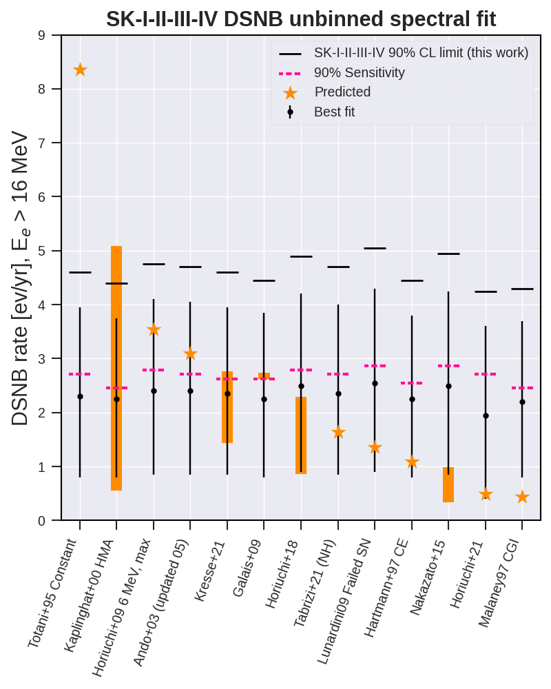
Another striking feature observed in Fig. 29 is the stability of the observed and expected limits on the DSNB flux over all models. This stability results from the limited sensitivity of the current analysis to the DSNB spectral shape. In order to translate flux limits into constraints on astrophysical parameters, we therefore ignore subtle effects associated with e.g. black-hole formation or multiple classes of progenitors, and use the simple Fermi-Dirac neutrino emission model described in Section III, as in Ref. Bays et al. (2012). The associated two-dimensional C.L. limit on the neutrino emission temperature and on the DSNB rate for MeV is shown in Fig. 30, for the combined SK-I,II,III,IV analysis. This figure also shows the expected rates for different effective neutrino emission temperatures. Here, the band accounts for the current uncertainty on the cosmic star formation rate, using the low, fiducial, and high estimates from Ref. Horiuchi et al. (2009). Since we used two-dimensional exclusion contours instead of computing limits for individual models, the limits appear weaker than the ones shown in Fig. 29. These limits are on par with the SK-I,II,III analysis Bays et al. (2012). In addition to the rate limits, whose interpretation is complicated by the high SK analysis threshold, we also show C.L. exclusion contours for the total energy and the effective neutrino temperature in Fig. 31. This figure also shows the regions of parameter space allowed by the Kamiokande II and IMB experiments for the supernova SN1987A Jegerlehner et al. (1996). While the neutrino temperature for this supernova is particularly low, future experiments should be able to probe at least the associated IMB region.


| Best fit | 90% CL limit | Pred. | ||||||
|---|---|---|---|---|---|---|---|---|
| Model | SK4 | All | SK1 | SK2 | SK3 | SK4 | All | |
| Totani+95 Constant | 2.5 | 1.3 | 2.3 | 6.3 | 7.0 | 4.5 | 2.6 | 4.67 |
| Kaplinghat+00 HMA (max) | 2.6 | 1.3 | 2.3 | 6.7 | 7.1 | 4.7 | 2.6 | 3.00 |
| Horiuchi+09 6 MeV, max | 2.6 | 1.3 | 2.4 | 6.0 | 7.0 | 4.6 | 2.6 | 1.94 |
| Ando+03 (updated 05) | 2.7 | 1.4 | 2.3 | 6.6 | 7.2 | 4.7 | 2.7 | 1.74 |
| Kresse+21 (High, NO) | 2.7 | 1.4 | 2.3 | 6.7 | 7.2 | 4.7 | 2.7 | 1.57 |
| Galais+09 (NO) | 2.5 | 1.3 | 2.3 | 6.3 | 7.0 | 4.5 | 2.6 | 1.56 |
| Galais+09 (IO) | 2.6 | 1.3 | 2.3 | 6.4 | 7.0 | 4.5 | 2.6 | 1.50 |
| Horiuchi+18 | 2.6 | 1.4 | 2.4 | 6.1 | 7.1 | 4.6 | 2.7 | 1.23 |
| Kresse+21 (High, IO) | 2.7 | 1.4 | 2.3 | 6.7 | 7.1 | 4.7 | 2.7 | 1.21 |
| Kresse+21 (Fid, NO) | 2.7 | 1.4 | 2.3 | 6.8 | 7.2 | 4.7 | 2.7 | 1.20 |
| Kresse+21 (Fid, IO) | 2.7 | 1.4 | 2.3 | 6.8 | 7.2 | 4.7 | 2.7 | 1.02 |
| Kresse+21 (Low, NO) | 2.7 | 1.4 | 2.3 | 6.8 | 7.2 | 4.8 | 2.7 | 0.96 |
| Tabrizi+21 (NO) | 2.7 | 1.4 | 2.4 | 6.6 | 7.1 | 4.7 | 2.7 | 0.92 |
| Kresse+21 (Low, IO) | 2.7 | 1.4 | 2.3 | 6.8 | 7.2 | 4.8 | 2.7 | 0.84 |
| Lunardini09 Failed SN | 2.8 | 1.4 | 2.4 | 6.8 | 7.3 | 4.8 | 2.8 | 0.73 |
| Hartmann+97 CE | 2.6 | 1.3 | 2.3 | 6.5 | 7.1 | 4.6 | 2.6 | 0.63 |
| Nakazato+15 (max, IO) | 2.7 | 1.4 | 2.4 | 6.5 | 7.2 | 4.8 | 2.7 | 0.53 |
| Horiuchi+18 | 2.7 | 1.3 | 2.2 | 7.1 | 7.1 | 4.8 | 2.6 | 0.55 |
| Horiuchi+21 | 2.1 | 1.2 | 3.4 | 4.3 | 5.9 | 3.9 | 2.5 | 0.28 |
| Malaney97 CGI | 2.7 | 1.3 | 2.3 | 6.8 | 7.1 | 4.7 | 2.6 | 0.26 |
| Nakazato+15 (min, NO) | 2.8 | 1.4 | 2.3 | 6.8 | 7.2 | 4.8 | 2.7 | 0.19 |
| Best fit | 90% CL limit | Pred. | ||||||
|---|---|---|---|---|---|---|---|---|
| Model | SK4 | All | SK1 | SK2 | SK3 | SK4 | All | |
| Totani+95 Constant | 4.5 | 2.3 | 4.2 | 11.2 | 12.2 | 7.9 | 4.6 | 8.35 |
| Kaplinghat+00 HMA (max) | 4.4 | 2.2 | 3.9 | 11.2 | 11.7 | 7.7 | 4.4 | 5.09 |
| Horiuchi+09 6 MeV, max | 4.6 | 2.4 | 4.4 | 11.7 | 12.5 | 8.2 | 4.8 | 3.54 |
| Ando+03 (updated 05) | 4.7 | 2.4 | 4.2 | 11.8 | 12.4 | 8.2 | 4.7 | 3.09 |
| Kresse+21 (High, NO) | 4.5 | 2.4 | 4.1 | 11.7 | 12.2 | 8.1 | 4.6 | 2.76 |
| Galais+09 (NO) | 4.4 | 2.2 | 4.0 | 11.0 | 11.9 | 7.8 | 4.5 | 2.74 |
| Galais+09 (IO) | 4.4 | 2.2 | 4.0 | 11.0 | 11.9 | 7.7 | 4.5 | 2.62 |
| Horiuchi+18 | 4.8 | 2.5 | 4.5 | 12.1 | 12.8 | 8.4 | 4.9 | 2.29 |
| Kresse+21 (High, IO) | 4.6 | 2.4 | 4.1 | 11.7 | 12.2 | 8.1 | 4.6 | 2.14 |
| Kresse+21 (Fid, NO) | 4.5 | 2.3 | 4.0 | 11.7 | 11.9 | 7.9 | 4.5 | 2.06 |
| Kresse+21 (Fid, IO) | 4.5 | 2.3 | 4.0 | 11.6 | 11.9 | 7.9 | 4.5 | 1.75 |
| Kresse+21 (Low, NO) | 4.5 | 2.2 | 3.9 | 11.6 | 11.8 | 7.9 | 4.5 | 1.65 |
| Tabrizi+21 (NO) | 4.6 | 2.4 | 4.2 | 11.8 | 12.3 | 8.2 | 4.7 | 1.64 |
| Kresse+21 (Low, IO) | 4.5 | 2.2 | 4.0 | 11.6 | 11.9 | 7.9 | 4.5 | 1.43 |
| Lunardini09 Failed SN | 5.0 | 2.6 | 4.5 | 12.7 | 13.1 | 8.8 | 5.1 | 1.36 |
| Hartmann+97 CE | 4.4 | 2.2 | 4.0 | 11.2 | 11.9 | 7.7 | 4.5 | 1.09 |
| Nakazato+15 (max, IO) | 5.0 | 2.5 | 4.5 | 12.1 | 13.0 | 8.7 | 5.0 | 0.99 |
| Horiuchi+18 | 4.2 | 2.1 | 3.5 | 11.4 | 10.9 | 7.4 | 4.1 | 0.87 |
| Horiuchi+21 | 3.7 | 2.0 | 6.0 | 7.5 | 10.2 | 6.8 | 4.2 | 0.49 |
| Malaney97 CGI | 4.3 | 2.2 | 3.8 | 11.2 | 11.3 | 7.6 | 4.3 | 0.44 |
| Nakazato+15 (min, NO) | 4.7 | 2.4 | 4.0 | 11.8 | 12.1 | 8.2 | 4.6 | 0.34 |
VIII.2 Prospects at future experiments
Recent doping of SK with gadolinium (SK-Gd) as well as the advent of Hyper-Kamiokande (HK) in the more distant future open new promising perspectives for the DSNB search. Using gadolinium will notably allow to considerably improve neutron tagging and hence eliminate most spallation backgrounds and lower the threshold of the analysis. As shown in Fig. 24, however, multiple backgrounds involving neutrons can still dominate over the DSNB up to about MeV. Reactor antineutrinos, in particular, provide an irreducible background up to MeV. Up to about MeV, 9Li decays might then dominate, and spallation reduction will remain a key component of future analyses. Locating muon-induced showers using neutrons will become especially powerful at SK-Gd. After eliminating spallation, atmospheric NCQE interactions will dominate over a wide energy range and will call for new dedicated reduction techniques. At SK-Gd, notably, the high visibility of the neutron capture signal will allow to locate neutron capture without using the positron vertex, which could allow to use the neutron travel distance as a discriminating observable. Finally, while HK may not be doped with Gd, this considerably larger detector coupled with the accelerator neutrino beams will allow to improve the characterization of the NCQE rate, spectral shape, and neutron multiplicity, that are currently associated with large systematic uncertainties Abe et al. (2019). In the future, further studies using the upcoming Intermediate Water Cherenkov Detector (IWCD) will allow to considerably reduce neutron multiplicity uncertainties by studying monochromatic beams, and will hence be a key piece of the DSNB search program at HK. The DSNB study will also be extended by searches at lower energies, achieved at future large-scale liquid scintillation detectors, such as JUNO Sisti (2020), giving deeper insights into spectrum shape over the wide energy range in combination with HK Møller et al. (2018).
IX Conclusion
In this paper, we presented two analyses taking advantage of the longest data taking phase of SK, the improved data reduction, and better background estimates. We developed improved spallation reduction and neutron tagging algorithms with respect to the previous analyses of SK-IV data, and constrained the DSNB flux in the 7.529.5 MeV and 15.579.5 MeV energy ranges. With the model-independent analysis, we achieved the world’s tightest upper limit on the extraterrestrial electron antineutrino flux. For the latter region, we notably extended the spectral analysis developed for SK-I,II,III Bays et al. (2012), and combined the results of the first four SK phases to reach an exposure of ktondays. This exposure yields SK a world-leading sensitivity to the DSNB flux at C.L., comparable to the fluxes of several realistic models. A 1.5 excess has been observed across all the models probed and the final C.L. limits on the DSNB flux are on par with the ones obtained in previous SK analyses Zhang (2012); Bays et al. (2012). The last 20 years of data taking at SK have hence brought us to the doorstep of the DSNB parameter space. The enhanced neutron tagging capabilities at SK-Gd and the larger detector volume achieved at HK will allow to explore this parameter space, setting meaningful constraints on astrophysical observables, with the realistic prospect of a groundbreaking discovery.
Acknowledgment
We gratefully acknowledge the cooperation of the Kamioka Mining and Smelting Company. The Super-Kamiokande experiment has been built and operated from funding by the Japanese Ministry of Education, Culture, Sports, Science and Technology, the U.S. Department of Energy, and the U.S. National Science Foundation. Some of us have been supported by funds from the National Research Foundation of Korea NRF-2009-0083526 (KNRC) funded by the Ministry of Science, ICT, and Future Planning and the Ministry of Education (2018R1D1A3B07050696, 2018R1D1A1B07049158), the Japan Society for the Promotion of Science, the National Natural Science Foundation of China under Grants No. 11620101004, the Spanish Ministry of Science, Universities and Innovation (grant PGC2018-099388-B-I00), the Natural Sciences and Engineering Research Council (NSERC) of Canada, the Scinet and Westgrid consortia of Compute Canada, the National Science Centre, Poland (2015/18/E/ST2/00758), the Science and Technology Facilities Council (STFC) and GridPPP, UK, the European Union’s Horizon 2020 Research and Innovation Programmeunder the Marie Sklodowska-Curie grant agreement no. 754496, H2020-MSCA-RISE-2018 JENNIFER2 grant agreement no.822070, and H2020-MSCA-RISE-2019 SK2HK grant agreement no. 872549.
Appendix A Spallation cut
A.1 Neutron cloud cut
For each cloud, we define a specific coordinate system whose origin is the projection of the cloud barycenter on the muon track. For a given DSNB candidate reconstructed vertex, is defined as the distance to this origin along the muon track while is the transverse distance to the track. For a given cloud multiplicity, a DSNB candidate observed less than after the associated muon, and within the ellipse defined by and , is classified as spallation background. Conditions for the neutron cloud cut are summarized in Table 10 for different multiplicities of the cloud.
| Multiplicity | 2 | 2 | 2 | 3 | 45 | 69 | 10 |
|---|---|---|---|---|---|---|---|
| [sec] | 0.1 | 1 | 30 | 60 | 60 | 60 | 60 |
| [cm] | 1200 | 800 | 383 | 548 | 603 | 712 | 766 |
| [cm] | 1200 | 800 | 219 | 268 | 379 | 490 | 548 |
A.2 Rectangular cuts
As mentioned in Section V.2, we applied a series of rectangular cuts based on spallation variables. The underlying idea is to remove isotopes with their half-lives dependent on the energy region and muon type. In particular, for events with a number of tagged neutrons different from one in the spectral analysis, we apply specific rectangular cuts to entirely sec half-lives. The criteria are summarized in Tables 11 and 12 for events with and without exactly one tagged neutron respectively.
| Muon type | Energy range | requirement | requirement |
|---|---|---|---|
| All | MeV | sec | - |
| MeV | sec | cm | |
| Misfit | MeV | sec | - |
| Well-fitted single through-going | MeV | sec | cm |
| Stopping | MeV | sec | - |
| Poorly-fitted stopping | MeV | sec | - |
| All multiple | MeV | sec | - |
| Muon type | Energy range | requirement | requirement |
|---|---|---|---|
| All | MeV | sec | - |
| MeV | sec | cm | |
| Misfit | MeV | sec | - |
| Well-fitted single through-going | MeV | sec | cm |
| MeV | sec | cm | |
| Stopping | MeV | sec | - |
| All multiple | MeV | sec | - |
| Well-fitted multiple | MeV | sec | - |
| MeV | sec | cm |
A.3 Spallation PDFs and log-likelihood ratio
When producing the spallation and random PDFs, we separate the and bins to account for the possible correlations, 00.05, 0.050.5, and 0.530 sec for (determined by the isotope half-lives in Fig. 3), and 0300, 3001000, 10005000 cm for . Fig. 32 shows PDFs for each spallation variable from single through-going muons. Here the results from the most spallation-rich region ( sec and cm) are shown. We calculate the spallation log-likelihood ratio with the procedure described in Section V.2. An example distribution is shown for single through-going muons in Fig. 33. The cut criteria are tuned depending on the reconstructed energy as well as the and bins. We use the common binning for , 00.05, 0.050.5, and 0.530 sec, independent of the muon type. In contrast, for , we separate bins only for most impactful muon types, that is, single through-going and multiple muons: 0200, 200300, 300500, 5001000, and 1000 cm for single through-going, and 0100, 100200, 200300, 300500, 500700, 7001000, 10002000, 20003000, 3000 cm for multiple muons.


A.4 Spallation cut performance estimation
In this section we present our methodology to estimate the impact of spallation cuts on non-spallation “signal” events (DSNB, solar, reactor, and atmospheric neutrino interactions), as well as on spallation backgrounds. In what follows, we treat 9Li decays separately as they provide the dominant signature associated with spallation.
As explained in Section V.2, random event efficiencies for multiple spallation and neutron cloud cuts are estimated to be % and %, respectively. We estimate the signal efficiencies for the rectangular and likelihood cuts described above by evaluating their impact on the post-sample, as described in the previous section. The associated efficiency () can thus be expressed as:
| (22) |
where and are the numbers of events in the post-sample before and after spallation cuts. We validate this efficiency by evaluating the impact of spallation cuts on events from solar neutrino elastic interactions, using the opening angle defined in Section IV as a discriminator.
To estimate the background rejection power of the spallation cuts, we use a sample of DSNB candidate events verifying . In order to suppress remaining radioactivity and atmospheric neutrino events, we also apply cuts on the effective distance to the wall and the Cherenkov angle, that will be defined in Section V.3, and require MeV. The spallation remaining rate () is then estimated as the fraction of events remaining after spallation cuts, after the expected number of remaining atmospheric neutrino events from Monte-Carlo simulation has been subtracted.
The procedure outlined above allows to accurately estimate the spallation remaining rate for 15.5 MeV —where spallation largely dominates even after cuts, but not to assess the impact of spallation cuts on individual isotopes. Using the spallation-dominated sample described above, we therefore refine our approach as follows. To compute the remaining fraction of a specific isotope, we attribute a random , drawn from the isotope decay time distribution, to each pair in the sample, leaving all other observables untouched. This is equivalent to renormalizing the spallation likelihood from Equation 3 by the isotope’s exponential decay time distribution. Then, we apply the likelihood cuts described above to the pairs with the modified , and compute the fraction of remaining events, . For each event, this fraction can be expressed as:
| (23) |
where is the probability for a pair formed by a spallation event and its parent muon to pass the likelihood cuts. Conversely, is the probability for all other (uncorrelated) pairs between the event and preceding muons to pass these cuts. This probability can be computed using a post-sample analogous to the one described in Section V.2.2 and, since we reassigned for all pairs in each event, will be artificially lower than the signal efficiency . The probability for a given isotope decay to pass the likelihood cuts () is thus given by:
| (24) |
The fraction of remaining events after both preselection and likelihood cuts () can then be estimated as:
| (25) | |||
| (26) |
Here, is the spallation remaining rate for all isotopes after spallation cuts and is the rate after likelihood cuts only. This ratio yields % while the preselection cut alone removes about half of the background, highlighting the significant overlap between preselection and likelihood cuts.
This procedure is used throughout this study to estimate the remaining fractions of various isotopes. For 15.5 MeV, we will notably use it to estimate the impact of spallation cuts on the 9Li background. Above 15.5 MeV, we will estimate the remaining fractions of 8Li and 8B, two isotopes that are particularly difficult to remove due to their long half-lives. This estimate will allow us to model the spallation background spectrum for the spectral analysis.
In order to estimate the remaining amounts of individual isotopes without relying on a simulation we made two major assumptions. First, that the time difference between spallation events and their parent muon is not correlated with other spallation observables. Second, that the impact of spallation cuts above 15.5 MeV can be estimated using a sample of lower energy events. Both assumptions would be verified if the , , , and spallation observables described in Section V.2.2 were similarly distributed for all isotopes. This is however not the case as their values will depend on the isotope production mode. To estimate the effect of this isotope dependence, we split the sample described above into four 2-MeV bins from 7.5 to 15.5 MeV, that will have different isotope compositions. For a given spallation cut, we then compute the spallation remaining rates for the four subsamples and take the largest deviation from the average value as our systematic uncertainty. This uncertainty depends on the isotope considered but typically lies around 50%.
Appendix B 241Am/Be calibration study for neutron tagging
As described in Section V.4.3, in order to validate the efficiency of the neutron tagging procedure on real data, we applied neutron tagging to data collected in the presence an 241Am/Be source, which, surrounded by a BGO scintillator, produces a prompt signal and a delayed neutron capture signal as part of its radioactive decay chain. However, the data collected with the 241Am/Be source is not fully modeled by the simulation software; notably, no modeling of the BGO scintillator is available. The Monte-Carlo simulation that we use to model 241Am/Be events is hence similar to the IBD simulation. Because of this limitation, a direct comparison between the neutron tagging efficiency in simulation and calibration data would be overly pessimistic, as scintillation in the BGO can produce prompt events that are not accompanied by the production of a neutron, thus artificially reducing the observed preselection efficiency of the neutron candidates (see Section V.4.1). To account for this, we treated uncertainty associated with the preselection separately from that of the BDT selection, following the procedure described in Ref. Abe et al. (2021b).
The preselection efficiency is based on the number of hits in a given time window and is hence particularly sensitive to the PMT photon detection efficiency (quantum efficiency, QE). Hence, we determine the associated systematic uncertainty by determining the value of QE for which the predicted distribution fits the observations best. The predicted and observed distributions are shown in Fig. 34 for the best-fit QE, that is found to be 2.1% larger than the QE used in the IBD simulation from Section III.2. The preselection efficiency associated to this best-fit QE is 3.0% larger than the efficiency predicted by our simulation. Moreover, the 1 uncertainty on this best-fit value, found using a fit, leads to a 2.1% uncertainty on the value of the preselection efficiency. The combined preselection uncertainty is hence of 3.7%.
After the uncertainty on the preselection efficiency , we evaluate the uncertainty associated with the BDT selection cuts by computing the relative efficiencies for the data and the Monte-Carlo simulation for different values of the BDT discriminant. We determine these efficiencies by fitting the timing distributions of neutron candidates by an exponential plus a constant. Results for different BDT cuts are shown in Table 13 for the different 241Am/Be datasets considered here. The maximum discrepancy between data and Monte-Carlo lies around 12% irrespective of the BDT cut.
Combining the 12% BDT reduction uncertainty to the 3.7% preselection uncertainty leads to an overall uncertainty of 12.5% on the neutron tagging efficiency. This uncertainty also include possible discrepancies in neutron kinetic energy distributions, like the ones between 9Li decays and IBD events.
| BDT cut | Position | Year | Data | MC | (Data MC)/Data |
|---|---|---|---|---|---|
| 0.40 | Center | 2009 | 69.4 | 76.2 | 9.8 |
| 2016 | 80.0 | 72.3 | 9.5 | ||
| Y12 | 2009 | 74.6 | 77.4 | 3.7 | |
| 2016 | 83.8 | 77.6 | 7.2 | ||
| Z15 | 2009 | 87.6 | 77.1 | 12.0 | |
| 2016 | 80.2 | 74.1 | 7.7 | ||
| 0.90 | Center | 2009 | 50.0 | 55.3 | 10.6 |
| 2016 | 56.1 | 52.8 | 5.8 | ||
| Y12 | 2009 | 56.4 | 59.6 | 5.7 | |
| 2016 | 60.8 | 59.2 | 2.6 | ||
| Z15 | 2009 | 65.8 | 58.3 | 11.4 | |
| 2016 | 57.0 | 55.4 | 2.8 | ||
| 0.99 | Center | 2009 | 33.6 | 35.5 | 5.8 |
| 2016 | 34.9 | 33.2 | 4.8 | ||
| Y12 | 2009 | 36.9 | 37.8 | 2.4 | |
| 2016 | 38.2 | 37.1 | 2.8 | ||
| Z15 | 2009 | 38.8 | 34.5 | 10.5 | |
| 2016 | 31.9 | 32.2 | 0.1 |

Appendix C Neutrons produced from atmospheric neutrino interactions
The neutron multiplicities predicted by the Monte-Carlo simulation for atmospheric neutrinos are shown in Fig. 35. Note that a significant number of atmospheric neutrino interactions produce one or more neutrons. However, these neutrons are more energetic than for the IBDs of DSNB neutrinos and sometimes travel further away from their production vertex. Since the current neutron tagging algorithm requires neutrons to be close to their associated positron vertex, it can also be used to reduce neutron-producing atmospheric backgrounds. A detailed study of neutrons associated with atmospheric neutrino backgrounds has been performed in Ref. Abe et al. (2021b).

Appendix D Spectral fitting
D.1 Modeling of atmospheric neutrino backgrounds
The probability distribution functions of the atmospheric neutrino background spectra used in the spectral analysis are displayed in Fig. 36. As mentioned in Section VII, we divide atmospheric neutrino backgrounds into four categories: , CC, decay electrons, and NCQE interactions. The decay electron spectrum is obtained from data while the other spectra are obtained from the atmospheric neutrino Monte-Carlo simulation.
In the extended maximum likelihood fit described in Section VII, atmospheric background fluxes are treated as nuisance parameters. In Table 14, we compare the predicted numbers of events in the four atmospheric background categories to the best-fit values obtained when considering the Horiuchi+09 model Horiuchi et al. (2009). Since, as discussed in Section VII, atmospheric events from e.g. pion-producing NC interactions could be categorized as either NCQE or , we quote ranges rather than numbers for these two categories. For decay electrons and CC interactions, the predicted and observed numbers of events are within at most 23% of each other.
| Decay-e | CC | NCQE | ||
|---|---|---|---|---|
| Predicted | 218.5 | 121.4 | 81.9138.4 | 10.667.2 |
| Observed | 169.5 | 109.9 | 88.2 | 27.9 |
|
0 or 1 ntags |
 |
 |
 |
|---|---|---|---|
|
1 ntag |
 |
 |
 |
|
0 or 1 ntags |
 |
 |
 |
|---|---|---|---|
|
1 ntag |
 |
 |
 |
|
0 or 1 ntags |
 |
 |
 |
|---|---|---|---|
|
1 ntag |
 |
 |
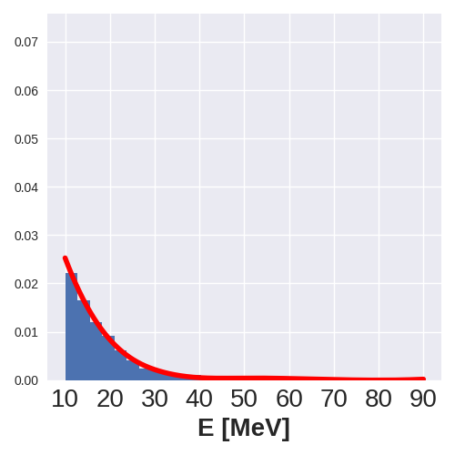 |
|
0 or 1 ntags |
 |
 |
 |
|---|---|---|---|
|
1 ntag |
 |
 |
 |
D.2 Modeling of spallation backgrounds
To model the spallation background PDF we vary the isotope composition of the background as described in Equation 3 and take the nominal spectrum as the average between the two extreme slopes. We parameterize this average by the following function:
| (27) |
where is a normalization factor and are determined by a fit and depend on the SK phase considered. Then, as described in Section VII.3.2, we both vary the isotope composition of the spallation spectrum and distort it to account for energy scale and resolution uncertainties. We then fit the resulting extreme spectra by the function from Equation 27 times a third order polynomial:
| (28) |
and thus parameterize the 1 systematic error distorsions. The nominal spectrum and its associated analytical fit are shown in Fig. 37 for SK-IV with its 1 uncertainty range. Note that, in order to account for the steepness of the spallation spectrum while avoiding unphysical results, we impose for energies larger than the minimal for which the distorted PDF is zero.

References
- Fukugita et al. (1994) M. Fukugita et al., Springer ISBN 978-4-431-67029-2 (1994).
- Kotake et al. (2006) K. Kotake et al., Reports on Progress in Physics 69, 971 (2006).
- Nakazato et al. (2013) K. Nakazato et al., The Astrophysical Journal Supplement Series 205, 2 (2013).
- Tammann et al. (1994) G. Tammann et al., The Astrophysical Journal Supplement 92, 487 (1994).
- Diehl et al. (2006) R. Diehl et al., Nature 439, 45 (2006).
- Nakazato et al. (2015) K. Nakazato et al., The Astrophysical Journal 804, 75 (2015).
- Malaney (1997) R. A. Malaney, Astroparticle Physics 7, 125 (1997).
- Totani and Sato (1995) T. Totani and K. Sato, Astroparticle Physics 3, 367 (1995).
- Kaplinghat et al. (2000) M. Kaplinghat et al., Physical Review D 62, 043001 (2000).
- Lunardini (2009) C. Lunardini, Physical Review Letters 102, 231101 (2009).
- Horiuchi et al. (2018) S. Horiuchi et al., Monthly Notices of the Royal Astronomical Society 475 (2018).
- Kresse et al. (2021) D. Kresse et al., The Astrophysical Journal 909, 2 (2021).
- Horiuchi et al. (2021) S. Horiuchi et al., Physical Review D 103, 043003 (2021).
- Tabrizi and Horiuchi (2021) Z. Tabrizi and S. Horiuchi, Journal of Cosmology and Astroparticle Physics 2021, 05 (2021).
- Galais et al. (2010) S. Galais et al., Physical Review D 81, 053002 (2010).
- Horiuchi et al. (2009) S. Horiuchi et al., Physical Review D 79, 083013 (2009).
- Ando et al. (2003) S. Ando et al., Astroparticle Physics 18, 307 (2003).
- Hartmann and Woosley (1997) D. H. Hartmann and S. E. Woosley, Astroparticle Physics 7, 137 (1997).
- bib (2005) Next Generation of Nucleon Decay and Neutrino Detectors: Proceedings, Aussois, Savoie, France, 7-9 April 2005 (2005).
- Cokinos and Melkonian (1977) D. Cokinos and E. Melkonian, Physical Review C 15, 1636 (1977).
- Malek et al. (2003) M. Malek et al. (Super-Kamiokande Collaboration), Physical Review Letters 90, 061101 (2003).
- Bays et al. (2012) K. Bays et al. (Super-Kamiokande Collaboration), Physical Review D 85, 052007 (2012).
- Zhang et al. (2015) H. Zhang et al. (Super-Kamiokande Collaboration), Astroparticle Physics 60, 41 (2015).
- Gando et al. (2012) A. Gando et al. (KamLAND Collaboration), The Astrophysical Journal 745 (2012).
- Abe et al. (2021a) S. Abe et al. (KamLAND Collaboration), arXiv:2108.08527 [astro-ph.HE] (2021a).
- Aharmim et al. (2006) B. Aharmim et al. (SNO Collaboration), The Astrophysical Journal 653 (2006).
- Aharmim et al. (2020) B. Aharmim et al. (SNO Collaboration), Physical Review D 102, 062006 (2020).
- Agostini et al. (2021) M. Agostini et al. (Borexino Collaboration), Astroparticle Physics 125, 102509 (2021).
- Fukuda et al. (2003) S. Fukuda et al. (Super-Kamiokande Collaboration), Nuclear Instruments and Methods in Physics Research, Section A 501, 418 (2003).
- Kume et al. (1983) H. Kume et al., Nuclear Instruments and Methods in Physics Research, Section A 205 (1983).
- Abe et al. (2014a) K. Abe et al. (Super-Kamiokande Collaboration), Nuclear Instruments and Methods in Physics Research, Section A 737, 253 (2014a).
- Nakahata et al. (1999) M. Nakahata et al. (Super-Kamiokande Collaboration), Nuclear Instruments and Methods in Physics Research, Section A 421, 113 (1999).
- Blaufuss et al. (2001) E. Blaufuss et al. (Super-Kamiokande Collaboration), Nuclear Instruments and Methods in Physics Research, Section A 458, 638 (2001).
- Nishino et al. (2009) H. Nishino et al., Nuclear Instruments and Methods in Physics Research, Section A 610, 710 (2009).
- Watanabe et al. (2009) H. Watanabe et al. (Super-Kamiokande Collaboration), Astroparticle Physics 31, 320 (2009).
- Hosaka et al. (2006) J. Hosaka et al. (Super-Kamiokande Collaboration), Physical Review D 73, 112001 (2006).
- Cravens et al. (2008) J. Cravens et al. (Super-Kamiokande Collaboration), Physical Review D 78, 032002 (2008).
- Abe et al. (2011) K. Abe et al. (Super-Kamiokande Collaboration), Physical Review D 83, 052010 (2011).
- Abe et al. (2016) K. Abe et al. (Super-Kamiokande Collaboration), Physical Review D 94, 052010 (2016).
- Smy (2008) M. Smy, Proceedings of the 30th International Cosmic Ray Conference 5, 1279 (2008).
- Salpeter (1955) E. E. Salpeter, The Astrophysical Journal 121, 161 (1955).
- Keil et al. (2003) M. T. Keil et al., The Astrophysical Journal 590, 971 (2003).
- Strumia and Vissani (2003) A. Strumia and F. Vissani, Physics Letters B 564 (2003).
- Brun et al. (1994) R. Brun et al., Report No. CERN-W5013 (1994).
- Ankowski et al. (2012) A. Ankowski et al., Physical Review Letters 108, 052505 (2012).
- Abe et al. (2014b) K. Abe et al. (T2K Collaboration), Physical Review D 90, 072012 (2014b).
- Wan et al. (2019) L. Wan et al. (Super-Kamiokande Collaboration), Physical Review D 99, 032005 (2019).
- Abe et al. (2019) K. Abe et al. (T2K Collaboration), Physical Review D 100, 112009 (2019).
- Honda et al. (2007) M. Honda et al., Physical Review D 75, 043006 (2007).
- Honda et al. (2011) M. Honda et al., Physical Review D 83, 123001 (2011).
- bib (Flux) http://www.icrr.u-tokyo.ac.jp/~mhonda/nflx2011/index.html (HKKM2011 Flux).
- Hayato (2009) Y. Hayato, Acta Physica Polonica B 40, 2477 (2009).
- Abe et al. (2020) K. Abe et al. (Super-Kamiokande Collaboration), arXiv:2012.03807 [hep-ex] (2020).
- Jiang et al. (2019) M. Jiang et al. (Super-Kamiokande Collaboration), Progress of Theoretical and Experimental Physics 2019, 053F01 (2019).
- Battistoni et al. (2007) G. Battistoni et al., AIP Conference Proceedings 896, 31 (2007).
- Li and Beacom (2014) S. W. Li and J. Beacom, Physical Review C 89, 045801 (2014).
- Li and Beacom (2015a) S. W. Li and J. Beacom, Physical Review D 91, 105005 (2015a).
- Li and Beacom (2015b) S. W. Li and J. Beacom, Physical Review D 92, 105033 (2015b).
- Zhang et al. (2016) Y. Zhang et al. (Super-Kamiokande Collaboration), Physical Review D 93, 012004 (2016).
- bib (eact) https://github.com/Goldie643/SKReact (SKReact).
- Baldoncini et al. (2015) M. Baldoncini et al., Physical Review D 91, 065002 (2015).
- int (2005) Technical Reports Series No. 428 (International Atomic Energy Agency, Vienna, 2005).
- An et al. (2017) F. P. An et al. (Daya Bay), Chin. Phys. C 41, 013002 (2017), arXiv:1607.05378 [hep-ex] .
- Locke et al. (2021) S. M. Locke et al. (Super-Kamiokande Collaboration), to appear (2021).
- Carminati (2011) G. Carminati, in 32nd International Cosmic Ray Conference (2011).
- Carminati (2015) G. Carminati (Super-Kamiokande collaboration), Physics Procedia 61, 666 (2015).
- Elnimr (2017) M. Elnimr (Super-Kamiokande collaboration), Journal of Physics Conference Series. 888, 012189 (2017).
- Conner (1997) Z. Conner, Ph.D Thesis, Boston University (1997).
- Desai (2004) S. Desai, Ph.D Thesis, Boston University (2004).
- Abe et al. (2017) K. Abe et al. (T2K Collaboration), Physical Review D 96, 092006 (2017).
- Zhang (2012) H. Zhang, Ph.D Thesis, Tsinghua University (2012).
- Zhang (2015) Y. Zhang, Ph.D Thesis, Tsinghua University (2015).
- Nakano et al. (2020) Y. Nakano et al., Nuclear Instruments and Methods in Physics Research, Section A 977, 164297 (2020).
- Chen and Guestrin (2016) T. Chen and C. Guestrin, in Proceedings of the 22nd ACM SIGKDD International Conference on Knowledge Discovery and Data Mining, KDD ’16 (ACM, New York, NY, USA, 2016) pp. 785–794.
- Akutsu (2019) R. Akutsu, Ph.D Thesis, The University of Tokyo (2019).
- Abe et al. (2021b) K. Abe et al. (Super-Kamiokande Collaboration), to appear (2021b).
- Abe et al. (2021c) K. Abe et al. (Super-Kamiokande Collaboration), to appear (2021c).
- Rolke et al. (2005) W. A. Rolke et al., Nuclear Instruments and Methods in Physics Research, Section A 551, 493 (2005).
- Benhar et al. (1994) O. Benhar et al., Nuclear Physics A 579, 493 (1994).
- Benhar et al. (2005) O. Benhar et al., Physical Review D 72, 053005 (2005).
- Horowitz and Serot (1981) C. J. Horowitz and B. D. Serot, Nuclear Physics A 368, 503 (1981).
- Maieron et al. (2003) C. Maieron et al., Physical Review C 68, 048501 (2003).
- Caballero et al. (2005) J. A. Caballero et al., Physical Review Letters 95, 252502 (2005).
- Gonzalez-Jimenez et al. (2013) R. Gonzalez-Jimenez et al., Physical Review C 88, 025502 (2013).
- Amaro et al. (2005) J. E. Amaro et al., Physical Review C 71, 015501 (2005).
- Amaro et al. (2006) J. E. Amaro et al., Physical Review C 73, 035503 (2006).
- Capuzzi et al. (1991) F. Capuzzi et al., Nuclear Physics A 524, 681 (1991).
- Meucci et al. (2004) A. Meucci et al., Nuclear Physics A 739, 277 (2004).
- Meucci and Giusti (2014) A. Meucci and C. Giusti, Physical Review D 89, 057302 (2014).
- Ashie et al. (2005) Y. Ashie et al. (Super-Kamiokande Collaboration), Physical Review D 71, 112005 (2005).
- Regis et al. (2012) C. Regis et al. (Super-Kamiokande), Physical Review D 86, 012006 (2012).
- Winter et al. (2006) W. T. Winter et al., Physical Review C 73, 025503 (2006).
- Jegerlehner et al. (1996) B. Jegerlehner et al., Physical Review D 54, 1194 (1996).
- Sisti (2020) M. Sisti (JUNO Collaboration), Journal of Physics Conference Series 1468, 012150 (2020).
- Møller et al. (2018) K. Møller, A. M. Suliga, I. Tamborra, and P. B. Denton, Journal of Cosmology and Astroparticle Physics 05, 066 (2018).