Differentially Private Simple Linear Regression

In this paper we consider the most common model of linear regression: one-dimensional linear regression with homoscedastic noise. This model is defined by a slope $\alpha\in\mathbb{R}$, an intercept $\beta\in\mathbb{R}$, a noise distribution $F_{e}$ with mean $0$ and variance $\sigma_{e}^{2}$, and the relationship

where $\textbf{x},\textbf{y}\in\mathbb{R}^{n}$. Our data consists of $n$ pairs, $(x_{i},y_{i})$, where $x_{i}$ is the explanatory variable, $y_{i}$ is the response variable, and each random variable $e_{i}$ is draw i.i.d. from the distribution $F_{e}$. The goal of simple linear regression is to estimate $\alpha$ and $\beta$ given the data $\{(x_{1},y_{1}),\cdots,(x_{n},y_{n})\}$.

Let $\textbf{x}=(x_{1},\ldots,x_{n})^{T}$, $\textbf{y}=(y_{1},\ldots,y_{n})^{T}$. The Ordinary Least Squares (OLS) solution to the simple linear regression problem is the solution to the following optimization problem:

It is the most commonly used solution in practice since it is the maximum likelihood estimator when $F_{e}$ is Gaussian, and it has a closed form solution. We define the following empirical quantities:

Then

this paper, we focus on predicting the (mean of the) response variable $y$ at a single value of the explanatory variable $x$. For $x_{new}\in[0,1]$, the prediction at $x_{new}$ is defined as:

Let $\widehat{p}_{x_{new}}$ be the estimate of the prediction at $x_{new}$ computed using the OLS estimates $\hat{\alpha}$ and $\hat{\beta}$. The quantity $\widehat{p}_{x_{new}}$ is a random variable, where the randomness is due to the sampling process. The standard error $\widehat{\sigma}(\widehat{p}_{x_{new}})$ is an estimate of the standard deviation of $\widehat{p}_{x_{new}}$. If we assume that the noise $F_{e}$ is Gaussian, then we can compute the standard error as follows (see (Yan and Su, 2009), for example):

It can be shown that the variance of $(\widehat{p}_{x_{new}}-p_{x_{new}})/\widehat{\sigma}(\widehat{p}_{x_{new}})$ approaches $1$ as $n$ increases.

In this section, we define the notion of privacy that we are using: differential privacy (DP). Since our algorithms often include hyperparameters, we include a definition of DP for algorithms that take as input not only the dataset, but also the desired privacy parameters and any required hyperparameters. Let $\mathcal{X}$ be a data universe and $\mathcal{X}^{n}$ be the space of datasets. Two datasets $d,d^{\prime}\in\mathcal{X}^{n}$ are neighboring, denoted $d\sim d^{\prime}$, if they differ on a single record. Let $\mathcal{H}$ be a hyperparameter space and $\mathcal{Y}$ be an output space.

For strong privacy guarantees, the privacy-loss parameter is typically taken to be a small constant less than $1$ (note that $e^{\varepsilon}\approx 1+\varepsilon$ as $\varepsilon\rightarrow 0$), but we will sometimes consider larger constants such as $\varepsilon=8$ to match our motivating application (described in Section 1.2).

The key intuition for this definition is that the distribution of outputs on input dataset $d$ is almost indistinguishable from the distribution on outputs on input dataset $d^{\prime}$. Therefore, given the output of a differentially private mechanism, it is impossible to confidently determine whether the input dataset was $d$ or $d^{\prime}$.

The DP estimates will be denoted by $\widetilde{p}_{x_{new}}$ and the OLS estimates by $\widehat{p}_{x_{new}}$. We will focus on data with values bounded between 0 and 1, so $0\leq x_{i},y_{i}\leq 1$ for $i=1,\ldots,n$.

We will be primarily concerned with the predicted values at $x_{new}=0.25$ and $0.75$, which for ease of notation we denote as $p_{25}$ and $p_{75}$, respectively. Correspondingly, we will use $\widehat{p}_{25},\widehat{p}_{75}$ to denote the OLS estimates of the predicted values and $\widetilde{p}_{25},\widetilde{p}_{75}$ to denote the DP estimates. Our use of the 25th and 75th percentiles is motivated by the Opportunity Atlas tool (Chetty et al., 2018), described in Section 1.2, which releases estimates of $p_{25}$ and $p_{75}$ for certain regressions done for every census tract in each state.

We will be concerned primarily with empirical performance measures. In particular, we will restrict our focus to high probability error bounds that can be accurately computed empirically through Monte Carlo experiments. The question of providing tight theoretical error bounds for DP linear regression is an important one, which we leave to future work. Since the relationship between the OLS estimate $\widehat{p}_{x_{new}}$ and the true value $p_{x_{new}}$ is well-understood, we focus on measuring the difference between the private estimate $\widetilde{p}_{x_{new}}$ and $\widehat{p}_{x_{new}}$, which is something we can measure experimentally on real datasets. Specifically, we define the prediction error at $x_{new}$ to be $|\widetilde{p}_{x_{new}}-\widehat{p}_{x_{new}}|.$

For a dataset $d$, $x_{new}\in[0,1]$, and $q\in[0,100]$, we define the $q\%$ error bound as

where the dataset $d$ is fixed, and the probability is taken over the randomness in the DP algorithm.

We empirically estimate $C(q)$ by running many trials of the algorithm on the same dataset $d$:

We term $\hat{C}(q)(d)$ the $q\%$ empirical error bound. We will often drop the reference to $d$ from the notation. This error metric only accounts for the randomness in the algorithm, not the sampling error.

When the ground truth is known (eg. for synthetically generated data), we can compute error bounds compared to the ground truth, rather than to the non-private OLS estimate. So, let $C_{\text{true}}(q)(d)$ and $\hat{C}_{\text{true}}(q)(d)$ be similar to the error bounds described earlier, except that the prediction error is measured as $|\widetilde{p}_{x_{new}}-p_{x_{new}}|$. This error metric accounts for the randomness in both the sampling and the algorithm. When we say the noise added for privacy is less than the sampling error, we are referring to the technical statement that $\hat{C}(68)$ is less than the standard error, $\widehat{\sigma}(\widehat{p}_{x_{new}})$.

The first differentially private algorithm for the median that we will consider is an instantiation of the exponential mechanism (McSherry and Talwar, 2007), a differentially private algorithm designed for general optimization problems. The exponential mechanism is defined with respect to a utility function $u$, which maps (dataset, output) pairs to real values. For a dataset z, the mechanism aims to output a value $r$ that maximizes $u(\textbf{z},r)$.

One way to instantiate the exponential mechanism to compute the median is by using the following utility function. Let

where #above $r$ and #below $r$ denote the number of datapoints in z that are above and below $r$ in value respectively, not including $r$ itself. An example of the shape of the output distribution of this algorithm is given in Figure 1. An efficient implementation is given in the Appendix.

We will write DPExpTheilSenkMatch to refer to DPTheilSenkMatch where DPmed is the DP exponential mechanism described above with privacy parameter $\varepsilon/k$. Again, we write DPExpTheilSenMatch when $k=1$ and DPExpTheilSen when $k=n-1$.

When the output space is the real line, the standard exponential mechanism for the median has some nuanced behaviour when the data is highly concentrated. For example, imagine in Figure 1 if all the datapoints coincided. In this instance, DPExpTheilSen is simply the uniform distribution on $[r_{l},r_{u}]$, despite the fact that the median of the dataset is very stable. To mitigate this issue, we use a variation on the standard utility function. For a widening parameter $\theta>0$, the widened utility function is

where #above $a$ and #below $a$ are defined as before. This has the effect of increasing the probability mass around the median, as shown in Figure 2.

The parameter $\theta$ needs to be carefully chosen. All outputs within $\theta$ of the median are given the same utility score, so $\theta$ represents a lower bound on the error. Conversely, choosing $\theta$ too small may result in the area around the median not being given sufficient weight in the sampled distribution. Note that $\theta>0$ is only required when one expects the datasets $\textbf{z}^{p25}$ to be highly concentrated (for example when the dataset has strong linear signal). We defer the question of optimally choosing $\theta$ to future work.

An efficient implementation of the $\theta$-widened exponential mechanism for the median can be found in the Appendix as Algorithm 4. We will use DPWideTheilSenkMatch to refer to DPTheilSenkMatch where DPmed is the $\theta$-widened exponential mechanism with privacy parameter $\varepsilon/k$. Again, we use
DPWideTheilSenMatch when $k=1$ and DPWideTheilSen when $k=n-1$.

The final algorithm we consider for releasing a differentially private median adds noise scaled to the smooth sensitivity – a smooth upper bound on the local sensitivity function. Intuitively, this algorithm should perform well when the datapoints are clustered around the median; that is, when the median is very stable.

Let $\mathcal{Z}_{k}:([0,1]\times[0,1])^{n}\rightarrow{\mathbb{R}}^{kn/2}$ to denote the function that transforms a set of point coordinates into estimates for each pair of points in our $k$ matchings, so in the notation of Algorithm 2, $\textbf{z}^{p25}=\mathcal{Z}(\textbf{x},\textbf{y})$. The function that we are concerned with the smooth sensitivity of is med$\circ\mathcal{Z}_{k}$, which maps $(\textbf{x},\textbf{y})$ to med$(\textbf{z}^{p25})$. We will use the following smooth upper bound to the local sensitivity:

The algorithm then adds noise proportional to $S_{\text{med}\circ\mathcal{Z},t}^{k}((\textbf{x},\textbf{y}))/\varepsilon$ to med$\circ\mathcal{Z}(\textbf{x},\textbf{y})$. A further discussion of the formula $S_{\text{med}\circ\mathcal{Z},t}^{k}((\textbf{x},\textbf{y}))$ and pesudo-code can be found in Appendix E. The noise is sampled from the Student’s T distribution. There are several other valid choices of noise distributions (see (Nissim et al., 2007) and (Bun and Steinke, 2019)), but we found the Student’s T distribution to be preferable as the mechanism remains stable across values of $\varepsilon$

The first dataset we consider is a simulated version of the data used by the Opportunity Insights team in creating the Opportunity Atlas tool described in Section 1.2. In the appendix, we describe the data generation process used by the Opportunity Insights team to generate the simulated data. Each datapoint, $(x_{i},y_{i})$, corresponds to a pair, (parent income percentile rank, child income percentile rank) , where parent income is defined as the total pre-tax income at the household level, averaged over the years 1994-2000, and child income is defined as the total pre-tax income at the individual level, averaged over the years 2014-2015 when the children are between the ages of 31-37. In the Census data, every state in the United States is partitioned into small neighborhood-level blocks called tracts. We perform the linear regression on each tract individually. The “best” differentially private algorithm differs from state to state, and even tract to tract. We focus on results for Illinois (IL) which has a total of $n=219,594$ datapoints divided among 3,108 tracts. The individual datasets (corresponding to tracts in the Census data) each contain between $n=30$ and $n=400$ datapoints. The statistic $n\text{var}(\textbf{x})$ ranges between 0 and 25, with the majority of tracts having $n\text{var}(\textbf{x})\in[0,5]$. We use $\varepsilon=16$ in all our experiments on this data since that is the value approved by the Census for, and currently used in, the release of the Opportunity Atlas (Chetty et al., 2018).

Next, we consider a family of small datasets containing data from the Capital Bikeshare system, in Washington D.C., USA, from the years 2011 and 2012¹¹1This data is publicly available at http://capitalbikeshare.com/system-data (Fanaee-T and Gama, 2013).. Each $(x_{i},y_{i})$ datapoint of the dataset contains the temperature ($x_{i}$) and user count of the bikeshare program ($y_{i}$) for a single hour in 2011 or 2012. The $x_{i}$ and $y_{i}$ values are both normalized so that they lie between 0 and 1 by a linear rescaling of the data. In order to obtain smaller datasets to work with, we segment this dataset into 288 (12x24) smaller datasets each corresponding to a (month, hour of the day) pair. Each smaller dataset contains between $n=45$ and $n=62$ datapoints. We linearly regress the number of active users of the bikeshare program on the temperature. While the variables are positively correlated, the correlation is not obviously linear — in that the data is not necessarily well fit by a line — within many of these datasets, so we see reasonably large standard error values ranging between 0.0003 and 0.32 for this data. Note that our privacy guarantee is at the level of hours rather than individuals so it serves more as an example to evaluate the utility of our methods, rather than a real privacy application. While this is an important distinction to make for deployment of differential privacy, we will not dwell on it here since our goal to evaluate the statistical utility of our algorithms on real datasets. An example of one of these datasets is displayed in Figure 3.

While we are primarily concerned with evaluating the behavior of the private algorithms on small datasets, we also present results on a good candidate for private analysis: a large dataset with a strong linear relationship. In contrast to the Bikeshare UCI data and the Opportunity Insights data, this is a single dataset, rather than a family of datasets. This data is drawn from a dataset studying atomic coordinates in carbon nanotubes (Aci and Avci, 2016). For each datapoint $(x_{i},y_{i})$, $x_{i}$ is the $u$-coordinate of the initial atomic coordinates of a molecule and $y_{i}$ is the $u$-coordinate of the calculated atomic coordinates after the energy of the system has been minimized. After we filtered out all points that are not contained in $[0,1]\times[0,1]$, the resulting dataset contains $n=10,683$ datapoints. A graphical representation of the data is included in Figure 4. Due to the size of this dataset, we run the efficient DPTheilSenMatch algorithm with $k=1$ on this dataset. This dataset does not contain sensitive information, however we have included it to evaluate the behaviour of the DP algorithms on a variety of real datasets.

Our final real dataset studies the relationship between the Istanbul Stock Exchange and the USD Stock Exchange (Akb, 2013). ²²2This dataset was collected from imkb.gov.tr and finance.yahoo.com. It compares {$x_{i}=$ Istanbul Stock Exchange national 100 index} to {$y_{i}=$ the USD International Securities Exchange}. This dataset has $n=250$ datapoints and a representation is included in Figure 5. This is a a smaller, noisier dataset than the Carbon Nanotubes UCI dataset.

The synthetic datasets were constructed by sampling $x_{i}\in\mathbb{R}$, for $i=1,\ldots,n$, independently from a uniform distribution with $\bar{x}=0.5$ and variance $\sigma_{x}^{2}$. For each $x_{i}$, the corresponding $y_{i}$ is generated as $y_{i}=\alpha x_{i}+\beta+e_{i}$, where $\alpha=0.5,\beta=0.2$, and $e_{i}$ is sampled from $\mathcal{N}(0,\sigma_{e}^{2})$. The $(x_{i},y_{i})$ datapoints are then clipped to the box $[0,1]^{2}$. The DP algorithms estimate the prediction at $x_{new}$ using privacy parameter $\varepsilon$.

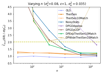
The values of $n$, $\sigma_{x}^{2}$, $\sigma_{e}^{2}$, $x_{new}$, and $\varepsilon$ vary across the individual experiments. The synthetic data experiments are designed to study which properties of the data and privacy regime determine the performance of the private algorithms. Thus, in these experiments, we vary one of parameters listed above and observe the impact on the accuracy of the algorithms and their relative performance to each other. Since we know the ground truth on this synthetically generated data, we plot empirical error bounds that take into account both the sampling error and the error due to the DP algorithms, $\hat{C}_{\text{true}}(68)/\sigma(\widehat{p}_{x_{new}})$. We evaluate DPTheilSenkMatch with $k=10$ in the synthetic experiments rather than DPTheilSen, since the former is computationally more efficient and still gives us insight into the performance of the latter.

In Figure 10, we investigate the relative performance ($\hat{C}_{\text{true}}(68)/\sigma(\widehat{p}_{25})$) of the algorithms in several parameter regimes of $n,\varepsilon$, and $\sigma_{x}^{2}$ on synthetically generated data. For each parameter setting, for each algorithm, we plot of the average value of $\hat{C}_{\text{true}}(68)/\sigma(\widehat{p}_{25})$ over $50$ trials on a single dataset, and average again over $500$ independently sampled datasets. Across large ranges for each of these three parameters ($n\in[30,10,000]$; $\sigma_{x}^{2}\in[0.003,0.03]$; $\varepsilon\in[0.01,10]$, all varied on a logarithmic scale), we see that either DPExpTheilSen, DPGDzCDP, or NoisyStats is consistently the best performing algorithm—or close to it. Note that of these three algorithms, only DPExpTheilSen and NoisyStats fulfill the stronger pure $(\varepsilon,0)$-DP privacy guarantee. We see that DPGDzCDP and NoisyStats trend towards taking over as the best algorithms as $\varepsilon n\sigma_{x}^{2}$ increases.

For parameter regimes in which the non-robust algorithms outperform the robust estimators, NoisyStats is preferable to DPGDzCDP since it is more efficient, requires no hyperparameter tuning (except bounds on the inputs $x_{i}$ and $y_{i}$), fulfills a stronger privacy guarantee, and releases the noisy sufficient statistics with no additional cost in privacy. Experimentally, we find that the main indicator for deciding between robust estimators and non-robust estimators is the quantity $\varepsilon n\text{var}(\textbf{x})$ (which is a proxy for $\varepsilon n\sigma_{x}^{2}$). Roughly, when $\varepsilon n\text{var}(\textbf{x})$ and $\sigma_{e}^{2}$ are both large, NoisyStats is close to optimal among the DP algorithms tested; otherwise, the robust estimator DPExpTheilSen typically has lower error. Hyperparameter tuning and the quantity $|x_{new}-\bar{x}|$ also play minor roles in determining the relative performance of the algorithms.

The quantity $\varepsilon n\text{var}(\textbf{x})$ is related to the size of the dataset, how concentrated the independent variable of the data is and how private the mechanism is. It appears to be a better indicator of the performance of DP mechanisms than any of the individual statistics $\varepsilon,n$, or $\text{var}(\textbf{x})$ in isolation. In Figure 11 we compare the performance of NoisyStats and DPExpTheilSen10Match as we vary $\sigma_{e}^{2}$ and $x_{new}$. For each parameter setting, for each algorithm, the error is computed as the average error over $20$ trials and $500$ independently sampled datasets. Notice that the blue line presents the error of the non-private OLS estimator, which is our baseline. The quantity we control in these experiments is $\varepsilon n\sigma_{x}^{2}$, although we expect this to align closely with $\varepsilon n\text{var}(\textbf{x})$, which is the empirically measurable quantity. In all of our synthetic data experiments, in which the $x_{i}$’s are uniform and the $e_{i}$’s are Gaussian, once $\varepsilon n\sigma_{x}^{2}>400$ and $\sigma_{e}^{2}\geq 10^{-2}$, NoisyStats is close to the best performing algorithm. It is also important to note that once $\varepsilon n\text{var}(\textbf{x})$ is large, both NoisyStats and DPExpTheilSen perform well. See Figure 11 for a demonstration of this on the synthetic data.

The error, as measured by $\hat{C}_{\text{true}}(68)$, of both OLS and Theil-Sen estimators converges to 0 as $n\to\infty$ at the same asymptotic rate. However, OLS converges a constant factor faster than Theil-Sen resulting in its superior performance on relatively large datasets. As $\varepsilon n\text{var}(\textbf{x})$ increases, the error of NoisyStats decreases, and the outputs of this algorithm concentrate around the OLS estimate. While the outputs of DPExpTheilSen tend to be more concentrated, they converge to the Theil-Sen estimate, which has higher sampling error. Thus, as we increase $\varepsilon n\text{var}(\textbf{x})$, eventually the additional noise due to privacy added by NoisyStats is less than the difference between the OLS and Theil-Sen point estimates, resulting in NoisyStats outperforming DPExpTheilSen. This phenomenon can be seen in Figure 10 and Figure 11.

The classifying power of $\varepsilon n\text{var}(\textbf{x})$ is a result of its impact on the performance of NoisyStats. Recall that NoisyStats works by using noisy sufficient statistics within the closed form solution for OLS given in Equation 2. The noisy sufficient statistic $\text{nvar}(\textbf{x})+\text{Lap}(0,3\Delta_{2}/\varepsilon)$, appears in the denominator of this closed form solution. When $\varepsilon n\text{var}(\textbf{x})$ is small, this noisy sufficient statistic has constant mass concentrated near, or below, 0, and hence the inverse, $1/(\text{nvar}(\textbf{x})+\text{Lap}(0,3\Delta_{2}/\varepsilon))$, which appears in the NoisyStats, can be an arbitrarily bad estimate of $1/\text{nvar}(\textbf{x})$. In contrast, when $\varepsilon n\text{var}(\textbf{x})$ is large, the distribution of $\text{nvar}(\textbf{x})+\text{Lap}(0,3\Delta_{2}/\varepsilon)$ is more concentrated around $\text{nvar}(\textbf{x})$, so that with high probability $1/(\text{nvar}(\textbf{x})+\text{Lap}(0,3\Delta_{2}/\varepsilon))$ is close to $1/\text{nvar}(\textbf{x})$.

In Figures 10(a), 10(b) and  10(c), the performance of all the algorithms, including NoisyStats and DPExpTheilSen, are shown as we vary each of the parameters $\varepsilon,n$ and $\sigma_{x}^{2}$, while holding the other variables constant, on synthetic data. In doing so, each of these plots is effectively varying $\varepsilon n\text{var}(\textbf{x})$ as a whole. These plots suggest that all three parameters help determine which algorithm is the most accurate. Figure 11 confirms that $\varepsilon n\text{var}(\textbf{x})$ is a strong indicator of the relative performance of NoisyStats and DPExpTheilSen, even as other variables in the OLS standard error equation (3) – including the variance of the noise of the dependent variable, $\sigma_{e}$, and the difference between $x_{new}$ and the mean of the $x$ values, $|x_{new}-\bar{x}|$ – are varied.

One main advantage that all the DPTheilSen algorithms have over NoisyStats is that they are better able to adapt to the specific dataset. When $\sigma_{e}^{2}$ is small, there is a strong linear signal in the data that the non-private OLS estimator and the DPTheilSen algorithms can leverage. Since the noise addition mechanism of NoisyStats does not leverage this strong signal, its relative performance is worse when $\sigma_{e}^{2}$ is small. Thus, $\sigma_{e}^{2}$ affects the relative performance of the algorithms, even when $\varepsilon n\text{var}(\textbf{x})$ is large. We saw this effect in Figure 9(a) on the Carbon Nanotubes UCI data, where $\varepsilon n\text{var}(x)=889.222$ is large, but NoisyStats performed poorly relative to the DPTheilSen algorithms.

In each of the plots 11(a), 11(c), and 11(e), the quantity $\varepsilon n\text{var}(\textbf{x})$ is held constant while $\sigma_{e}^{2}$ is varied. These plots confirm that the performance of NoisyStats degrades, relative to other algorithms, when $\sigma_{e}^{2}$ is small. As $\sigma_{e}^{2}$ increases, the relative performance of NoisyStats improves until it drops below the relative performance of the TheilSen estimates. The cross-over point varies with $\varepsilon n\text{var}(\textbf{x})$. In Figure 11(a), we see that when $\varepsilon n\text{var}(\textbf{x})$ is small, the methods based on Theil-Sen are the better choice for all values of $\sigma_{e}^{2}$ studied. When we increase $\varepsilon n\text{var}(\textbf{x})$ in Figure 11(e) we see a clear cross over point. These plots add evidence to our conjecture that robust estimators are a good choice when $\varepsilon n\text{var}(\textbf{x})$ and $\sigma_{e}^{2}$ are both small, while non-robust estimators perform well when $\varepsilon n\text{var}\textbf{x}$ is large.