Differential Flatness of Lifting-Wing Quadcopters Subject to Drag and Lift for Accurate Tracking
Abstract
In this paper, we propose an effective unified control law for accurately tracking agile trajectories for lifting-wing quadcopters with different installation angles, which have the capability of vertical takeoff and landing (VTOL) as well as high-speed cruise flight. First, we derive a differential flatness transform for the lifting-wing dynamics with a nonlinear model under coordinated turn condition. To increase the tracking performance on agile trajectories, the proposed controller incorporates the state and input variables calculated from differential flatness as feedforward. In particular, the jerk, the 3-order derivative of the trajectory, is converted into angular velocity as a feedforward item, which significantly improves the system bandwidth. At the same time, feedback and feedforward outputs are combined to deal with external disturbances and model mismatch. The control algorithm has been thoroughly evaluated in the outdoor flight tests, which show that it can achieve accurate trajectory tracking.
SUPPLEMENTARY MATERIAL
Video of the paper summary and experiments is available at https://youtu.be/kj3uOk2P0FQ.
I INTRODUCTION
In recent years, hybrid unmanned aerial vehicles (UAVs) have received extensive attention. These vehicles inherit traditional rotary-wing and fixed-wing aircraft characteristics by compensating for the gravity through rotor-induced thrust and wing-induced lift force. Integrating the advantages of both aircraft, hybrid UAVs have the capability of vertical takeoff and landing (VTOL) as well as high-speed cruise flight.
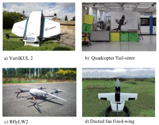
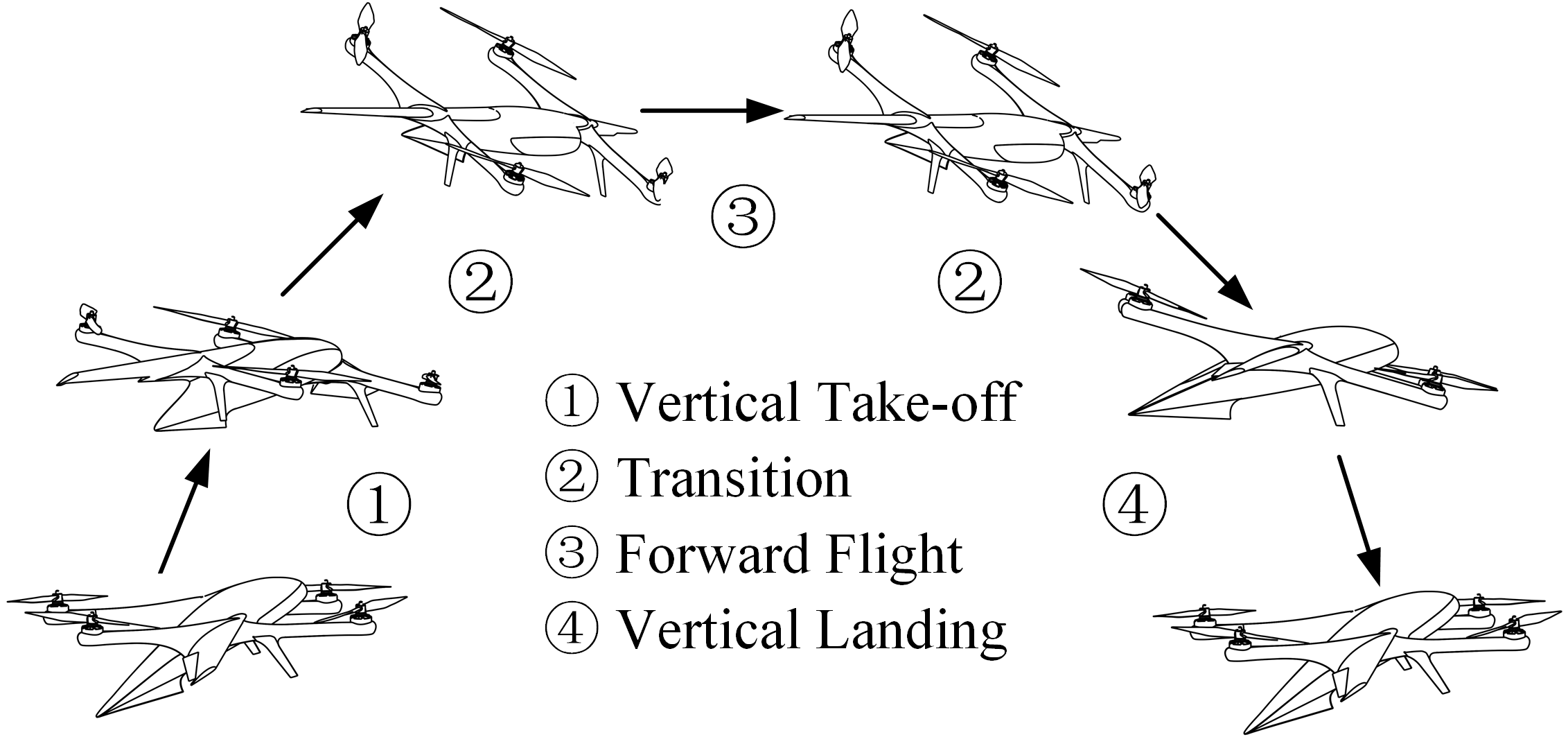
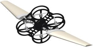
Among the different configurations of hybrid UAVs, there is a type of vehicle with a structure similar to rotary-wing aircraft but with an additional wing, as shown in Fig. 1. The characteristics of this vehicle are that the thrust direction of the rotors is at a fixed angle with the wing, and the aerodynamic interference between the rotor and the wing can be ignored [1] [2]. To achieve horizontal flight, the whole vehicle tilts forward using differential thrust or control vanes, as shown in Fig. 2. We call this type of vehicle lifting-wing quadcopters. They have both the high maneuverability of traditional quadcopters and the long flight range of fixed-wing planes [1][3].
Due to the underactuated property, in trajectory tracking tasks, the lifting-wing quadcopter needs to adjust its attitude to change the direction of collective thrust like quadcopters, so as to obtain the desired acceleration. Because of complex nonlinear aerodynamic forces, the main difficulty in control design is to solve the desired attitude according to the desired acceleration (force mapping) and to make full use of the trajectory information, such as the jerk, to improve the maneuverability of the system. Aimed at these issues, researchers have carried out extensive research.
Compared with traditional quadcopters, the main difference in lifting-wing quadcopters is that they have nonnegligible aerodynamic forces. So, one method is to treat nonlinear aerodynamic forces as unmodeled disturbances. In [4], [5] and [6], aerodynamic forces are modeled offline and directly added to the controller as the feedforward to minimize the model mismatch. Some studies use online estimation methods to compensate for the forces in control, such as adaptive control law [7] and iterative learning method [8] [9] . In [10], a nonlinear optimization algorithm is used to solve the force mapping problem. However, the solver is usually too slow for real-time implementation, because the problem is nonconvex due to the complex aerodynamic model. To improve the real-time performance of the algorithm, a recurrent neural network (RNN) is trained to approximate the behavior of the nonlinear solver [11].
Some researchers try to solve the force mapping problem and maneuverability by utilizing the differential flatness of aircraft, whose state variables and control inputs can be written as algebraic functions of flat outputs and a finite number of their time-derivatives [12]. Using the differential flatness property, a reference trajectory generated in the flat output space can be transformed into the state-control space as feedforward terms. This has been demonstrated to improve trajectory tracking performance in agile flight [13] and trajectory generation efficiency [14] for quadcopters. Only a few attempts have been made to develop the differential flatness property of the aircraft with the wing for trajectory tracking. In [15], the fixed-wing aircraft with a coordinated flight model has been shown to have the differential flatness property when thrust is considered input. However, it cannot be directly applied to aircraft with hovering capability. As for hybrid UAVs, differential flatness is derived for the tail-sitter aircraft with a simplified aerodynamics model [16], but requires an estimate of the aircraft’s lateral aerodynamic force, which is often unavailable.
In this paper, we derive a differential flatness transform for lifting-wing quadcopters subjected to drag and lift, when thrust and angular velocity are considered inputs, so that the force mapping problem is solved. Then, in order to accurately track the agile trajectory, we propose a unified control law, which incorporates the state and input variables calculated from differential flatness as feedforward. In particular, the jerk, the 3-order derivative of the trajectory, is converted into angular velocity as a feedforward item, which significantly improves the system bandwidth. Finally, we verified our algorithm through sufficient outdoor flight experiments, and the flight speed reached up to 10 m/s.
The remainder of this paper is organized as follows: In Section II, we elaborate on the aircraft dynamics with the aerodynamics model in the established coordinate system. Then, in Section III, we derive a differential flatness transform to compute the attitude, thrust and angular velocity from the reference trajectory. In Section IV, a controller for trajectory tracking is designed, and experimental results are shown in Section V. Finally, conclusions are given in Section VI.
II Problem Formulation
II-A Coordinate
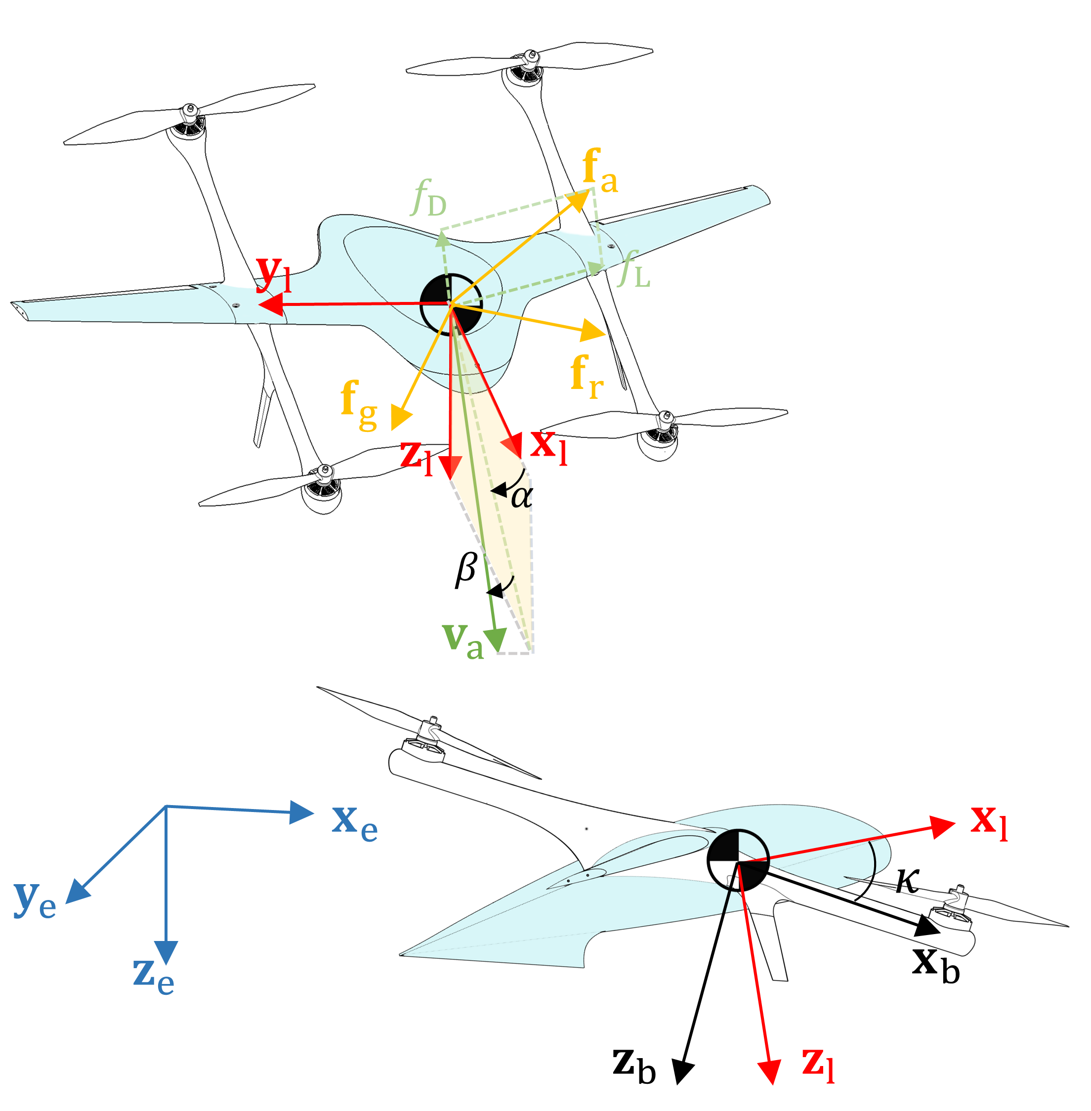
The coordinate frames of the lifting-wing quadcopter are illustrated in Fig. 3. The earth-fixed north-east-down (NED) coordinate , whose basis is composed of the column vectors of the identity matrix , is chosen as the inertial frame. The quadcopter-body coordinate frame is made of an orthonormal basis represented in with the origin located at the center of mass. rotates along by to obtain the lifting-wing coordinate frame , which is made of orthonormal basis represented in . The vector coincides with the chord line and the lifting wing symmetry plane. To handle the wing-induced forces, the wind coordinate frame is defined as with the vector coincides with the airspeed vector . The rotation matrix gives the transformation from (indicated by the subscript b) to (indicated by the superscript e). Throughout this paper, the superscripts are utilized to specify in which coordinate frame a vector is formulated. It should be noted that the superscripts are omitted for vectors in . The position of the lifting-wing quadcopter is denoted as , and its derivatives, velocity, acceleration and jerk as , , , respectively.
II-B Lifting-wing Quadcopter Model
The lifting-wing quadcopter is modeled as a rigid body with six degrees of freedom (6-DOF). The control inputs to the system are taken as the collective thrust and the angular velocity expressed in as . It is assumed that the bandwidth of the angular velocity controller is high enough that the angular dynamics can be neglected. The motion of the aircraft is formulated by Newton and Euler’s Law of Motion [17]:
| (1) | ||||
| (2) | ||||
| (3) |
where is the mass of the aircraft, and denotes the skew-symmetric matrix. In addition, represents forces acting on the airframe expressed in . As shown in Fig. 3, the forces acting on the aircraft are
| (4) |
where with is the collective thrust produced by rotors, is aerodynamic forces produced by the lifting wing, and is the gravitational acceleration vector with .
A special parametric expression is used to model steady aerodynamic forces [18]:
| (5) |
where is the air density, is the surface of the wing. The airspeed vector is defined as , is wind velocity expressed in , is the airspeed, is the angle of attack; aerodynamic parameters is the minimum drag coefficient, is the minimum side force coefficient, is a coefficient related to lift, which are determined by the airfoil. This model is further developed and improved in [19], where a theory method is proposed and demonstrates that the model can cover the main dynamic characteristics in the full flight envelope.
When converted to , is an expression independent of the angle of attack:
| (6) |
Rotation matrix transforms a vector from to given as
| (7) |
where is the installation angle of the lifting wing. In practice applications, different installation angles can be designed according to specific flight indexes, such as flight speed and range. Generally, the installation angle is set at about 45 degrees to ensure good wind resistance [1] [20], as shown in Fig. 1(a) and (c). In particular, when the installation angle is set at 90 degrees, it is the so-called tail-sitter aircraft, as shown in Fig. 1(b) and (d). This type of aircraft is more similar to the fixed wing in cruise flight [2][7]. In this paper, we limit , because when is small, additional propellers are usually added, which is a common dual-system aircraft [21].
II-C Objective
The control design aims to accurately track the trajectory reference . The reference , which is at least 3-order continuous, may be provided by a pre-planned trajectory or an online motion planning algorithm.
To facilitate the problem description, a brief introduction to differential flattening is given. Considering the following dynamic system:
| (8) | ||||
| (9) |
an essential property of flat systems is that their state and input can be directly written as algebraic functions of the flat output and a finite number of its time-derivatives. However, the input and state variables calculated from the flat output cannot be used to directly control the dynamic system (9) because of the inevitable model uncertainty. In practice, they can serve as feedforward control inputs to improve trajectory tracking performance by reducing the phase lag. At the same time, the model uncertainty can be compensated for by the feedback control.
III DIFFERENTIAL FLATNESS
In this section, we show that the dynamics of a lifting-wing quadcopter subject to lift and drag is differentially flat. In fact, the states and inputs can be written as algebraic functions of the flat output and its derivatives. The position , velocity and acceleration can be easily obtained from Eqs (1)-(3). Next, we will derive the reference attitude and thrust from the reference trajectory and its derivatives, and prove how to obtain the reference angular velocity under the coordinated turn condition.
III-A Attitude and Thrust
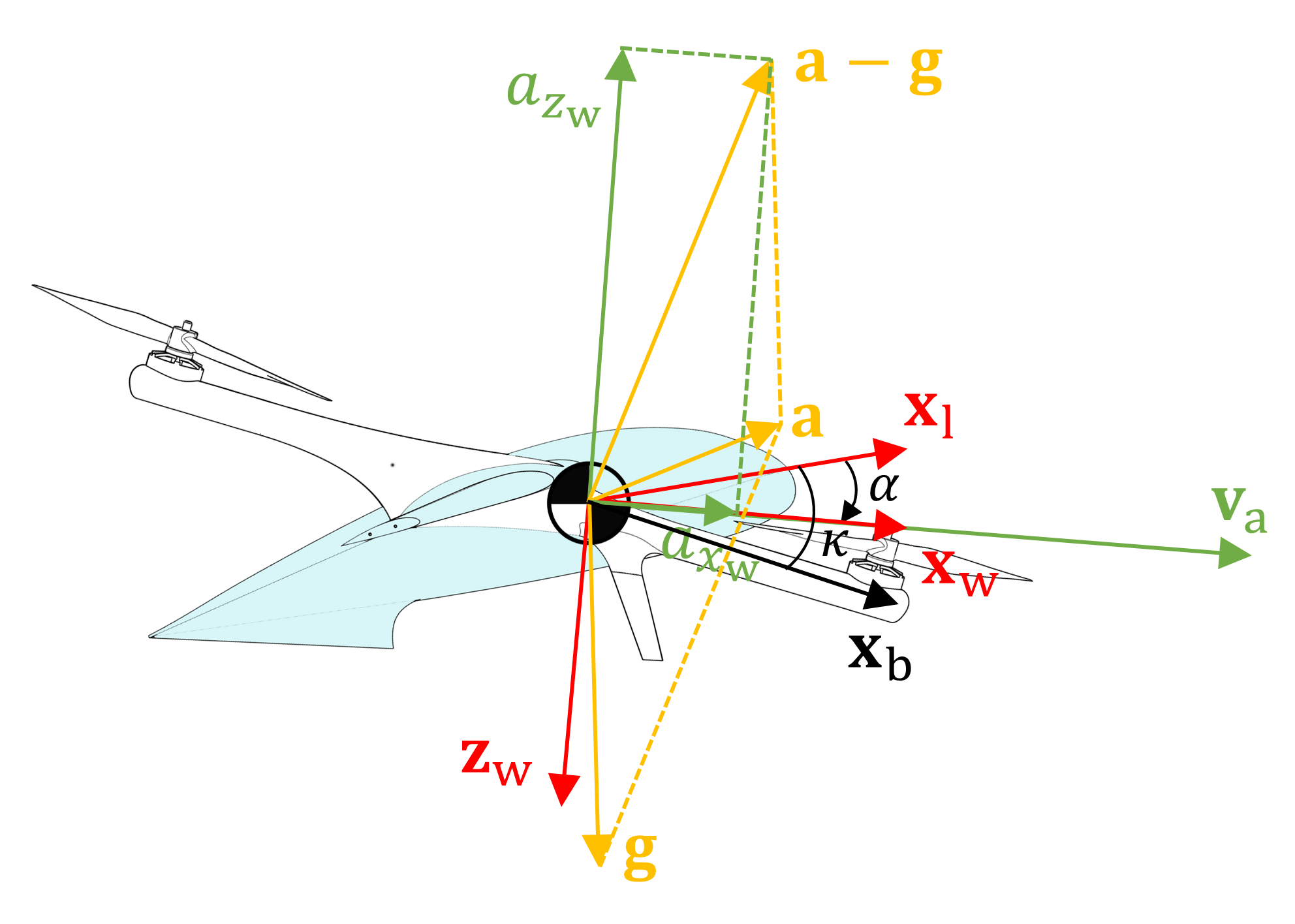
During a coordinated turn, there is no lateral acceleration expressed in of the aircraft, that is , as shown in Fig. 4. Then, the dynamic equation (2) is reformulated as
| (12) |
Since the vector coincides with the airspeed vector, is calculated as
| (13) |
when the wind velocity and the norm of the reference velocity . In fact, if the wind velocity can be estimated online, the results of differential flatness hold true. For the convenience of the following derivation, the wind velocity is assumed to be 0. The case where will be discussed later in section III-C.
Left-multiplying (12) by yields
| (14) |
In , the reference acceleration is constrained in plane. Then, the component of the reference acceleration along can be derived from (12) by substituting (14) and applying the Euclidean norm
| (15) |
Further, considering aerodynamic forces and rotor thrust, the transitional dynamics of the aircraft expressed in are
| (16) |
where and is the transformation from to given by
| (17) |
Substituting (4) and (6) into (2), the position dynamic equation is reformulated as
| (20) |
where , , , , .
Under the coordinated turn condition, can be obtained by rotating along by , which implies that is perpendicular to . With this and (21), is obtained as
| (23) |
According to Rodrigues’ formula, is obtained as
| (24) |
Then, utilizing the orthogonality of rotation matrix, is constructed as
| (25) |
III-B Angular Velocity
Taking the derivative of (20) yields
| (26) |
where
Left-multiplying (26) by yields
| (30) |
Left-multiplying (26) by yields
| (31) |
III-C Special Cases
In this section, we will introduce some practical solutions to solve the special case that the proposed method is invalid.
Case 1 - : For the lifting-wing quadcopter, the case often occurs. For example, when the aircraft is commanded to hover, the reference velocity is desired to be . In fact, when , and are not defined, but this does not mean that and cannot be solved. In Section III-A, we use the wind speed vector to determine the nose orientation of the aircraft, but when the wind speed vector is 0, the nose orientation of the aircraft cannot be determined accordingly. In this case, , originally determined by (23), can be any vector on the plane perpendicular to . To determine the attitude of the aircraft, the yaw angle should be given when , then is obtained as
| (34) |
where .
However, state mutation may occur by directly giving an arbitrary yaw angle. Another simple and effective method is to keep to the last state when is not equal to 0.
Case 2 - : This case occurs if is aligned with , for example when the aircraft needs to execute the vertical takeoff or landing command. In this case, can be any vector on the plane perpendicular to . To overcome this singularity, can be obtained using the same method as in Case 1.
IV CONTROL LAW
To accurately track a reference trajectory, a controller, consisting of feedback terms computed from tracking errors as well as feedforward terms computed from the reference trajectory using the differential flatness property of the lifting-wing quadcopter, is designed. The control architecture consists of an outer-loop position controller and an inner-loop attitude controller. The position controller computes the desired acceleration, which is mapped to the collective thrust and attitude. The attitude command is sent to the inner loop, and the attitude controller generates the desired angular velocity. A high-bandwidth controller is used to track these angular velocity commands and thrust.
IV-A Position and Velocity Controller
Cascaded PID controllers for position (1) and velocity (2) are designed as
| (38) |
| (39) |
where , , are diagonal matrix acting as the feedback control gain. The integral term is added to compensate for model errors and external disturbances. According to the results of Section III, the desired collective thrust and desired attitude can be obtained from . However, in the actual flight, there is the inevitable deviation between the aerodynamic force calculated by (6) and acting on the aircraft. Multiplying the aerodynamic force by an attenuated feedforward coefficient can reduce the adverse effects caused by the inaccurate model. So the desired mass-normalized collective thrust expressed in is obtained as
| (40) |
where are diagonal matrix acting as the feedforward control gain, and is the acceleration due to aerodynamic forces, obtained as
| (41) |
The desired mass-normalized collective thrust is completely produced by rotor thrust, so the desired attitude is obtained as
| (46) |
where is obtained by (13). By projecting the desired acceleration onto the quadcopter-body -axis, the collective thrust input is computed as
| (47) |
IV-B Attitude Controller
The attitude error is presented in the form of quaternion based on which the corresponding controller is designed:
| (48) |
where is transformed from , is the conjugate of a quaternion, and is the quaternion product. Then, is transformed into the axis-angle form by
| (51) |
The function constrains the in to ensure the shortest rotation path. To eliminate the attitude error, the attitude controller is designed as
| (52) |
where is diagonal matrix acting as the control gain.
V REAL-WORLD EXPERIMENTS
In this section, we evaluate the performance of the proposed controller in outdoor scenes, including high-speed and agile circle and lemniscate trajectories.
V-A Experimental Setup
We prepared a lifting-wing quadcopter with a special installation angle for experiments, as shown in Fig. 5. The lifting wing is made of foam and connected to the quadcopter through a 3D-printing connector which controls the installation angle. The power system involves a 3300mAh, four-cell lithium polymer (LiPo) battery, EMAX RS2205 2600KV brushless DC motors with HQ5045 BN propeller, and 45A electronic speed control (ESC). A Pixhawk flight controller111https://docs.px4.io/master/en/assembly/quick_start_pixhawk4.html is rigidly attached to the center of the quadcopter frame, which has an on-board inertial measurement unit (IMU), barometer and SD card for flight data logging. A separate NEO-M8N based GPS module with a magnetometer is used to read the positioning and heading. A Benewake TFmini Lidar with a 40 m range is used for altitude estimation. A 900MHz telemetry link performs communication between the ground control station and the Pixhawk. The flight control algorithm runs on the Pixhawk at 250 Hz.
To validate our theoretical results, we present two trajectories, that is, circle and Lemniscate trajectories, and use the root mean square position error (RMSE) to evaluate the trajectory tracking performance, which is defined as
| (53) |
where is the control cycles of the position controller required to execute a given trajectory.
V-B Circle Trajectory
The circle trajectory is expressed as
| (54) |
where is the local position of the vehicle when the task starts. Here, we set m, rad/s, and when the magnitude of the reference velocity is accelerated to m/s, the system will switch to a circle trajectory with a constant speed.
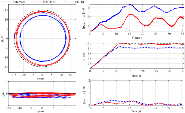
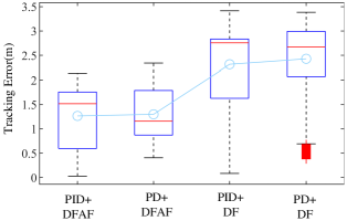
We compare the position error of the lifting-wing quadcopter flying the circle trajectory described above for four conditions: (i) PID velocity controller expressed in (39) with feedforward references computed from the differential flatness transform considering aerodynamic forces (PID+DFAF), (ii) PD velocity controller with feedforward references considering aerodynamic forces (PD+DFAF), (iii) PID velocity controller with feedforward references without considering aerodynamic forces (PID+DF), and (iv) PD velocity controller with feedforward references without considering aerodynamic forces (PD+DF). We have also tried to remove the angular velocity feedforward. As a result, the aircraft deviated significantly from the trajectory when the speed is increased to about 9m/s. Therefore, this flight data is not included in the comparison.
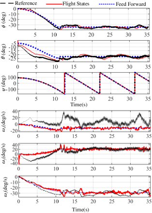
Fig. 6 shows experimental results for tracking a circular trajectory reference on conditions (ii) and (iv). The velocity has a low-frequency sine wave, caused by the state estimator, because the update frequency of GPS is only 10Hz, which brings a considerable delay to the position estimation. The altitude tracking error is far less than that of the horizontal position, because, on the one hand, the Lidar provides higher measurement accuracy than GPS, and on the other hand, the altitude command is constant. The tracking performance statistics for four conditions are summarized in Fig. 7. From these statistics, it can be observed that the trajectory tracking performance has been improved significantly when considering aerodynamic forces and the integral can reduce tracking error, but its effect is very limited. The of conditions (i) and (ii) are about half of that of (iii) and (iv). Fig. 8 shows states of the vehicle agree well with the feedforward commands, demonstrating that the simplified aerodynamic model (6) has fairly good fitting accuracy.
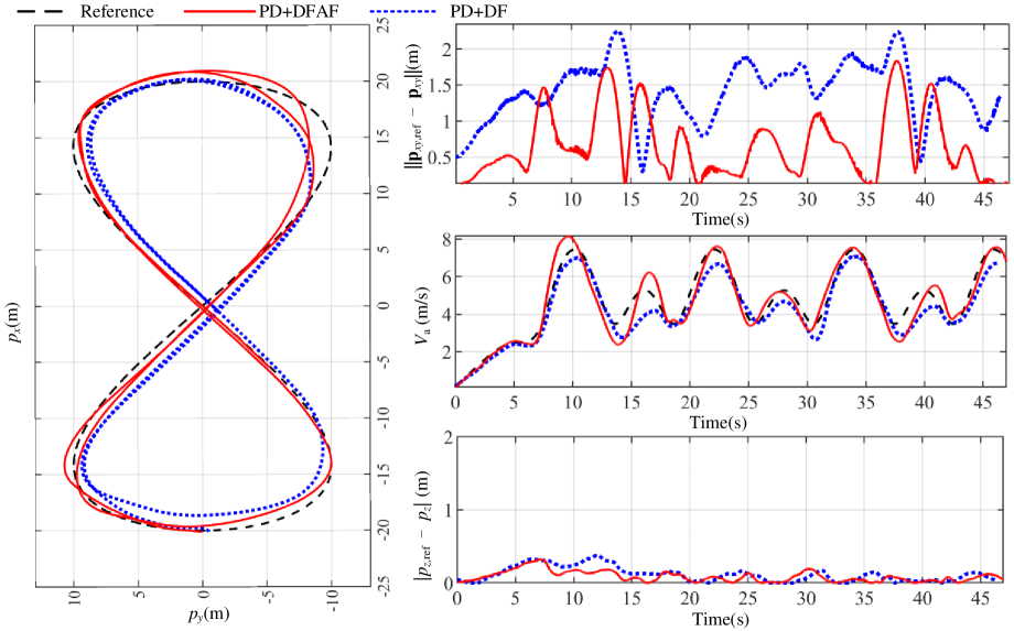
V-C Lemniscate Trajectory
The Lemniscate trajectory is expressed as
| (55) |
Here, we set m, rad/s. Fig. 9 shows experimental results for tracking a Lemniscate of Gerono with an increasing speed from 0 m/s to 8 m/s on conditions (ii) and (iv) with the same aerodynamic coefficients in the circle trajectory. It also can be observed that the trajectory tracking performance has been improved significantly when considering aerodynamic forces, with the reduced by half.
VI CONCLUSION
In this paper, we propose an effective unified control law to track agile trajectories for lifting-wing quadcopters. First, we derive the differential flatness of the lifting-wing quadcopters, which can transform the reference trajectory into the velocity, acceleration, thrust, attitude, and angular velocity commands. Then, the proposed controller combines these feedforward commands and feedback outputs to accurately track agile trajectories. The outdoor experiment results show that the proposed control law can reduce the tracking error by half.
References
- [1] H.-T. Zhang, S. Tan, Z. Song, and Q. Quan, “Performance evaluation and design method of lifting-wing multicopters,” IEEE/ASME Trans. Mechatronics, vol. 27, no. 3, pp. 1606–1616, 2021.
- [2] X. Lyu, J. Zhou, H. Gu, Z. Li, S. Shen, and F. Zhang, “Disturbance observer based hovering control of quadrotor tail-sitter VTOL UAVs using synthesis,” IEEE Robot. Autom. Lett., vol. 3, no. 4, pp. 2910–2917, 2018.
- [3] K. Xiao, Y. Meng, X. Dai, H. Zhang, and Q. Quan, “A lifting wing fixed on multirotor UAVs for long flight ranges,” in Proc. Int. Conf. Unmanned Aircr. Syst., 2021, pp. 1605–1610.
- [4] W. Zhou, B. Li, J. Sun, C.-Y. Wen, and C.-K. Chen, “Position control of a tail-sitter UAV using successive linearization based model predictive control,” Control Eng. Practice, vol. 91, pp. 104–125, 2019.
- [5] W. Xu, H. Gu, Y. Qing, J. Lin, and F. Zhang, “Full attitude control of an efficient quadrotor tail-sitter VTOL UAV with flexible modes,” in Proc. Int. Conf. Unmanned Aircr. Syst., 2019, pp. 542–550.
- [6] F. Zhang, X. Lyu, Y. Wang, H. Gu, and Z. Li, “Modeling and flight control simulation of a quadrotor tailsitter VTOL UAV,” in Proc. AIAA Model. Simul. Technol. Conf., 2017, p. 1561.
- [7] Z.-H. Cheng and H.-L. Pei, “Transition analysis and practical flight control for ducted fan fixed-wing aerial robot: Level path flight mode transition,” IEEE Robot. Autom. Lett., vol. 7, no. 2, pp. 3106–3113, 2022.
- [8] N. Raj, A. Simha, M. Kothari, R. N. Banavar, et al., “Iterative learning based feedforward control for transition of a biplane-quadrotor tailsitter UAS,” in Proc. IEEE Int. Conf. Robot. Autom., 2020, pp. 321–327.
- [9] W. Xu and F. Zhang, “Learning Pugachev’s cobra maneuver for tail-sitter UAVs using acceleration model,” IEEE Robot. Autom. Lett., vol. 5, no. 2, pp. 3452–3459, 2020.
- [10] J. Zhou, X. Lyu, Z. Li, S. Shen, and F. Zhang, “A unified control method for quadrotor tail-sitter UAVs in all flight modes: Hover, transition, and level flight,” in Proc. IEEE/RSJ Int. Conf. Intell. Robots Syst., 2017, pp. 4835–4841.
- [11] J. Zhou, H. Xu, Z. Li, S. Shen, and F. Zhang, “Control of a tail-sitter VTOL UAV based on recurrent neural networks,” arXiv preprint arXiv:2104.02108, 2021.
- [12] M. Fliess, J. Lévine, P. Martin, and P. Rouchon, “Flatness and defect of non-linear systems: introductory theory and examples,” Int. J. Control, vol. 61, no. 6, pp. 1327–1361, 1995.
- [13] M. Faessler, A. Franchi, and D. Scaramuzza, “Differential flatness of quadrotor dynamics subject to rotor drag for accurate tracking of high-speed trajectories,” IEEE Robot. Autom. Lett., vol. 3, no. 2, pp. 620–626, 2017.
- [14] M. W. Mueller, M. Hehn, and R. D’Andrea, “A computationally efficient motion primitive for quadrocopter trajectory generation,” IEEE Trans. Robot., vol. 31, no. 6, pp. 1294–1310, 2015.
- [15] J. Hauser and R. Hindman, “Aggressive flight maneuvers,” in Proc. IEEE Conf. Decision Control, vol. 5, 1997, pp. 4186–4191.
- [16] E. A. Tal and S. Karaman, “Global trajectory-tracking control for a tailsitter flying wing in agile uncoordinated flight,” in AIAA Aviat. Aeronaut. Forum Expos., 2021, p. 3214.
- [17] Q. Quan, Introduction to Multicopter Design and Control. Springer, Singapore, 2017.
- [18] D. Pucci, T. Hamel, P. Morin, and C. Samson, “Nonlinear control of PVTOL vehicles subjected to drag and lift,” in Proc. IEEE Conf. Decision Control, 2011, pp. 6177–6183.
- [19] L. R. Lustosa, F. Defaÿ, and J.-M. Moschetta, “Global singularity-free aerodynamic model for algorithmic flight control of tail sitters,” J. Guid. Control Dyn., vol. 42, no. 2, pp. 303–316, 2019.
- [20] B. Theys, G. De Vos, and J. De Schutter, “A control approach for transitioning VTOL UAVs with continuously varying transition angle and controlled by differential thrust,” in Proc. Int. Conf. Unmanned Aircr. Syst., 2016, pp. 118–125.
- [21] A. S. Saeed, A. B. Younes, S. Islam, J. Dias, L. Seneviratne, and G. Cai, “A review on the platform design, dynamic modeling and control of hybrid UAVs,” in Proc. Int. Conf. Unmanned Aircr. Syst., 2015, pp. 806–815.