Differential equations defined by Kreĭn-Feller operators on Riemannian manifolds

Sze-Man Ngai Beijing Institute of Mathematical Sciences and Applications, Huairou District, 101400, Beijing, China, and Key Laboratory of High Performance Computing and Stochastic Information Processing (HPCSIP) (Ministry of Education of China), College of Mathematics and Statistics, Hunan Normal University, Changsha, Hunan 410081, China. [email protected] and Lei Ouyang Key Laboratory of High Performance Computing and Stochastic Information Processing (HPCSIP) (Ministry of Education of China, College of Mathematics and Statistics, Hunan Normal University, Changsha, Hunan 410081, China. [email protected]

Abstract.

We study linear and semi-linear wave, heat, and Schrödinger equations defined by Kreĭn-Feller operator $-\Delta_{\mu}$ on a complete Riemannian $n$ -manifolds $M$ , where $\mu$ is a finite positive Borel measure on a bounded open subset $\Omega$ of $M$ with support contained in $\overline{\Omega}$ . Under the assumption that $\underline{\operatorname{dim}}_{\infty}(\mu)>n-2$ , we prove that for a linear or semi-linear equation of each of the above three types, there exists a unique weak solution. We study the crucial condition $\dim_{(}\mu)>n-2$ and provide examples of measures on $\mathbb{S}^{2}$ and $\mathbb{T}^{2}$ that satisfy the condition. We also study weak solutions of linear equations of the above three classes by using examples on $\mathbb{S}^{1}$ .

Key words and phrases:

Riemannian manifold; Kreĭn-Feller operator; wave equation; heat equation; Schrödinger equation.

2010 Mathematics Subject Classification:

Primary: 28A80; Secondary: 35D30, 35K05, 35Q41, 35L05.

The authors are supported in part by the National Natural Science Foundation of China, grant 12271156, and Construct Program of the Key Discipline in Hunan Province. The second author was supported in part by Beijing Institute of Mathematical Sciences and Applications (BIMSA)

1. Introduction

The Kreĭn-Feller operator, studied independently by Kreĭn and Feller, is of particular interest in fractal geometry. It is a natural generalization of the Laplace or Laplace-Beltrami operator, and has been applied successfully to study analytic properties of certain fractal measures. Let $\mu$ be a finite positive Borel measure on a bounded open subset $\Omega$ of $\mathbb{R}^{n}$ with support contained in $\overline{\Omega}$ . If $\mu$ satisfies the Poincaré inequality on $\Omega$ , then there exists a Laplacian $\Delta_{\mu}$ defined by $\mu$ . $\Delta_{\mu}$ is also called a Kreĭn-Feller operator (see definition in Section 2) and has been studied extensively in connection with fractal geometry, such as existence of an orthonormal basis of eigenfunctions, spectral dimension and spectral asymptotics, eigenvalues and eigenfunctions, eigenvalue estimates, wave equations and wave speed, heat equation and heat kernel estimates, Schrödinger equation (see [22, 14, 15, 16, 17, 18, 29, 30, 31, 36, 38, 39, 4, 12, 43, 8, 44, 24, 45, 25] and references therein). Chan et al.[8] studied approximations of the solution of the wave equation defined by a one-dimensional fractal Laplacian. Tang and Wang [46] proved the existence and uniqueness of weak solution of the strong damping linear wave equation. Tang and Ngai [45] studied the heat equation on a bounded open set $U\subseteq\mathbb{R}^{n}$ supporting a Borel measure and obtained asymptotic bounds for the solution. For a Schrödinger operator defined by a fractal measure with a continuous potential and a coupling parameter, Ngai and Tang [34] obtained an analog of a semiclassical asymptotic formula for the number of bound states as the parameter tends to infinity. Under the assumption that the Laplacian has compact resolvent, Ngai and Tang [35] proved that there exists a unique weak solution for a linear Schrödinger equation, and obtained the existence and uniqueness of a weak solution of a semi-linear Schrödinger equation.

Fractal phenomena on manifolds have been observed by physicists (see, e.g., [2, 5, 6, 3]); this partly motivated our work. In this paper, we let $M$ be a complete oriented smooth Riemannian $n$ -manifold, let $\Omega\subseteq M$ be a bounded open set, and let $\mu$ be a finite positive Borel measure on $M$ such that ${\rm supp}(\mu)\subseteq\overline{\Omega}$ and $\mu(\Omega)>0$ . Under the assumption $\underline{\operatorname{dim}}_{\infty}(\mu)>n-2$ (see definition in (2.2)) the authors [32, 33] proved that a Kreĭn-Feller operator defined on $M$ has compact resolvent so that there exists an orthonormal basis of $L^{2}(\Omega,\mu)$ consisting of eigenfunctions of $\Delta_{\mu}$ . They also proved the Hodge theorem concerning the eigenvalues and eigenfunctions of the Kreĭn-Feller operator and generalization to the space of differential forms. The first objective of this paper is to study the solution of the following semi-linear wave equation defined by a Kreĭn-Feller operator on $M$ , subject to the specified initial and boundary conditions:

\displaystyle\left\{\begin{array}[]{lll}\partial_{tt}u-\Delta_{\mu}u=F(u)&\text{on}\,\,\,\Omega\times[0,T],\\ u=0&\text{on}\,\,\,\partial\Omega\times[0,T],\\ u=g,\,\,\partial_{t}u=h&\text{on}\,\,\,\Omega\times\{t=0\},\end{array}\right.

(1.4)

where $u:=u(t)$ is an $L^{2}([0,T],\operatorname{dom}\mathcal{E})$ -valued function of $t$ and $F(\cdot)\in{\rm Lip}(\operatorname{dom}\mathcal{E})$ . The notations $\operatorname{dom}\mathcal{E}$ , ${\rm Lip}(\operatorname{dom}\mathcal{E})$ , and $L^{2}([0,T],\operatorname{dom}\mathcal{E})$ are defined in Section 2. Throughout this paper, if $\partial\Omega=\emptyset$ , it is understood that the condition $u=0$ on $\partial\Omega\times[0,T]$ imposes no restriction on the solution. The existence and uniqueness of weak solution of equation (1.4) will be proved in Theorem 3.4.

The second objective of this paper is to study the solution of the following semi-linear heat equation defined by $\Delta_{\mu}$ :

\displaystyle\left\{\begin{array}[]{lll}\partial_{t}u-\Delta_{\mu}u=F(u)&\text{on}\,\,\,\Omega\times[0,T],\\ u=0&\text{on}\,\,\,\partial\Omega\times[0,T],\\ u=g&\text{on}\,\,\,\Omega\times\{t=0\}.\end{array}\right.

(1.8)

The existence and uniqueness of weak solution of this equation will be described in Theorem 4.4.

The third objective of this paper is to study the solution of the following semi-linear Schrödinger equation defined by $\Delta_{\mu}$ :

\displaystyle\left\{\begin{array}[]{lll}i\partial_{t}u+\Delta_{\mu}u=F(u)&\text{on}\,\,\,\Omega\times[0,T],\\ u=0&\text{on}\,\,\,\partial\Omega\times[0,T],\\ u=g&\text{on}\,\,\,\Omega\times\{t=0\}.\end{array}\right.

(1.12)

The existence and uniqueness of weak solution of equation (1.12) will be described in Theorem 5.4.

We also give two classes of measures that satisfy the condition $\underline{\operatorname{dim}}_{\infty}(\mu)>n-2$ . They are the invariant measures $\mu$ of iterated function systems (IFS) on $\mathbb{S}^{2}$ consisting of bi-Lipschitz mappings (Example 6.3), and graph iterated function systems (GIFS) of similitudes on the flat torus $\mathbb{T}^{2}$ (Example 7.6). We also study weak solutions of linear equations of the above three classes by using examples constructed on $\mathbb{S}^{1}$ .

This paper is organized as follows. In Section 2, we summarize some definitions and results that will be needed throughout the paper. The existence and uniqueness of weak solutions of the wave, heat, and Schrödinger equations are studied in Sections 3, 4, and 5, respectively. In Section 6, we give an example of the invariant measures $\mu$ of iterated function systems (IFS) consisting bi-Lipschitz mappings on $\mathbb{S}^{2}$ that satisfy $\underline{\operatorname{dim}}_{\infty}(\mu)>0$ . In Section 7, we give another class of the invariant measures $\mu$ of graph iterated function systems (GIFS) of similitudes on the torus $\mathbb{T}^{2}$ that satisfy $\underline{\operatorname{dim}}_{\infty}(\mu)>0$ . Section 8 illustrates weak solutions of the linear wave, heat, and Schrödinger equations by using examples.

2. Preliminaries

In this section, we summarize some notation, definitions, and preliminary results used throughout the rest of the paper.

2.1. Notation

Definition 2.1.

Let $X$ be a Banach space, $u:(a,b)\subseteq\mathbb{R}\to X$ , and $t_{0}\in(a,b)$ . We say that $u$ is differentiable at $t_{0}$ in the norm $\|\cdot\|_{X}$ if there exists $v_{0}\in X$ such that

\displaystyle\lim_{h\to 0}\Big{\|}\frac{u(t_{0}+h)-u(t_{0})}{h}-v_{0}\Big{\|}_{X}=0.

$v_{0}$ is called the derivative of $u$ at $t_{0}$ , and we write

\displaystyle v_{0}:=\partial_{t}u(t_{0}):=\lim_{h\to 0}\frac{u(t_{0}+h)-u(t_{0})}{h}.

Similarly, the second-order derivative of $u$ at $t_{0}$ denoted $v_{1}$ , is defined as

\displaystyle v_{1}:=\partial_{tt}u(t_{0}):=\lim_{h\to 0}\frac{\partial_{t}u(t_{0}+h)-\partial_{t}u(t_{0})}{h}.

Definition 2.2.

(see [8]) Let $X$ be a separable Banach space with norm $\|\cdot\|_{X}$ . Let $L^{p}([0,T],X)$ be the space of all measurable functions $u:[0,T]\to X$ satisfying

(1)

$\|u\|_{L^{p}([0,T],X)}:=\Big{(}\int_{0}^{T}\|u(t)\|_{X}^{p}\,dt\Big{)}^{1/p}<\infty$ , if $1\leq p<\infty$ , and
(2)

$\|u\|_{L^{\infty}([0,T],X)}:=\mathop{\operatorname{ess\,sup}}\limits_{0\leq t\leq T}\|u(t)\|_{X}<\infty$ , if $p=\infty$ .

When no confusion is possible, we abbreviate these norms as $\|u\|_{p,X}$ and $\|u\|_{\infty,X}$ .

Remark 2.3.

For each $1\leq p\leq\infty$ , $L^{p}([0,T],X)$ is a Banach space. Moreover, if $0\leq p_{1}\leq p_{2}\leq\infty$ , then $L^{p_{1}}([0,T],X)\subseteq L^{p_{2}}([0,T],X)$ . If $(X,\langle\cdot,\cdot\rangle_{X})$ is a separable Hilbert space, then $L^{2}([0,T],X)$ is a Hilbert space with the inner product

\displaystyle\langle u,v\rangle_{L^{2}([0,T],X)}:=\int_{0}^{T}\langle u(t),v(t)\rangle_{X}\,dt

(see, e.g., [1, 47]).

Definition 2.4.

Let $X$ be a Banach space. We define $C([0,T],X)$ as the vector space of all continuous functions $u:[0,T]\to X$ such that

\displaystyle\|u\|_{C([0,T],X)}:=\max_{0\leq t\leq T}\|u(t)\|_{X}<\infty.

Similarly, we define $C^{1}([0,T],X)$ to be the vector space of all continuous differentiable functions $u:[0,T]\to X$ such that

\displaystyle\|u\|_{C^{1}([0,T],X)}:=\max_{0\leq t\leq T}\big{(}\|u(t)\|_{X}+\|\partial_{t}u(t)\|_{X}\big{)}<\infty.

Definition 2.5.

Let $\mathcal{H}$ be a Hilbert space with norm $\|\cdot\|_{\mathcal{H}}$ . We say that a map $F:\mathcal{H}\to\mathcal{H}$ is Lipschitz continuous on $\mathcal{H}$ if there exists some constant $c>0$ such that

\displaystyle\|F(u)-F(v)\|_{\mathcal{H}}\leq c\|u-v\|_{\mathcal{H}}\quad\text{for all}\,\,u,v\in\mathcal{H}.

We denote the space of Lipschitz continuous function on $\mathcal{H}$ by ${\rm Lip}(\mathcal{H})$ .

Throughout this paper, we assume that a Riemannian manifold is smooth and oriented. Also, whenever the Riemannian distance function is involved, we assume that the manifold is connected. Let $(M,g)$ be a Riemannian $n$ -manifold with Riemannian metric $g$ . Let $\nu$ be the Riemannian volume measure on $M$ , i.e.,

\,d\nu=\sqrt{\det g_{ij}}\,dx,

where $g_{ij}$ are the components of $g$ in a coordinate chart, and $dx$ is the Lebesgue measure on $\mathbb{R}^{n}$ . For any $F\subseteq M$ , we let $\overline{F}$ , $\partial F$ , and $F^{\circ}$ denote, respectively, the closure, boundary, and interior of $F$ . For a bounded open set $\Omega\subseteq M$ , $C_{c}(\Omega)$ , $C^{\infty}(\Omega)$ , and $C_{c}^{\infty}(\Omega)$ denote, respectively, the following spaces of functions on $\Omega$ : continuous functions with compact support, $C^{\infty}$ functions, and $C^{\infty}$ functions with compact support. For $u\in C^{\infty}(\Omega)$ , in local coordinates, $\nabla u=g^{ij}\partial_{i}u\partial_{j}$ , where $g^{ij}=(g_{ij})^{-1}$ and $\partial_{j}=\partial/\partial x^{j}$ . Let $\mu$ be a finite positive Borel measure on $M$ with ${\rm supp}(\mu)\subseteq\overline{\Omega}$ . Let $L^{2}(\Omega,\mu):=L^{2}(\Omega,\mu,\mathbb{C})$ be the space of measurable functions $u\in\Omega\to\mathbb{C}$ such that

\|u\|_{\mu}:=\Big{(}\int_{\Omega}|u|^{2}\,d\mu\Big{)}^{1/2}<\infty.

We regard $L^{2}(\Omega,\mu)$ as a real Hilbert space with the scalar product $\langle\cdot,\cdot\rangle_{\mu}$ associated to $\|\cdot\|_{\mu}$ defined as

\langle u,v\rangle_{\mu}:={\rm re}\int_{\Omega}u\bar{v}\,d\mu.

Let $W^{1,2}(\Omega)$ be the real Hilbert space equipped with the norm

\displaystyle\|u\|_{W^{1,2}(\Omega)}:=\Big{(}\int_{\Omega}|u|^{2}\,d\nu+\int_{\Omega}|\nabla u|^{2}\,d\nu\Big{)}^{\frac{1}{2}}.

(2.1)

The scalar product $\langle\cdot,\cdot\rangle_{W^{1,2}(\Omega)}$ associated to $\|\cdot\|_{W^{1,2}(\Omega)}$ is defined as

\left\langle u,v\right\rangle_{W^{1,2}(\Omega)}:={\rm re}\int_{\Omega}u\bar{v}\,d\nu+{\rm re}\int_{\Omega}\langle\nabla u,\nabla\bar{v}\rangle_{g}\,d\nu,

where $\langle\cdot,\cdot\rangle_{g}=g(\cdot,\cdot)$ . Let $W^{1,2}_{0}(\Omega)$ denote the closure of $C^{\infty}_{c}(\Omega)$ in the $W^{1,2}(\Omega)$ norm.

We denote the Euclidean distance by $d_{\mathbb{E}}(\cdot,\cdot)$ . For a connected Riemannian $n$ -manifold $M$ , we denote the Riemannian distance by $d_{M}(\cdot,\cdot)$ . Let

	$\displaystyle B(x,r):=\{y\in\mathbb{R}^{n}:d_{\mathbb{E}}(x,y)<r\},\quad x\in\mathbb{R}^{n},$
	$\displaystyle B^{M}(p,r):=\{q\in M:d_{M}(p,q)<r\},\quad p\in M.$

Let $\mu$ be a finite positive Borel measure on $M$ . Recall that the lower and upper $L^{\infty}$ -dimensions of $\mu$ are defined respectively as

\displaystyle\underline{\dim}_{\infty}(\mu):=\displaystyle{\varliminf_{\delta\to 0^{+}}}\frac{\ln(\sup_{x}\mu(B^{M}(x,\delta)))}{\ln\delta}

(2.2)

where the supremum is taken over all $x\in{\rm supp}(\mu)$ . Similarly, one can define $\overline{\dim}_{\infty}(\mu)$ . If the limit exists, we denote the common value by $\dim_{\infty}(\mu)$ .

2.2. Laplacian defined by a measure

Let $M$ be a complete oriented smooth Riemannian $n$ -manifold. Let $\Omega\subseteq M$ be a bounded open set and let $\mu$ be a finite positive Borel measure on $M$ with ${\rm supp}(\mu)\subseteq\overline{\Omega}$ . Throughout this paper, we assume $\mu(\Omega)>0$ . We introduce the following Poincaré inequalities for a measure $\mu$ :

(MPID)

(Dirichlet boundary condition) There exists a constant $C>0$ such that for all $u\in C^{\infty}_{c}(\Omega)$ ,

$\displaystyle\int_{\Omega}|u|^{2}\,d\mu\leq C\int_{\Omega}|\nabla u|^{2}\,d\nu.$ (2.3)

(MPIE)

( $\partial\Omega=\emptyset$ ) There exists a constant $C>0$ such that for all $u\in C^{\infty}_{c}(\Omega)$ ,

\displaystyle\int_{\Omega}|u|^{2}\,d\mu\leq C\Big{(}\int_{\Omega}|\nabla u|^{2}\,d\nu+\int_{\Omega}|u|^{2}\,d\nu\Big{)}.

(2.4)

(MPID) (resp. (MPIE)) implies that each equivalence class $u\in W^{1,2}_{0}(\Omega)$ (resp. $u\in W^{1,2}(\Omega)$ ) contains a unique (in $L^{2}(\Omega,\mu)$ sense) member $\overline{u}$ that belongs to $L^{2}(\Omega,\mu)$ and satisfies both conditions below:

(1)

There exists a sequence $\left\{u_{k}\right\}$ in $C_{c}^{\infty}(\Omega)$ such that $u_{k}\rightarrow\overline{u}$ in $W^{1,2}_{0}(\Omega)$ (resp. $W^{1,2}(\Omega)$ ) and $u_{k}\rightarrow\overline{u}$ in $L^{2}(\Omega,\mu)$ ;
(2)

$\overline{u}$ satisfies the inequality in (2.3) (resp. (2.4)).

We call $\overline{u}$ the $L^{2}(\Omega,\mu)$ -representative of $u$ . Assume $\mu$ satisfies (MPID) (resp. (MPIE)) on $\Omega$ and define a mapping $I_{D}:W^{1,2}_{0}(\Omega)\rightarrow L^{2}(\Omega,\mu)$ (resp. $I_{E}:W^{1,2}(\Omega)\rightarrow L^{2}(\Omega,\mu)$ ) by

I_{D}(u)=\overline{u},\qquad(\text{resp.}\,\,I_{E}(u)=\overline{u}).

Notice that $I_{D}$ and $I_{E}$ are bounded linear operators but are not necessarily injective. Hence we consider a subspace $\mathcal{N}_{D}$ of $W^{1,2}_{0}(\Omega)$ defined as

\mathcal{N}_{D}:=\left\{u\in W^{1,2}_{0}(\Omega):\|I_{D}(u)\|_{\mu}=0\right\}.

Similarly, we can define $\mathcal{N}_{E}$ . Since $\mu$ satisfies (MPID) (resp. (MPIE)) on $\Omega$ , $\mathcal{N}_{D}$ (resp. $\mathcal{N}_{E}$ ) is a closed subspace of $W^{1,2}_{0}(\Omega)$ (resp. $W^{1,2}(\Omega)$ ). Let $\mathcal{N}_{D}^{\perp}$ (resp. $\mathcal{N}_{E}^{\perp}$ ) be the orthogonal complement of $\mathcal{N}_{D}$ in $W^{1,2}_{0}(\Omega)$ (resp. $\mathcal{N}_{E}$ in $W^{1,2}(\Omega)$ ). Then $I_{D}:\mathcal{N}_{D}^{\perp}\rightarrow L^{2}(\Omega,\mu)$ (resp. $I_{E}:\mathcal{N}_{E}^{\perp}\rightarrow L^{2}(\Omega,\mu)$ ) is injective. Throughout this paper, if no confusion is possible, we will denote $\overline{u}$ simply by $u$ .

Now, we consider non-negative bilinear forms $\mathcal{E}_{D}(\cdot,\cdot)$ and $\mathcal{E}_{E}(\cdot,\cdot)$ on $L^{2}(\Omega,\mu)$ given by

\displaystyle\mathcal{E}_{E}(u,v)=\mathcal{E}_{D}(u,v):=\int_{\Omega}\langle\nabla u,\nabla v\rangle\,d\nu

(2.5)

with $\operatorname{dom}(\mathcal{E}_{D})=\mathcal{N}_{D}^{\perp}$ and $\operatorname{dom}(\mathcal{E}_{E})=\mathcal{N}_{E}^{\perp}$ . $(\mathcal{E}_{D},\operatorname{dom}(\mathcal{E}_{D}))$ and $(\mathcal{E}_{E},\operatorname{dom}(\mathcal{E}_{E}))$ are closed quadratic forms on $L^{2}(\Omega,\mu)$ , and therefore there exists a non-negative definite self-adjoint operator $-\Delta_{\mu}^{D}$ on $L^{2}(\Omega,\mu)$ such that $\operatorname{dom}\mathcal{E}_{D}=\operatorname{dom}((\Delta_{\mu}^{D})^{1/2})$ and

\mathcal{E}_{D}(u,v)=\langle(-\Delta_{\mu}^{D})^{1/2}u,(-\Delta_{\mu}^{D})^{1/2}u\rangle_{\mu}\quad\text{for all}\,\,u,v\in\operatorname{dom}\mathcal{E}_{D}.

We call $-\Delta_{\mu}^{D}$ the Dirichlet Laplacian with respect to $\mu$ . We also call $-\Delta_{\mu}^{D}$ a Kreĭn-Feller operator. Similarly, we can define $\Delta_{\mu}^{E}$ . In this paper, if no confusion is possible, we will denote $\Delta_{\mu}^{D}$ and $\Delta_{\mu}^{E}$ simply by $\Delta_{\mu}$ . Similarly, we denote $\operatorname{dom}(\mathcal{E}_{D})$ and $\operatorname{dom}(\mathcal{E}_{E})$ simply by $\operatorname{dom}(\mathcal{E})$ .

It is known that $u\in\operatorname{dom}(\Delta_{\mu})$ if and only if $u\in\operatorname{dom}\mathcal{E}$ and there exists $f\in L^{2}(\Omega,\mu)$ such that $\mathcal{E}(u,v)=\langle f,v\rangle_{\mu}$ for all $v\in\operatorname{dom}\mathcal{E}$ (see, e.g., [11]). In this paper, we let

\|\cdot\|_{\operatorname{dom}\mathcal{E}}:=\sqrt{\mathcal{E}(\cdot,\cdot)}.

Note that $\|\cdot\|_{\operatorname{dom}\mathcal{E}}$ is a norm on $\mathcal{E}/\{\text{constants}\}$ .

The authors proved the following results ([32, Theorem 2.2]): Let $n\geq 1$ , $M$ be a complete connected Riemannian $n$ -manifold, and $\Omega\subseteq M$ be a bounded open set. Let $\mu$ be a finite positive Borel measure on $M$ such that $\operatorname{supp}(\mu)\subseteq\overline{\Omega}$ and $\mu(\Omega)>0$ . Assume that $\underline{\operatorname{dim}}_{\infty}(\mu)>n-2$ . Then there exists an orthonormal basis $\left\{\varphi_{k}\right\}_{k=0}^{\infty}$ of $L^{2}(\Omega,\mu)$ consisting of eigenfunctions of $-\Delta_{\mu}.$ The eigenvalues $\left\{\lambda_{k}\right\}_{k=0}^{\infty}$ satisfy $0=\lambda_{0}<\lambda_{1}\leq\lambda_{2}\leq\cdots$ , where $\lambda_{0}=0$ only in the $\partial\Omega=\emptyset$ case. If $\dim(\operatorname{dom}\mathcal{E})=\infty$ , then $\lim_{k\to\infty}\lambda_{k}=\infty$ . Hence we have

	$\displaystyle\operatorname{dom}\mathcal{E}$	$\displaystyle=\Big{\{}\sum_{k=0}^{\infty}a_{k}\varphi_{k}:\sum_{k=0}^{\infty}\|a_{k}\|^{2}\lambda_{k}<\infty\Big{\}}\qquad\text{and}$		(2.6)
	$\displaystyle\operatorname{dom}(\Delta_{\mu})$	$\displaystyle=\Big{\{}\sum_{k=0}^{\infty}a_{k}\varphi_{k}:\sum_{k=0}^{\infty}\|a_{k}\|^{2}\lambda_{k}^{2}<\infty\Big{\}}.$		(2.7)

By the Lax-Milgram theorem, for any $w\in(\operatorname{dom}\mathcal{E})^{\prime}$ , there exists a unique $u\in\operatorname{dom}\mathcal{E}$ such that

\mathcal{E}(u,v):=\langle w,v\rangle\qquad\text{for all}\,\,v\in\operatorname{dom}\mathcal{E},

where throughout this paper, $\langle\cdot,\cdot\rangle$ denotes the pairing between $(\operatorname{dom}\mathcal{E})^{\prime}$ and $\operatorname{dom}\mathcal{E}$ . Hence we can define a bijective operator $L$ from $\operatorname{dom}\mathcal{E}$ to $(\operatorname{dom}\mathcal{E})^{\prime}$ by

\displaystyle Lu=w,

(2.8)

and equip $(\operatorname{dom}\mathcal{E})^{\prime}$ with the scalar product

\langle u,v\rangle_{(\operatorname{dom}\mathcal{E})^{\prime}}:=\mathcal{E}(L^{-1}u,L^{-1}v)

with the norm

\displaystyle\|w\|_{(\operatorname{dom}\mathcal{E})^{\prime}}:=\|L^{-1}w\|_{\operatorname{dom}\mathcal{E}}\qquad\text{for}\,\,w\in(\operatorname{dom}\mathcal{E})^{\prime}.

Note that $\operatorname{dom}L=\operatorname{dom}\mathcal{E}$ and $\langle w,v\rangle=\langle w,v\rangle_{\mu}$ for all $w\in(\operatorname{dom}\mathcal{E})^{\prime}$ and $v\in\operatorname{dom}\mathcal{E}$ . It follows that $L$ is an extension of $-\Delta_{\mu}$ .

By identifying $L^{2}(\Omega,\mu)$ with $(L^{2}(\Omega,\mu))^{\prime}$ , we have that $\operatorname{dom}\mathcal{E}\hookrightarrow L^{2}(\Omega,\mu)\hookrightarrow(\operatorname{dom\mathcal{E}})^{\prime}$ , and $\{\varphi_{k}\}_{k=0}^{\infty}$ is a complete orthogonal set of $\operatorname{dom}\mathcal{E}$ . Hence $w=\sum_{k=0}^{\infty}a_{k}\varphi_{k}\in(\operatorname{dom}\mathcal{E})^{\prime}$ if and only if there exists a unique $L^{-1}w=\sum_{k=0}^{\infty}b_{k}\varphi_{k}\in\operatorname{dom}\mathcal{E}$ such that $\mathcal{E}(L^{-1}w,u)=\langle w,u\rangle$ for all $v\in\operatorname{dom}\mathcal{E}$ (see [35]). Substituting $v=\varphi_{k}$ for $k\geq 1$ , we get $a_{k}=\langle w,\varphi_{k}\rangle=\mathcal{E}(L^{-1}w,\varphi_{k})=b_{k}\lambda_{k}$ . For $k=0$ , we have $\lambda_{k}=0$ . Hence $w=\sum_{k=0}^{\infty}a_{k}\varphi_{k}\in(\operatorname{dom\mathcal{E}})^{\prime}$ if and only if $\|w\|_{(\operatorname{dom\mathcal{E}})^{\prime}}^{2}=\|L^{-1}w\|_{\operatorname{dom\mathcal{E}}}^{2}=\sum_{k=0}^{\infty}a_{k}^{2}/\lambda_{k}<\infty$ . Therefore, for every $u=\sum_{k=0}^{\infty}a_{k}\varphi_{k}\in\operatorname{dom}\mathcal{E}$ , we have $Lu=\sum_{k=0}^{\infty}a_{k}\lambda_{k}\varphi_{k}\in(\operatorname{dom}\mathcal{E})^{\prime}$ , and

\displaystyle(\operatorname{dom}\mathcal{E})^{\prime}=\Big{\{}\sum_{k=0}^{\infty}a_{k}\varphi_{k}:\sum_{k=1}^{\infty}|a_{k}|^{2}/\lambda_{k}<\infty\Big{\}}.

Definition 2.6.

For $\alpha\geq 0$ , define

\displaystyle E_{\alpha}(\Omega,\mu):=\Big{\{}\sum_{k=0}^{\infty}b_{k}\varphi_{k}:\sum_{k=0}^{\infty}|b_{k}|^{2}\lambda_{k}^{\alpha}<\infty\Big{\}}

with the norm $\|\cdot\|_{E_{\alpha}(\Omega,\mu)}$ given by

\displaystyle\|u\|_{E_{\alpha}(\Omega,\mu)}:=\Big{(}\sum_{k=0}^{\infty}|b_{k}|^{2}\lambda_{k}^{\alpha}\Big{)}^{1/2}\qquad\text{for}\,\,u=\sum_{k=0}^{\infty}b_{k}\varphi_{k}.

Proposition 2.7.

Let $M$ be a complete oriented smooth Riemannian $n$ -manifold. Let $\Omega\subseteq M$ be a bounded open set and let $\mu$ be a finite positive Borel measure on $M$ with ${\rm supp}(\mu)\subseteq\overline{\Omega}$ . For all $\alpha\geq 0$ , $(E_{\alpha}(\Omega,\mu),\|\cdot\|_{E_{\alpha}(\Omega,\mu)})$ is a Hilbert space. In particular, $E_{0}(\Omega,\mu)=L^{2}(\Omega,\mu)$ , $E_{1}(\Omega,\mu)=\operatorname{dom}\mathcal{E}$ , and $E_{2}(\Omega,\mu)=\operatorname{dom}(\Delta_{\mu})$ . Moreover, $E_{\alpha}(\Omega,\mu)$ is dense in $\operatorname{dom}\mathcal{E}$ for $\alpha>1$ .

The proof of Proposition 2.7 is similar to that of [20, Proposition 2.2]; we omit the details.

3. Weak solutions of wave equations

In this section, we let $M$ be a complete oriented smooth Riemannian $n$ -manifold. Let $\Omega\subseteq M$ be a bounded open set and let $\mu$ be a finite positive Borel measure on $M$ with ${\rm supp}(\mu)\subseteq\overline{\Omega}$ . We prove the existence and uniqueness of weak solutions of the semi-linear wave equation in (1.4).

Definition 3.1.

Let $0<T<\infty$ . Let $g\in\operatorname{dom}\mathcal{E}$ , $h\in L^{2}(\Omega,\mu)$ and $f\in L^{\infty}([0,T],\operatorname{dom}\mathcal{E})$ . A function $u\in L^{\infty}([0,T],\operatorname{dom}\mathcal{E})$ , $\partial_{t}u\in L^{\infty}([0,T],L^{2}(\Omega,\mu))$ , and $\partial_{tt}u\in L^{\infty}([0,T],(\operatorname{dom}\mathcal{E})^{\prime})$ is a weak solution of the following wave equation:

\displaystyle\left\{\begin{array}[]{lll}\partial_{tt}u-\Delta_{\mu}u=f(t)&\text{on}\,\,\,\Omega\times[0,T],\\ u=0&\text{on}\,\,\,\partial\Omega\times[0,T],\\ u=g,\,\,\partial_{t}u=h&\text{on}\,\,\,\Omega\times\{t=0\},\\ \end{array}\right.

(3.4)

if the following conditions are satisfied:

(1)

$\langle\partial_{tt}u,v\rangle+\mathcal{E}(u,v)=\langle f(t),v\rangle_{\mu}$ for each $v\in\operatorname{dom}\mathcal{E}$ and Lebesgue a.e. $t\in[0,T]$ ;
(2)

$u(0)=g$ and $\partial_{t}u(0)=h$ .

Remark 3.2.

Here we comment on Definition 3.1.

(a)

The boundary condition $u|_{\partial\Omega}=0$ in (3.4) is included in the assumption $u(t)\in\operatorname{dom}\mathcal{E}$ . If $u\in L^{\infty}([0,T],\operatorname{dom}\mathcal{E})$ , $\partial_{t}u\in L^{\infty}([0,T],L^{2}(\Omega,\mu))$ , and $\partial_{tt}u\in L^{\infty}([0,T],\\ (\operatorname{dom}\mathcal{E})^{\prime})$ , then $u\in C([0,T],L^{2}(\Omega,\mu))$ , and thus the initial conditions $u(0)=g$ and $\partial_{t}u(0)=h$ make sense.

(b)

Condition (1) is equivalent to

\displaystyle\partial_{tt}u+Lu=f(t)\quad\text{in}\,\,(\operatorname{dom}\mathcal{E})^{\prime}\,\,\text{for Lebesgue a.e.}\,\,t\in[0,T],

where $L$ is defined as in (2.8).

Let $\left\{\varphi_{k}\right\}_{k=0}^{\infty}$ be an orthonormal basis of $L^{2}(\Omega,\mu)$ such that $-\Delta_{\mu}\varphi_{k}=\lambda_{k}\varphi_{k}$ . Let

	$\displaystyle g=$	$\displaystyle\sum_{k=0}^{\infty}\alpha_{k}\varphi_{k}\in L^{2}(\Omega,\mu),\qquad h=\sum_{k=0}^{\infty}\beta_{k}\varphi_{k}\in L^{2}(\Omega,\mu),\quad\text{and}$
	$\displaystyle f(t)$	$\displaystyle=\sum_{k=0}^{\infty}\gamma_{k}(t)\varphi_{k}\in L^{2}([0,T],L^{2}(\Omega,\mu)),$

where $\gamma_{k}(t)=\langle f(t),\varphi_{k}\rangle_{\mu}$ for $k\geq 1$ . Let

\displaystyle u_{0}(t):=\sum_{k=1}^{\infty}\frac{\sin(\sqrt{\lambda_{k}}t)}{\sqrt{\lambda_{k}}}\beta_{k}\varphi_{k}+\sum_{k=0}^{\infty}\alpha_{k}\cos(\sqrt{\lambda_{k}}t)\varphi_{k}.

Define

\displaystyle u(t):=u_{0}(t)+\sum_{k=1}^{\infty}\frac{\varphi_{k}}{\sqrt{\lambda_{k}}}\int_{0}^{t}\sin\big{(}\sqrt{\lambda_{k}}(t-\tau)\big{)}\gamma_{k}(\tau)d\tau=:\sum_{k=0}^{\infty}c_{k}\varphi_{k},

(3.5)

	$\displaystyle H(t):=$	$\displaystyle\sum_{k=1}^{\infty}\beta_{k}\cos(\sqrt{\lambda_{k}}t)\varphi_{k}-\sum_{k=0}^{\infty}\alpha_{k}\sqrt{\lambda_{k}}\sin(\sqrt{\lambda_{k}}t)\varphi_{k}$
		$\displaystyle+\sum_{k=1}^{\infty}\varphi_{k}\int_{0}^{t}\cos(\sqrt{\lambda_{k}}(t-\tau))\gamma_{k}(\tau)d\tau=:\sum_{k=0}^{\infty}d_{k}\varphi_{k}$		(3.6)

and

	$\displaystyle K(t):=$	$\displaystyle-\sum_{k=1}^{\infty}\sqrt{\lambda_{k}}\beta_{k}\sin(\sqrt{\lambda_{k}}t)\varphi_{k}-\sum_{k=0}^{\infty}\lambda_{k}\alpha_{k}\cos(\sqrt{\lambda_{k}}t)\varphi_{k}+f(t)$
		$\displaystyle-\sum_{k=1}^{\infty}\sqrt{\lambda_{k}}\varphi_{k}\int_{0}^{t}\sin(\sqrt{\lambda_{k}}(t-\tau))\gamma_{k}(\tau)d\tau.$		(3.7)

We have the following theorem.

Theorem 3.3.

Let $M$ be a complete oriented smooth Riemannian $n$ -manifold. Let $\Omega\subseteq M$ be a bounded open set and let $\mu$ be a finite positive Borel measure on $M$ with ${\rm supp}(\mu)\subseteq\overline{\Omega}$ . Assume that $\underline{\operatorname{dim}}_{\infty}(\mu)>n-2$ . Let $g$ , $h$ , $f(t)$ , $u(t)$ , $H(t)$ and $K(t)$ be defines as above. For $g\in\operatorname{dom}\mathcal{E}$ , $h\in L^{2}(\Omega,\mu)$ , and $f(t)\in L^{\infty}([0,T],\operatorname{dom}\mathcal{E})$ , the following hold:

(a)

$\partial_{t}u=H(t)$ in $L^{2}(\Omega,\mu)$ for Lebesgue a.e. $t\in[0,T]$ .
(b)

$\partial_{tt}u=K(t)$ in $(\operatorname{dom}\mathcal{E})^{\prime}$ for Lebesgue a.e. $t\in[0,T]$ .
(c)

$u(t)$ is the unique weak solution of the wave equation (3.4).
(d)

If $g\in E_{\alpha}(\Omega,\mu)$ and $f\in L^{\infty}([0,T],E_{\alpha}(\Omega,\mu))$ , where $\alpha\geq 2$ , then $u(t)\in L^{\infty}([0,T]$ ,
$E_{\alpha}(\Omega,\mu))$ and $\partial_{t}u(t)\in L^{\infty}([0,T],E_{\alpha-2}(\Omega,\mu))$ .

(e)

If $f\equiv 0$ , then

\displaystyle\|u(t)\|_{\mu}\leq c_{1}\|h\|_{\operatorname{dom}\mathcal{E}}^{2}+\|g\|_{\mu}^{2}\quad\text{and}\quad\mathcal{E}(u,u)\leq c_{2}\mathcal{E}(h,h)+\mathcal{E}(g,g)\quad\text{for all}\,\,t\in[0,T],

where $c_{1}$ and $c_{2}$ are positive constants.

Proof.

The proof of this theorem is similar to that of [35, Theorem 3.1]; we only indicate the modifications.

(a) Let $\delta$ satisfy $0<2\delta<T$ and $\delta<1$ . Note that the classical derivative $c_{k}^{\prime}(t)=d_{k}(t)$ for Lebesgue a.e. $t\in[0,T]$ . It follows that

\displaystyle s_{k}(t,h):=\frac{c_{k}(t+h)-c_{k}(t)}{h}-d_{k}(t)\to 0\quad\text{as}\quad h\to 0

(3.8)

for Lebesgue a.e. $t\in[\delta,T-\delta]$ and $h\in(-\delta,\delta)$ . For all $t\in[\delta,T-\delta]$ and each $h\in(-\delta,\delta)$ , we remark that

		$\displaystyle\Big{\|}\int_{t}^{t+h}\sin(\sqrt{\lambda_{k}}(t+h-\tau))\gamma_{k}(\tau)d\tau\Big{\|}^{2}$
	$\displaystyle\leq$	$\displaystyle\int_{t}^{t+h}\big{\|}\sin(\sqrt{\lambda_{k}}(t+h))\cos(\sqrt{\lambda_{k}}\tau)-\cos(\sqrt{\lambda_{k}}(t+h))\sin(\sqrt{\lambda_{k}}(\tau))\big{\|}^{2}d\tau\int_{t}^{t+h}\big{\|}\gamma_{k}(\tau)\big{\|}^{2}d\tau$
	$\displaystyle=$	$\displaystyle\Big{(}\frac{h}{2}-\frac{\sin(2\sqrt{\lambda_{k}}h)}{4\sqrt{\lambda_{k}}}\Big{)}\int_{t}^{t+h}\big{\|}\gamma_{k}(\tau)\big{\|}^{2}d\tau$
	$\displaystyle\leq$	$\displaystyle\frac{h^{4}\lambda_{k}}{3}\mathop{\operatorname{ess\,sup}}\limits_{t\in[0,T]}\big{\|}\gamma_{k}(t)\big{\|}^{2},$

where the last inequality follows by using the inequality $\sin x\geq x-x^{3}/6$ . Hence for all $t\in[\delta,T-\delta]$ and each $h\in(-\delta,\delta)$ ,

	$\displaystyle\|c_{k}(t+h)-c_{k}(t)\|^{2}$
$\displaystyle=$	$\displaystyle\Bigg{\|}\frac{\sin(\sqrt{\lambda_{k}}(t+h))-\sin(\sqrt{\lambda_{k}}t)}{\sqrt{\lambda_{k}}}\beta_{k}+\big{(}\cos(\sqrt{\lambda_{k}}(t+h))-\cos(\sqrt{\lambda_{k}}t)\big{)}\alpha_{k}$
	$\displaystyle+\frac{1}{\sqrt{\lambda_{k}}}\int_{t}^{t+h}\sin(\sqrt{\lambda_{k}}(t+h-\tau))\gamma_{k}(\tau)d\tau$
	$\displaystyle+\frac{1}{\sqrt{\lambda_{k}}}\int_{0}^{t}\big{(}\sin(\sqrt{\lambda_{k}}(t+h-\tau))-\sin(\sqrt{\lambda_{k}}(t-\tau))\big{)}\gamma_{k}(\tau)d\tau\Bigg{\|}^{2}$
$\displaystyle\leq$	$\displaystyle\,3h^{2}\Big{(}\|\beta_{k}\|^{2}+\lambda_{k}\|\alpha_{k}\|^{2}+T\int_{0}^{T}\|\gamma_{k}(\tau)\|^{2}d\tau\Big{)}+\frac{h^{4}}{3}\mathop{\operatorname{ess\,sup}}\limits_{t\in[0,T]}\big{\|}\gamma_{k}(t)\big{\|}^{2}$
$\displaystyle=:$	$\displaystyle 3h^{2}M_{k}+\frac{h^{4}}{3}\mathop{\operatorname{ess\,sup}}\limits_{t\in[0,T]}\big{\|}\gamma_{k}(t)\big{\|}^{2},$	(3.9)

where the facts $|\sin(xt+xh)-\sin(xt)|\leq|x|h$ and $|\cos(xt+xh)-\cos(xt)|\leq|x|h$ are used in the inequality. We remark that

		$\displaystyle\sum_{k=1}^{\infty}M_{k}=\\|h\\|_{\mu}^{2}+\\|g\\|_{\operatorname{dom}\mathcal{E}}^{2}+T\\|f(t)\\|_{2,L^{2}(\Omega,\mu)}^{2}<\infty\quad\text{and}$
		$\displaystyle\sum_{k=1}^{\infty}\mathop{\operatorname{ess\,sup}}\limits_{t\in[0,T]}\big{\|}\gamma_{k}(t)\big{\|}^{2}=\\|f(t)\\|_{\infty,L^{2}(\Omega,\mu)}<\infty.$		(3.10)

Using (3) and H $\ddot{\rm o}$ lder’s inequality, we have

\displaystyle|d_{k}(t)|^{2}\leq 3\Big{(}|\beta_{k}|^{2}+\lambda_{k}|\alpha_{k}|^{2}+T\int_{0}^{T}|\gamma_{k}(\tau)|^{2}d\tau\Big{)}=3M_{k}.

(3.11)

Combining (3) and (3.11), we have for Lebesgue a.e. $t\in[\delta,T-\delta]$ and $h\in(-\delta,\delta)$ ,

\displaystyle|s_{k}(t,h)|^{2}\leq 2\Big{(}\frac{|c_{k}(t+h)-c_{k}(t)|^{2}}{h^{2}}+|d_{k}(t)|^{2}\Big{)}\leq 12M_{k}+\mathop{\operatorname{ess\,sup}}\limits_{t\in[0,T]}\big{|}\gamma_{k}(t)\big{|}^{2}.

(3.12)

Using (3), (3.12), and Weierstrass’ M-test, we see the series $\sum_{k=0}^{\infty}|s_{k}(t,h)|^{2}$ converges uniformly for all $h\in(-\delta,\delta)$ and Lebesgue a.e. $t\in[\delta,T-\delta]$ . Thus, for Lebesgue a.e. $t\in[\delta,T-\delta]$ ,

\displaystyle\lim_{h\to 0}\Big{\|}\frac{u(t+h)-u(t)}{h}-H(t)\Big{\|}_{\mu}^{2}=\lim_{h\to 0}\sum_{k=0}^{\infty}|s_{k}(t,h)|^{2}=\sum_{k=0}^{\infty}\lim_{h\to 0}|s_{k}(t,h)|^{2}=0,

where (3.8) is used in the last equality. It follows that $\partial_{t}u(t)=H(t)$ in $L^{2}(\Omega,\mu)$ for Lebesgue a.e. $t\in[\delta,T-\delta]$ . The desired result follows by letting $\delta\to 0^{+}$ .

(b) We can prove that $\partial_{tt}u=K(t)$ in $(\operatorname{dom}\mathcal{E})^{\prime}$ for Lebesgue a.e. $t\in[0,T]$ by using a method similar to that in (a).

	$\displaystyle Lu=$	$\displaystyle\sum_{k=1}^{\infty}\sin(\sqrt{\lambda_{k}}t)\beta_{k}\varphi_{k}\sqrt{\lambda_{k}}+\sum_{k=0}^{\infty}\alpha_{k}\cos(\sqrt{\lambda_{k}}t)\lambda_{k}\varphi_{k}$
		$\displaystyle+\sum_{k=1}^{\infty}\sqrt{\lambda_{k}}\varphi_{k}\int_{0}^{t}\sin(\sqrt{\lambda_{k}}(t-\tau))\gamma_{k}(\tau)d\tau,$		(3.13)

where $L$ is defined as in (2.8). Combining (3) and part (b), we have $\partial_{tt}u(t)+Lu(t)=f(t)$ on $(\operatorname{dom}\mathcal{E})^{\prime}$ for Lebesgue a.e. $t\in[0,T]$ . It follows from Remark 3.2 that $u(t)$ is a weak solution of (3.4).

To prove uniqueness, it suffices to show that the only solution of (3.4) with $f(t)\equiv g\equiv h\equiv 0$ is $u(t)\equiv 0$ . Let $u$ be a weak solution of (3.4) with $f(t)\equiv g\equiv h\equiv 0$ . Let $\partial_{t}u\in L^{\infty}([0,T],L^{2}(\Omega,\mu))$ . Then

\displaystyle\langle\partial_{tt}u,\partial_{t}u\rangle_{\mu}+\mathcal{E}(u,\partial_{t}u)=0\qquad\text{for Lebesgue a.e. $t\in[0,T]$}.

Note that

\displaystyle\frac{d}{dt}\|\partial_{t}u\|_{\mu}^{2}=2\langle\partial_{tt}u,\partial_{t}u\rangle_{\mu}\qquad\text{and}\qquad\frac{d}{dt}\|u\|_{\operatorname{dom}\mathcal{E}}^{2}=2\mathcal{E}(u,\partial_{t}u).

Hence

\displaystyle\frac{d}{dt}\Big{(}\frac{1}{2}\|\partial_{t}u\|_{\mu}^{2}+\frac{1}{2}\|u\|_{\operatorname{dom}\mathcal{E}}^{2}\Big{)}=0,

i.e., for Lebesgue a.e. $s\in[0,T]$ ,

\displaystyle\frac{1}{2}\|\partial_{t}u(s)\|_{\mu}^{2}+\frac{1}{2}\|u(s)\|_{\operatorname{dom}\mathcal{E}}^{2}=0.

We know that $u(0)=0$ and $\partial_{t}u(0)=0$ . Hence we have $\partial_{t}u=0$ in $L^{\infty}([0,T],L^{2}(\Omega,\mu))$ and $u=0$ in $L^{\infty}([0,T],\operatorname{dom}\mathcal{E})$ .

(d) By using (3.5)–(3) and H $\ddot{\rm o}$ lder’s inequality, we have $u(t)\in L^{\infty}([0,T],E_{\alpha}(\Omega,\mu))$ and $\partial_{t}u(t)\in L^{\infty}([0,T],E_{\alpha-2}(\Omega,\mu))$ .

(e) Since $f\equiv 0$ , by parts (a), (b), and (c), for all $t\in[0,T]$ , we have

	$\displaystyle\\|u(t)\\|_{\mu}^{2}\leq\sum_{k=1}^{\infty}\|\beta_{k}\|^{2}/\lambda_{k}+\sum_{k=0}^{\infty}\|\alpha_{k}\|^{2}\leq c_{1}\\|h\\|_{\operatorname{dom}\mathcal{E}}^{2}+\\|g\\|_{\mu}^{2}\quad\text{and}$
	$\displaystyle\mathcal{E}(u,u)\leq\sum_{k=1}^{\infty}\|\beta_{k}\|^{2}+\sum_{k=0}^{\infty}\|\alpha_{k}\|^{2}\lambda_{k}\leq c_{2}\,\mathcal{E}(h,h)+\mathcal{E}(g,g).$

∎

Theorem 3.4.

Let $M$ be a complete oriented smooth Riemannian $n$ -manifold. Let $\Omega\subseteq M$ be a bounded open set and let $\mu$ be a finite positive Borel measure on $M$ with ${\rm supp}(\mu)\subseteq\overline{\Omega}$ . Assume that $\underline{\operatorname{dim}}_{\infty}(\mu)>n-2$ and $F(\cdot)\in{\rm Lip}(\operatorname{dom}\mathcal{E})$ . Let $g=\sum_{k=0}^{\infty}\alpha_{k}\varphi_{k}\in\operatorname{dom}\mathcal{E}$ and $h=\sum_{k=0}^{\infty}\beta_{k}\varphi_{k}\in L^{2}(\Omega,\mu)$ . Then the semi-linear wave equation (1.4) has a unique weak solution $u(t)\in L^{\infty}([0,T],\operatorname{dom}\mathcal{E})$ , which can be expressed as

	$\displaystyle u(t)=$	$\displaystyle\sum_{k=1}^{\infty}\frac{\sin(\sqrt{\lambda_{k}}t)}{\sqrt{\lambda_{k}}}\beta_{k}\varphi_{k}+\sum_{k=0}^{\infty}\alpha_{k}\cos(\sqrt{\lambda_{k}}t)\varphi_{k}$
		$\displaystyle+\sum_{k=1}^{\infty}\frac{\varphi_{k}}{\sqrt{\lambda_{k}}}\int_{0}^{t}\sin(\sqrt{\lambda_{k}}(t-\tau))\langle F(u(\tau)),\varphi_{k}\rangle_{\mu}d\tau.$

Moreover, under the additional assumptions that $F(\cdot)\in{\rm Lip}(E_{\alpha}(\Omega,\mu))$ , $g\in E_{\alpha}(\Omega,\mu)$ , and $h\in E_{\alpha-1}(\Omega,\mu)$ where $\alpha\geq 2$ , we have $u(t)\in L^{\infty}([0,T],E_{\alpha}(\Omega,\mu))$ , $\partial_{t}u(t)\in L^{\infty}([0,T],\\ E_{\alpha-1}(\Omega,\mu))$ , and $\partial_{tt}u(t)\in L^{\infty}([0,T],E_{\alpha-2}(\Omega,\mu))$ .

Proof.

The proof of this theorem is similar to that of [35, Theorem 1.1] and is omitted. ∎

4. Weak solutions of heat equations

Definition 4.1.

Let $0<T<\infty$ . Let $g\in\operatorname{dom}\mathcal{E}$ and $f\in L^{\infty}([0,T],\operatorname{dom}\mathcal{E})$ . A function $u\in L^{\infty}([0,T],\operatorname{dom}\mathcal{E})$ , with $\partial_{t}u\in L^{\infty}([0,T],(\operatorname{dom}\mathcal{E})^{\prime})$ is a weak solution of the heat equation

\displaystyle\left\{\begin{array}[]{lll}\partial_{t}u-\Delta_{\mu}u=f(t)&\text{on}\,\,\,\Omega\times[0,T],\\ u=0&\text{on}\,\,\,\partial\Omega\times[0,T],\\ u=g&\text{on}\,\,\,\Omega\times\{t=0\},\\ \end{array}\right.

(4.4)

if the following conditions are satisfied:

(1)

$\langle\partial_{t}u,v\rangle+\mathcal{E}(u,v)=\langle f(t),v\rangle_{\mu}$ for each $v\in\operatorname{dom}\mathcal{E}$ and Lebesgue a.e. $t\in[0,T]$ ;
(2)

$u(0)=g$ .

Remark 4.2.

Here we comment on Definition 4.1.

(a)

The boundary condition $u|_{\partial\Omega}=0$ in (4.4) is included in the assumption $u(t)\in\operatorname{dom}\mathcal{E}$ . If $u\in L^{\infty}([0,T],\operatorname{dom}\mathcal{E})$ and $\partial_{t}u\in L^{\infty}([0,T],(\operatorname{dom}\mathcal{E})^{\prime})$ , then $u\in C([0,T],\\ L^{2}(\Omega,\mu))$ , and thus the initial condition $u(0)=g$ makes sense.

(b)

Condition (1) is equivalent to

\displaystyle\partial_{t}u+Lu=f(t)\quad\text{in}\,\,(\operatorname{dom}\mathcal{E})^{\prime}\,\,\text{for Lebesgue a.e.}\,\,t\in[0,T],

where $L$ is defined as in (2.8).

Let $\left\{\varphi_{k}\right\}_{k=0}^{\infty}$ be an orthonormal basis of $L^{2}(\Omega,\mu)$ such that $-\Delta_{\mu}\varphi_{k}=\lambda_{k}\varphi_{k}$ and let

\displaystyle g:=\sum_{k=0}^{\infty}b_{k}\varphi_{k}\in L^{2}(\Omega,\mu)\quad\text{and}\quad f(t):=\sum_{k=0}^{\infty}\beta_{k}(t)\varphi_{k}\in L^{2}([0,T],L^{2}(\Omega,\mu)),

where $\beta_{k}(t):=\langle f(t),\varphi_{k}\rangle_{\mu}$ for $k\geq 1$ . Define

\displaystyle u(t):=\sum_{k=0}^{\infty}b_{k}e^{-\lambda_{k}t}\varphi_{k}+\sum_{k=0}^{\infty}\Big{(}\int_{0}^{t}e^{-\lambda_{k}(t-\tau)}\beta_{k}(\tau)d\tau\Big{)}\varphi_{k}

and

\displaystyle K(t):=-\sum_{k=0}^{\infty}b_{k}\lambda_{k}e^{-\lambda_{k}t}\varphi_{k}+f(t)-\sum_{k=0}^{\infty}\lambda_{k}\Big{(}\int_{0}^{t}e^{-\lambda_{k}(t-\tau)}\beta_{k}(\tau)d\tau\Big{)}\varphi_{k}.

(4.5)

Theorem 4.3.

Let $M$ be a complete oriented smooth Riemannian $n$ -manifold. Let $\Omega\subseteq M$ be a bounded open set and let $\mu$ be a finite positive Borel measure on $M$ with ${\rm supp}(\mu)\subseteq\overline{\Omega}$ . Assume that $\underline{\operatorname{dim}}_{\infty}(\mu)>n-2$ . Let $g$ , $f(t)$ , $u(t)$ , and $K(t)$ be defined as above. If $g\in\operatorname{dom}\mathcal{E}$ and $f(t)\in L^{\infty}([0,T],\operatorname{dom}\mathcal{E})$ , then the following hold:

(a)

$\partial_{t}u=K(t)$ in $(\operatorname{dom}\mathcal{E})^{\prime}$ for Lebesgue a.e. $t\in[0,T]$ .
(b)

$u(t)$ is the unique weak solution of the heat equation (4.4).
(c)

If $g\in E_{\alpha}(\Omega,\mu)$ and $f\in L^{\infty}([0,T],E_{\alpha}(\Omega,\mu))$ , where $\alpha\geq 2$ , then $u(t)\in L^{\infty}([0,T],\\ E_{\alpha}(\Omega,\mu))$ and $\partial_{t}u(t)\in L^{\infty}([0,T],E_{\alpha-2}(\Omega,\mu))$ .

(d)

If $f\equiv 0$ , then

\displaystyle\|u(t)\|_{\mu}\leq\|g\|_{\mu}\quad\text{and}\quad\mathcal{E}(u,u)\leq\mathcal{E}(g,g)\quad\text{for all}\,\,t\in[0,T].

Proof.

With some modifications, one can prove this theorem by following the arguments in [35, Theorem 3.1]. ∎

Theorem 4.4.

Let $n$ , $M$ , and $\mu$ be as in Theorem 3.4. Assume that $\underline{\operatorname{dim}}_{\infty}(\mu)>n-2$ and $F(\cdot)\in{\rm Lip}(\operatorname{dom}\mathcal{E})$ . Let $g=\sum_{k=0}^{\infty}b_{k}\varphi_{k}\in\operatorname{dom}\mathcal{E}$ . Then the semi-linear heat equation (1.8) has a unique weak solution $u(t)\in L^{\infty}([0,T],\operatorname{dom}\mathcal{E})$ , which can be expressed as

\displaystyle u(t)=\sum_{k=0}^{\infty}b_{k}e^{-\lambda_{k}t}\varphi_{k}+\sum_{k=0}^{\infty}\Big{(}\int_{0}^{t}e^{-\lambda_{k}(t-\tau)}\langle F(u(\tau)),\varphi_{k}\rangle_{\mu}d\tau\Big{)}\varphi_{k}.

Moreover, under the additional assumptions that $F(\cdot)\in{\rm Lip}(E_{\alpha}(\Omega,\mu))$ and $g\in E_{\alpha}(\Omega,\mu)$ , where $\alpha\geq 2$ , we have $u(t)\in L^{\infty}([0,T],E_{\alpha}(\Omega,\mu))$ and $\partial_{t}u(t)\in L^{\infty}([0,T],E_{\alpha-2}(\Omega,\mu))$ .

Proof.

The proof follows by using the results of Theorem 4.3, and a similar argument as that in the proof of [35, Theorem 1.1]. ∎

5. Weak solutions of Schrödinger equations

In this section, we also let $M$ be a complete oriented smooth Riemannian $n$ -manifold. Let $\Omega\subseteq M$ be a bounded open set and let $\mu$ be a finite positive Borel measure on $M$ with ${\rm supp}(\mu)\subseteq\overline{\Omega}$ .

Definition 5.1.

\displaystyle\left\{\begin{array}[]{lll}i\partial_{t}u+\Delta_{\mu}u=f(t)&\text{on}\,\,\,\Omega\times[0,T],\\ u=0&\text{on}\,\,\,\partial\Omega\times[0,T],\\ u=g&\text{on}\,\,\,\Omega\times\{t=0\},\\ \end{array}\right.

(5.4)

if the following conditions are satisfied:

(1)

$\langle i\partial_{t}u,v\rangle-\mathcal{E}(u,v)=\langle f(t),v\rangle_{\mu}$ for each $v\in\operatorname{dom}\mathcal{E}$ and Lebesgue a.e. $t\in[0,T]$ ;
(2)

$u(0)=g$ .

Remark 5.2.

Here we comment on Definition 5.1.

(a)

The boundary condition $u|_{\partial\Omega}=0$ in (5.4) is included in the assumption $u(t)\in\operatorname{dom}\mathcal{E}$ . If $u\in L^{\infty}([0,T],\operatorname{dom}\mathcal{E})$ and $\partial_{t}u\in L^{\infty}([0,T],(\operatorname{dom}\mathcal{E})^{\prime})$ , then $u\in C([0,T],\\ L^{2}(\Omega,\mu))$ , and thus the initial condition $u(0)=g$ makes sense.

(b)

Condition (1) is equivalent to

\displaystyle i\partial_{t}u-Lu=f(t)\quad\text{in}\,\,(\operatorname{dom}\mathcal{E})^{\prime}\,\,\text{for Lebesgue a.e.}\,\,t\in[0,T],

where $L$ is defined as in (2.8).

Let

\displaystyle g=\sum_{k=0}^{\infty}b_{k}\varphi_{k}\in L^{2}(\Omega,\mu)\quad\text{and}\quad f(t)=\sum_{k=0}^{\infty}\beta_{k}(t)\varphi_{k}\in L^{2}([0,T],L^{2}(\Omega,\mu)),

where $\beta_{k}(t)=\langle f(t),\varphi_{k}\rangle_{\mu}$ for $k\geq 1$ . Define

\displaystyle u(t):=\sum_{k=0}^{\infty}b_{k}e^{-i\lambda_{k}t}\varphi_{k}-i\sum_{k=0}^{\infty}\Big{(}\int_{0}^{t}e^{-i\lambda_{k}(t-\tau)}\beta_{k}(\tau)d\tau\Big{)}\varphi_{k}

and

\displaystyle K(t):=-i\sum_{k=0}^{\infty}b_{k}\lambda_{k}e^{-i\lambda_{k}t}\varphi_{k}-if(t)-\sum_{k=0}^{\infty}\lambda_{k}\Big{(}\int_{0}^{t}e^{-i\lambda_{k}(t-\tau)}\beta_{k}(\tau)d\tau\Big{)}\varphi_{k}.

(5.5)

Theorem 5.3.

Let $M$ be a complete oriented smooth Riemannian $n$ -manifold. Let $\Omega\subseteq M$ be a bounded open set and let $\mu$ be a finite positive Borel measure on $M$ with ${\rm supp}(\mu)\subseteq\overline{\Omega}$ . Assume that $\underline{\operatorname{dim}}_{\infty}(\mu)>n-2$ . Let $g$ , $f(t)$ , $u(t)$ , and $K(t)$ be defined as above. If $g\in\operatorname{dom}\mathcal{E}$ and $f(t)\in L^{\infty}([0,T],\operatorname{dom}\mathcal{E})$ , then the following hold:

(a)

$\partial_{t}u=K(t)$ in $(\operatorname{dom}\mathcal{E})^{\prime}$ for Lebesgue a.e. $t\in[0,T]$ .
(b)

$u(t)$ is the unique weak solution of the Schr $\ddot{o}$ dinger equation (5.4).
(c)

If $g\in E_{\alpha}(\Omega,\mu)$ and $f\in L^{\infty}([0,T],E_{\alpha}(\Omega,\mu))$ , where $\alpha\geq 2$ , then $u(t)\in L^{\infty}([0,T],\\ E_{\alpha}(\Omega,\mu))$ and $\partial_{t}u(t)\in L^{\infty}([0,T],E_{\alpha-2}(\Omega,\mu))$ .

(d)

If $f\equiv 0$ , then

\displaystyle\|u(t)\|_{\mu}=\|g\|_{\mu}\quad\text{and}\quad\mathcal{E}(u,u)=\mathcal{E}(g,g)\quad\text{for all}\,\,t\in[0,T].

The proof of Theorem 5.3 is similar to that of [35, Theorem 3.1]; we omit the proof. We have the following theorem.

Theorem 5.4.

Let $n$ , $M$ , and $\mu$ be as in Theorem 3.4. Assume that $\underline{\operatorname{dim}}_{\infty}(\mu)>n-2$ and $F(\cdot)\in{\rm Lip}(\operatorname{dom}\mathcal{E})$ . Let $g=\sum_{k=0}^{\infty}b_{k}\varphi_{k}\in\operatorname{dom}\mathcal{E}$ . Then the semi-linear Schr $\ddot{o}$ dinger equation (1.12) has a unique weak solution $u(t)\in L^{\infty}([0,T],\operatorname{dom}\mathcal{E})$ , which is given by

\displaystyle u(t)=\sum_{k=0}^{\infty}b_{k}e^{-i\lambda_{k}t}\varphi_{k}-i\sum_{k=0}^{\infty}\Big{(}\int_{0}^{t}e^{-i\lambda_{k}(t-\tau)}\langle F(u(\tau)),\varphi_{k}\rangle_{\mu}d\tau\Big{)}\varphi_{k}.

Proof of Theorem 5.4.

This follows by using Theorem 5.3 and a similar proof as that of [35, Theorem 1.1]. ∎

6. Examples of IFS

In this section, we let $M$ be a complete $n$ -dimensional smooth Riemannian manifold. Let $\Omega\subseteq M$ be a bounded open set. Let $\{f_{i}\}_{i=1}^{m}$ be a finite set of contractions on $M$ , i.e., for each $i$ , there exists $r_{i}$ with $0<r_{i}<1$ such that

\displaystyle d_{M}(f_{i}(p),f_{i}(q))\leq r_{i}d_{M}(p,q)\quad\text{for all}\,\,p,q\in M.

(6.1)

Then there exists a unique nonempty compact set $K$ such that $K=\bigcup^{m}_{i=1}f_{i}(K)$ (see Hutchinson[21]). We call a family of contractions $\{f_{i}\}_{i=1}^{m}$ on $M$ an iterated function system (IFS), and call $K$ the invariant set or attractor of the IFS. If equality in (6.1) holds, then $f_{i}$ is called a contractive similitude. Let $(p_{1},\ldots,p_{m})$ be a probability vector, i.e., $p_{i}>0$ and $\sum_{i=1}^{m}p_{i}=1$ . Then there is a unique Borel probability measure $\mu$ with ${\textup{{supp}}}(\mu)=K$ , called the invariant measure, that satisfies

\displaystyle\mu=\sum_{i=1}^{m}p_{i}\mu\circ f_{i}^{-1}.

For $\tau:=\left(i_{1},\ldots,i_{k}\right)$ , we denote by $|\tau|=k$ the length of $\tau$ and let $f_{\tau}:=f_{i_{1}}\circ\cdots\circ f_{i_{k}}$ , $p_{\tau}:=p_{i_{1}}\cdots p_{i_{k}}$ . For the invariant set $K$ , we let $K_{\tau}:=f_{\tau}(K)$ . We call $\left\{f_{i}\right\}_{i=1}^{m}:\overline{\Omega}\to\overline{\Omega}$ an IFS of $bi$ -Lipschitz contractions if for each $i=$ $1,\ldots,m$ , there exist $c_{i},r_{i}$ with $0<c_{i}\leq r_{i}<1$ such that

\displaystyle c_{i}d_{M}(p,q)\leq d_{M}(f_{i}(p),f_{i}(q))\leq r_{i}d_{M}(p,q)\quad\text{ for all }p,q\in\overline{\Omega}.

(6.2)

We have the following lemma.

Lemma 6.1.

Let $M$ be a complete $n$ -dimensional smooth Riemannian manifold. Let $\Omega\subseteq M$ be a bounded open set. Let $\mu$ be an invariant measure of an IFS $\left\{f_{i}\right\}_{i=1}^{m}$ of bi-Lipschitz contractions on $\overline{\Omega}$ . Suppose the attractor $K$ is not a singleton. Then $\mu$ is upper $s$ -regular for some $s>0$ , and hence $\underline{\operatorname{dim}}_{\infty}(\mu)>0$ .

The proof of this lemma is similar to that of [22, Lemma 5.1] and is omitted.

Proposition 6.2.

Let $\mathbb{S}^{2}$ be a unit 2-sphere with center $O$ . Let

\mathbb{S}^{2}_{+}:=\{(\sin\varphi\cos\theta,\sin\varphi\sin\theta,\cos\varphi):0\leq\theta<2\pi,0\leq\varphi\leq\pi/2\}

be a subset of $\mathbb{S}^{2}$ , parameterized by the polar angle $\varphi\in[0,\pi/2]$ and the azimuthal angle $\theta\in[0,2\pi)$ . For any point $p:=(\sin\varphi\cos\theta,\sin\varphi\sin\theta,\cos\varphi)\in\mathbb{S}^{2}_{+}$ , let $f:\mathbb{S}^{2}_{+}\to\mathbb{S}^{2}_{+}$ be a mapping defined by

\displaystyle f(p)=\Big{(}\sin\frac{\varphi}{2}\cos\theta,\sin\frac{\varphi}{2}\sin\theta,\cos\frac{\varphi}{2}\Big{)}.

Then $f$ is a bi-Lipschitz contraction on $\mathbb{S}^{2}_{+}$ , i.e., there exist $c,r$ with $0<c\leq r<1$ such that

\displaystyle cd_{M}(p,q)\leq d_{M}(f(p),f(q))\leq rd_{M}(p,q)\quad\text{ for all }p,q\in\mathbb{S}^{2}_{+}.

(6.3)

Proof.

For any two points $p,q\in\mathbb{S}^{2}_{+}$ with respect parameters $(\varphi_{1},\theta_{1})$ and $(\varphi_{2},\theta_{2})$ , where $\varphi_{1}\geq\varphi_{2}$ , we let $a:=\pi/2-\varphi_{1}$ , $b:=\pi/2-\varphi_{2}$ , $\alpha:=|\theta_{1}-\theta_{2}|$ . Then $b\geq a$ , $a,b\in[0,\pi/2]$ , and $\alpha\in[0,2\pi)$ . It follows from distance formula on $\mathbb{S}^{2}$ that

\displaystyle d_{M}(p,q)=\arccos\big{(}\sin a\sin b+\cos a\cos b\cos\alpha\big{)}

(6.4)

(see, e.g., [19, p35]). Let $w$ be the point at which the parallel of $p$ intersects the meridian of $q$ and let $(\varphi_{1},\theta_{2})$ be its parameter. By the law of cosines on $\mathbb{S}^{2}$ (see, e.g. [19, p6]) and (6.4), we have

\displaystyle d_{M}(p,q)=

\displaystyle\arccos\big{(}\cos(d_{M}(p,w))\cos(d_{M}(q,w))\big{)}=\arccos\big{(}(\sin^{2}a+\cos^{2}a\cos\alpha)\cos(b-a)\big{)}.

Hence

		$\displaystyle\frac{d_{M}(f(p),f(q))}{d_{M}(p,q)}$
	$\displaystyle=$	$\displaystyle\frac{\arccos\big{(}(\sin^{2}(a/2+\pi/4)+\cos^{2}(a/2+\pi/4)\cos\alpha)\cos((b-a)/2)\big{)}}{\arccos\big{(}(\sin^{2}a+\cos^{2}a\cos\alpha)\cos(b-a)\big{)}}.$		(6.5)

Step 1. We first show that (6) has a positive lower bound $c$ . Since $\arccos x$ is non-negative and decreasing on $[-1,1]$ , the right-hand side of (6) is non-negative and equals zero only when $a=b=\alpha=0$ and $a=b=\pi/2$ . Using (6) and L’Hôpital’s rule, we have

	$\displaystyle\lim\limits_{(\alpha,a,b)\to(0,0,0)}\frac{d_{M}(f(p),f(q))}{d_{M}(p,q)}=\frac{1}{2}\qquad\text{and}$		(6.6)
	$\displaystyle\lim\limits_{(a,b)\to(\pi/2,\pi/2)}\frac{d_{M}(f(p),f(q))}{d_{M}(p,q)}=\frac{1}{2}.$		(6.7)

For any $\epsilon_{1}\in(0,1/4)$ , there exists $\delta_{1}>0$ such that for $\alpha,a,b\in[0,\delta_{1})$ ,

\displaystyle\Big{|}\frac{d_{M}(f(p),f(q))}{d_{M}(p,q)}-\frac{1}{2}\Big{|}<\epsilon_{1},

For any $\epsilon_{2}\in(0,1/4)$ , there exists $\delta_{2}>0$ such that for $\alpha\in[0,2\pi)$ and $a,b\in(\pi/2-\delta_{2},\pi/2]$ with $b\geq a$ ,

\displaystyle\Big{|}\frac{d_{M}(f(p),f(q))}{d_{M}(p,q)}-\frac{1}{2}\Big{|}<\epsilon_{2},

Let $c_{1}:=\min\{1/2+\epsilon_{1},1/2+\epsilon_{2}\}$ . Then for any $\alpha\in[\delta_{1},2\pi)$ and $a,b\in[\delta_{1},\pi/2-\delta_{2}]$ with $b\geq a$ ,

\displaystyle\frac{d_{M}(f(p),f(q))}{d_{M}(p,q)}\geq c_{1}.

For any $\widetilde{\delta_{1}}\geq\delta_{1}$ , by (6.6) and the continuity of $d_{M}(f(p),f(q))/d_{M}(p,q)$ , there exists $c_{2}\in(0,1)$ such that for $a,b,c\in[0,\widetilde{\delta_{1}}]$ ,

\displaystyle\frac{d_{M}(f(p),f(q))}{d_{M}(p,q)}\geq c_{2}.

For any $\widetilde{\delta_{2}}\geq\delta_{2}$ , by (6.7) and the continuity of $d_{M}(f(p),f(q))/d_{M}(p,q)$ , there exists $c_{3}\in(0,1)$ such that for $a,b\in[2\pi-\widetilde{\delta_{2}},2\pi)$ and $\alpha\in[0,2\pi)$ ,

\displaystyle\frac{d_{M}(f(p),f(q))}{d_{M}(p,q)}\geq c_{3}.

Hence for any $a,b\in[0,\pi/2]$ and $\alpha\in[0,2\pi)$ with $b\geq a$ ,

\displaystyle\frac{d_{M}(f(p),f(q))}{d_{M}(p,q)}\geq c,

(6.8)

where $c:=\min\{1/2,c_{1},c_{2},c_{3}\}$ .

We will often assume that $a,b$ lie in the following intervals:

\displaystyle a\in[0,\pi/4],\quad b\in[0,\pi/2],\quad b\geq a,\quad a\neq 0\,\,\text{or}\,\,b\neq\pi/2.

(6.9)

Step 2. We show that (6) has a positive lower bound $r$ . Let

$\displaystyle g(a,b,\alpha):=$	$\displaystyle\big{(}\sin^{2}(a/2+\pi/4)+\cos^{2}(a/2+\pi/4)\cos\alpha\big{)}\cos((b-a)/2),$
$\displaystyle h(a,b,\alpha):=$	$\displaystyle(\sin^{2}a+\cos^{2}a\cos\alpha)\cos(b-a),$	(6.10)
$\displaystyle F(a,b,\alpha):=$	$\displaystyle\frac{g(a,b,\alpha)}{h(a,b,\alpha)}.$

Then

\displaystyle\partial_{\alpha}(F(a,b,\alpha))=\frac{\cos((b-a)/2)\sec(b-a)(\sin a+\cos(2a))\sin\alpha}{2(\cos^{2}a\cos\alpha+\sin^{2}a)^{2}}.

(6.11)

For $\alpha\in[0,\pi]$ and $a,b\in[0,\pi/2]$ with $b\geq a$ , if $h(a,b,\alpha)=0$ , then either $a=0$ and $b=\pi/2$ , or $\alpha=\arccos(-\tan^{2}a)$ . Similarly, for $\alpha\in[\pi,2\pi)$ and $a,b\in[0,\pi/2]$ with $b\geq a$ , if $h(a,b,\alpha)=0$ , then either $a=0$ and $b=\pi/2$ , or $\alpha=2\pi-\arccos(-\tan^{2}a)$ . Hence we consider the following three cases.

Case I. $a,b$ as in (6.9), and $\alpha\in[0,2\pi)$ . We further subdivide this into four subcases, according to the value of $\alpha$ .

Subcase 1. $\alpha\in[0,\arccos(-\tan^{2}a)]\subseteq[0,\pi/2]$ . In this subcase, $\partial_{\alpha}(F(a,b,\alpha))\geq 0$ . Hence $F(a,b,\alpha)$ is an increasing function of $\alpha$ and thus

\displaystyle 1=F(b,b,0)\leq F(a,b,0)\leq F(a,b,\alpha)\leq F(a,b,\arccos(-\tan^{2}a)),

where the first inequality follows by a direct verification. Therefore, for any $\epsilon_{3}\in(0,1/4)$ , there exists $\delta_{3}>0$ such that for $\alpha\in(0,\delta_{3})$ and $|a-b|<\delta_{3}$ ,

\displaystyle|F(a,b,\alpha)-1|<\epsilon_{3}.

Thus for $\alpha\in[\delta_{3},\arccos(-\tan^{2}a)]$ , and $a,b$ as in (6.9) with $|a-b|\geq\delta_{3}$ ,

\displaystyle\arccos(g(a,b,\alpha))\leq\arccos((1+\epsilon_{3})h(a,b,\alpha)).

(6.12)

By the mean-value theorem, there exists

\displaystyle\xi(a,b,\alpha)\in\big{(}h(a,b,\alpha),(1+\epsilon_{3})h(a,b,\alpha)\big{)}

(6.13)

such that

\displaystyle\frac{\arccos((1+\epsilon_{3})h(a,b,\alpha))-\arccos(h(a,b,\alpha))}{(1+\epsilon_{3})h(a,b,\alpha)-h(a,b,\alpha)}=\arccos^{\prime}(\xi(a,b,\alpha)).

(6.14)

Combining (6.12) and (6.14), we have

	$\displaystyle\arccos(g(a,b,\alpha))\leq$	$\displaystyle\arccos(h(a,b,\alpha))\Big{(}1-\Big{\|}\frac{\epsilon_{3}h(a,b,\alpha)\arccos^{\prime}(\xi(a,b,\alpha))}{\arccos(h(a,b,\alpha))}\Big{\|}\Big{)}$		(6.15)
	$\displaystyle=:$	$\displaystyle(1-\|\epsilon_{3}\eta_{1}\|)\arccos(h(a,b,\alpha)),$

where

\displaystyle\eta_{1}:=\frac{h(a,b,\alpha)\arccos^{\prime}(\xi(a,b,\alpha))}{\arccos(h(a,b,\alpha))}.

(6.16)

We claim that for $\widetilde{\epsilon}_{3}\in(0,1/4)$ sufficiently small, there exists some $\widetilde{\delta}_{3}>0$ such that for $a,b$ as in (6.9) with $|a-b|\geq\delta_{3}$ , we have

\displaystyle\eta_{1}\geq\widetilde{\epsilon}_{3}.

(6.17)

In fact, by the definition of $h$ in (6.10), $\arccos(-\tan^{2}a)$ is the unique $\alpha$ such that $h(a,b,\alpha)=0$ . Hence for $\alpha\in[\delta_{3},\arccos(-\tan^{2}a)]$ , $h(a,b,\alpha)\geq 0$ , and thus

\frac{h(a,b,\alpha)}{\arccos(h(a,b,\alpha))}\geq\frac{h(a,b,\arccos(-\tan^{2}a))}{\arccos(h(a,b,\arccos(-\tan^{2}a)))}=0.

Thus by the continuity of $h$ , for $\widetilde{\epsilon}_{3}\in(0,1/4)$ sufficiently small, there exists $\widetilde{\delta}_{3}>0$ such that for $\alpha\in[\delta_{3},\arccos(-\tan^{2}a)-\widetilde{\delta}_{3}]$ , and $a,b$ as in (6.9) with $|a-b|\geq\delta_{3}$ ,

\displaystyle\frac{h(a,b,\alpha)}{\arccos(h(a,b,\alpha))}\geq\widetilde{\epsilon}_{3}.

(6.18)

As $h(a,b,\alpha)$ is a decreasing function of $\alpha$ on $[\delta_{3},\arccos(-\tan^{2}a)-\widetilde{\delta}_{3}]$ , for all such that $\alpha$ and all $a,b$ as in (6.9) with $|a-b|\geq\delta_{3}$ , we have

\displaystyle h(a,b,\alpha)\leq h(a,b,\delta_{3})<1.

(6.19)

It follows from the continuity of $h$ and (6.19) that

\delta_{3}^{\prime}:=\min\big{\{}1-h(a,b,\delta_{3}):\,a,b\,\,\text{as\,\,in}\,\,\eqref{eq:int1},\,\,|a-b|\geq\delta_{3}\big{\}}<0.

Now we properly adjust $\epsilon_{3}$ so that for all $\epsilon_{3}>0$ sufficiently small, we have

\displaystyle 1-(1+\epsilon_{3})h(a,b,\alpha))\leq\delta_{3}^{\prime}/2.

(6.20)

It follows from (6.13) and (6.20) that $\xi(a,b,\alpha)<1$ , and thus $|\arccos^{\prime}(\xi(a,b,\alpha))|>1$ . Combining (6.16) and (6.18) yields $\eta_{1}\geq\widetilde{\epsilon}_{3}$ . Proving the claim.

It follows by combining (6) and (6.15) that for $\alpha\in[\delta_{3},\arccos(-\tan^{2}a)-\widetilde{\delta}_{3}]$ , and $a,b$ as in (6.9) with $|a-b|\geq\delta_{3}$ ,

\displaystyle\frac{d_{M}(f(p),f(q))}{d_{M}(p,q)}=\frac{\arccos(g(a,b,\delta_{3}))}{\arccos(h(a,b,\delta_{3}))}\leq 1-\epsilon_{3}\widetilde{\epsilon}_{3}.

(6.21)

By direct calculation,

\displaystyle\lim\limits_{(\alpha,a)\to(0,b)}\frac{d_{M}(f(p),f(q))}{d_{M}(p,q)}=\frac{1}{2}.

(6.22)

For any $\bar{\delta}_{3}\geq\delta_{3}$ , by (6.22) and the continuity of $d_{M}(f(p),f(q))/d_{M}(p,q)$ , there exists $r_{1}\in(0,1)$ such that for $\alpha\in[0,\bar{\delta}_{3}]$ , $a\in[0,\pi/4]$ , and $b\in[a,a+\bar{\delta}_{3}]$ ,

\displaystyle\frac{d_{M}(f(p),f(q))}{d_{M}(p,q)}\leq r_{1}.

(6.23)

By direct evaluation,

$\displaystyle\lim\limits_{\begin{subarray}{c}\alpha\to\arccos(-\tan^{2}a)\end{subarray}}$	$\displaystyle\frac{d_{M}(f(p),f(q))}{d_{M}(p,q)}$
$\displaystyle=$	$\displaystyle\frac{2\arccos[\cos((b-a)/2)\sec^{2}a(\sin a+\cos(2a))/2]}{\pi}$
$\displaystyle\leq$	$\displaystyle\frac{2\arccos(\sqrt{2}/4)}{\pi}<1.$	(6.24)

For any $\bar{\delta}_{4}\geq\widetilde{\delta}_{3}$ , by (6) and the continuity of $d_{M}(f(p),f(q))/d_{M}(p,q)$ , there exists $r_{2}\in(0,1)$ such that for $\alpha\in[\arccos(-\tan^{2}a)-\bar{\delta}_{4},\arccos(-\tan^{2}a)+\bar{\delta}_{4}]$ , and $a,b$ as in (6.9),

\displaystyle\frac{d_{M}(f(p),f(q))}{d_{M}(p,q)}\leq r_{2}.

(6.25)

Combining (6.21), (6.23), and (6.25), for $\alpha\in[0,\arccos(-\tan^{2}a)]$ , $a,b$ as in (6.9),

\displaystyle\frac{d_{M}(f(p),f(q))}{d_{M}(p,q)}\leq r_{3},

(6.26)

where $r_{3}:=\max\{1-\epsilon_{3}\widetilde{\epsilon}_{3},r_{1},r_{2}\}<1$ .

Subcase 2. $\alpha\in(\arccos(-\tan^{2}a),\pi]$ . Similarly, we can show that for $\epsilon_{3},\widetilde{\epsilon}_{3}\in(0,1/4)$ , there exist $\delta_{3}>0$ and $\widetilde{\delta}_{3}>0$ such that for $\alpha\in[\arccos(-\tan^{2}a)+\widetilde{\delta}_{3},\pi-\delta_{4}])$ , $a\in[\delta_{4},\pi/4]$ , $b\in[\delta_{4},\pi/2]$ , and $b\geq a$ ,

\displaystyle\frac{d_{M}(f(p),f(q))}{d_{M}(p,q)}\leq 1-\epsilon_{4}\widetilde{\epsilon}_{3}.

(6.27)

By direct evaluation,

\displaystyle\lim\limits_{(\alpha,a,b)\to(\pi,0,0)}\frac{d_{M}(f(p),f(q))}{d_{M}(p,q)}=\frac{1}{2}.

(6.28)

For any $\delta_{4}^{\prime}\geq\delta_{4}$ , by (6.28) and the continuity of $d_{M}(f(p),f(q))/d_{M}(p,q)$ , there exists $r_{4}\in(0,1)$ such that for $\alpha\in[\pi-\bar{\delta}_{4},\pi+\delta_{4}^{\prime}]$ , $a\in[0,\delta_{4}^{\prime}]$ , $b\in[0,\delta_{4}^{\prime}]$ , and $b\geq a$ ,

\displaystyle\frac{d_{M}(f(p),f(q))}{d_{M}(p,q)}\leq r_{4}.

(6.29)

Combining (6.25), (6.27), and (6.29), for $\alpha\in[\arccos(-\tan^{2}a),\pi]$ , and $a,b$ as in (6.9),

\displaystyle\frac{d_{M}(f(p),f(q))}{d_{M}(p,q)}\leq r_{5},

(6.30)

where $r_{5}:=\max\{1-\epsilon_{4}\widetilde{\epsilon}_{3},r_{2},r_{5}\}<1$ .

Subcase 3. $\alpha\in(\pi,2\pi-\arccos(-\tan^{2}a))$ . Similarly, we can show that for $\epsilon_{4},\widetilde{\epsilon}_{4}\in(0,1/4)$ , there exist $\delta_{4}>0$ and $\widetilde{\delta}_{4}>0$ such that for $\alpha\in[\pi+\delta_{4},2\pi-\arccos(-\tan^{2}a)-\widetilde{\delta}_{4}])$ , $a\in[\delta_{4},\pi/4]$ , $b\in[\delta_{4},\pi/2]$ , and $b\geq a$ ,

\displaystyle\frac{d_{M}(f(p),f(q))}{d_{M}(p,q)}\leq 1-\epsilon_{4}\widetilde{\epsilon}_{4}.

(6.31)

By direct evaluation,

	$\displaystyle\lim\limits_{\begin{subarray}{c}\alpha\to 2\pi-\arccos(-\tan^{2}a)\end{subarray}}$	$\displaystyle\frac{d_{M}(f(p),f(q))}{d_{M}(p,q)}$
	$\displaystyle=$	$\displaystyle\frac{2\arccos[\cos((b-a)/2)\sec^{2}(a)(\sin a+\cos(2a))/2]}{\pi}<1.$		(6.32)

For any $\bar{\delta}_{5}\geq\widetilde{\delta}_{4}$ , by (6) and the continuity of $d_{M}(f(p),f(q))/d_{M}(p,q)$ , there exists $r_{6}\in(0,1)$ such that for $\alpha\in[2\pi-\arccos(-\tan^{2}a)-\bar{\delta}_{5},2\pi-\arccos(-\tan^{2}a)+\bar{\delta}_{5}]$ , $a,b$ as in (6.9),

\displaystyle\frac{d_{M}(f(p),f(q))}{d_{M}(p,q)}\leq r_{6}.

(6.33)

Combining (6.29), (6.31), and (6.33), for $\alpha\in(\pi,2\pi-\arccos(-\tan^{2}a)]$ and $a,b$ as in (6.9),

\displaystyle\frac{d_{M}(f(p),f(q))}{d_{M}(p,q)}\leq r_{7},

(6.34)

where $r_{7}:=\max\{1-\epsilon_{4}\widetilde{\epsilon}_{7},r_{4},r_{6}\}<1$ .

Subcase 4. $\alpha\in[2\pi-\arccos(-\tan^{2}a),2\pi)$ . Similarly, we can show that for $\epsilon_{5}>0$ sufficiently small and $\widetilde{\epsilon}_{4}\in(0,1/4)$ , there exist $\delta_{5}>0$ and $\widetilde{\delta}_{4}>0$ such that for $\alpha\in[2\pi-\arccos(-\tan^{2}a)+\widetilde{\delta}_{4},2\pi-\delta_{5}]$ and $a,b$ as in (6.9) with $|a-b|\geq\delta_{5}$ ,

\displaystyle\frac{d_{M}(f(p),f(q))}{d_{M}(p,q)}\leq 1-\epsilon_{5}\widetilde{\epsilon}_{4}.

(6.35)

By direct evaluation,

\displaystyle\lim\limits_{(\alpha,a)\to(2\pi,b)}\frac{d_{M}(f(p),f(q))}{d_{M}(p,q)}=\frac{1}{2}.

(6.36)

For any $\bar{\delta}_{5}\geq\delta_{5}$ , by (6.36) and the continuity of $d_{M}(f(p),f(q))/d_{M}(p,q)$ , there exists $r_{8}\in(0,1)$ such that for $\alpha\in[\bar{\delta}_{5},2\pi)$ , $a\in[0,\pi/4]$ , and $b\in[a,a+\bar{\delta}_{5}]$ ,

\displaystyle\frac{d_{M}(f(p),f(q))}{d_{M}(p,q)}\leq r_{8}.

(6.37)

Combining (6.33), (6.35), and (6.37), for $\alpha\in(2\pi-\arccos(-\tan^{2}a),2\pi)$ , $a,b$ as in (6.9),

\displaystyle\frac{d_{M}(f(p),f(q))}{d_{M}(p,q)}\leq r_{9},

(6.38)

where $r_{9}:=\max\{1-\epsilon_{5}\widetilde{\epsilon}_{4},r_{6},r_{8}\}<1$ .

Case II. $a\in(\pi/4,\pi/2]$ , $b\in(\pi/4,\pi/2]$ , $b\geq a$ and $\alpha\in[0,2\pi)$ . Similarly, we can show that for $\epsilon_{6}>0$ sufficiently small, $\widetilde{\epsilon}_{6}\in(0,1/4)$ , there exist $\delta_{6}>0$ and $\widetilde{\delta}_{6}>0$ such that for $\alpha\in[\delta_{6},\pi-\widetilde{\delta}_{6}]$ , $a,b\in[\pi/4+\widetilde{\delta}_{6},\pi/2]$ , and $b-a\geq\delta_{6}$ ,

\displaystyle\frac{d_{M}(f(p),f(q))}{d_{M}(p,q)}\leq(1-\epsilon_{6}\widetilde{\epsilon}_{6}).

(6.39)

By direct evaluation,

\displaystyle\lim\limits_{(\alpha,a)\to(0,b)}\frac{d_{M}(f(p),f(q))}{d_{M}(p,q)}=\frac{1}{2}.

(6.40)

For any $\bar{\delta}_{6}\geq\delta_{6}$ , by (6.40) and the continuity of $d_{M}(f(p),f(q))/d_{M}(p,q)$ , there exists $r_{10}\in(0,1)$ such that for $\alpha\in[0,\bar{\delta}_{6}]$ , $a\in(\pi/4,\pi/2]$ , and $b\in[a,a+\bar{\delta}_{6}]$ ,

\displaystyle\frac{d_{M}(f(p),f(q))}{d_{M}(p,q)}\leq r_{10}.

(6.41)

By direct evaluation,

\displaystyle\lim\limits_{(\alpha,a,b)\to(\pi,\pi/4,\pi/4)}\frac{d_{M}(f(p),f(q))}{d_{M}(p,q)}=\frac{1}{2}.

(6.42)

For any $\bar{\delta}_{7}\geq\widetilde{\delta}_{6}$ , by (6.42) and the continuity of $d_{M}(f(p),f(q))/d_{M}(p,q)$ , there exists $r_{11}\in(0,1)$ such that for $\alpha\in[\pi-\bar{\delta}_{7},\pi+\bar{\delta}_{7}]$ , $a,b\in(\pi/4,\pi/4+\bar{\delta}_{7}]$ , and $b\geq a$ ,

\displaystyle\frac{d_{M}(f(p),f(q))}{d_{M}(p,q)}\leq r_{11}.

(6.43)

Combining (6.39), (6.41), and (6.43), for $\alpha\in[0,\pi]$ , $a\in(\pi/2]$ , $b\in(\pi/4,\pi/2]$ , and $b\geq a$ ,

\displaystyle\frac{d_{M}(f(p),f(q))}{d_{M}(p,q)}\leq r_{12},

(6.44)

where $r_{12}:=\max\{1-\epsilon_{6}\widetilde{\epsilon}_{6},r_{10},r_{11}\}<1$ .

Similarly, for $\epsilon_{7}>0$ sufficiently small, $\widetilde{\epsilon}_{6}\in(0,1/4)$ , there exist $\delta_{7}>0$ and $\widetilde{\delta}_{6}>0$ such that for $\alpha\in[\pi+\widetilde{\delta}_{6},2\pi-\delta_{7}]$ , $a,b\in[\pi/4+\widetilde{\delta}_{6},\pi/2]$ , and $|a-b|\geq\delta_{7}$ ,

\displaystyle\frac{d_{M}(f(p),f(q))}{d_{M}(p,q)}\leq(1-\epsilon_{7}\widetilde{\epsilon}_{6}).

(6.45)

By direct evaluation,

\displaystyle\lim\limits_{(\alpha,a)\to(2\pi,b)}\frac{d_{M}(f(p),f(q))}{d_{M}(p,q)}=\frac{1}{2}.

(6.46)

For any $\bar{\delta}_{7}\geq\delta_{7}$ , by (6.46) and the continuity of $d_{M}(f(p),f(q))/d_{M}(p,q)$ , there exists $r_{10}\in(0,1)$ such that for $\alpha\in[2\pi-\bar{\delta}_{7},2\pi)$ , $a\in(\pi/4,\pi/2]$ , and $b\in[a,a+\bar{\delta}_{7}]$ ,

\displaystyle\frac{d_{M}(f(p),f(q))}{d_{M}(p,q)}\leq r_{13}.

(6.47)

Combining (6.43), (6.45), and (6.47), for $\alpha\in(\pi,2\pi)$ , $a\in(\pi/4,\pi/2]$ , $b\in(\pi/4,\pi/2]$ , and $b\geq a$ ,

\displaystyle\frac{d_{M}(f(p),f(q))}{d_{M}(p,q)}\leq r_{14},

(6.48)

where $r_{14}:=\max\{1-\epsilon_{7}\widetilde{\epsilon}_{6},r_{11},r_{13}\}<1$ .

Case III. $a=0$ and $b=\pi/2$ . In this case, by direct evaluation, we have

\displaystyle\frac{d_{M}(f(p),f(q))}{d_{M}(p,q)}=\frac{1}{2}.

(6.49)

Combining (6.26), (6.30), (6.34), (6.38), (6.44), and (6.49), for $\alpha\in[0,2\pi)$ , $a\in[0,\pi/2]$ , $b\in[0,\pi/2]$ , and $b\geq a$ , we have

\displaystyle\frac{d_{M}(f(p),f(q))}{d_{M}(p,q)}\leq r,

(6.50)

where $r:=\max\{1/2,r_{3},r_{5},r_{7},r_{9},r_{12},r_{14}\}$ .

Combining (6.8) and (6.50) proves that $f$ is a bi-Lipschitz contraction on $\mathbb{S}^{2}_{+}$ . ∎

As a consequence of Lemma 6.1, the closure of a bounded open set of a complete smooth Riemannian 2-manifold $M$ , the above measure $\mu$ satisfies $\underline{\operatorname{dim}}_{\infty}(\mu)>0$ . Next, we construct an IFS on $\mathbb{S}^{2}_{+}$ that satisfies the conditions of Lemma 6.1.

Rotations about the $x$ -axis and the $y$ -axis through an angle $\alpha$ are given respectively by the matrices

R_{x}(\alpha):=\begin{pmatrix}1&0&0\\ 0&\cos\alpha&-\sin\alpha\\ 0&\sin\alpha&\cos\alpha\end{pmatrix}\qquad\text{and}\qquad R_{y}(\alpha):=\begin{pmatrix}\cos\alpha&0&\sin\alpha\\ 0&1&0\\ -\sin\alpha&0&\cos\alpha\end{pmatrix}.

Refer to caption — Figure 1. Iterations and attractor of the IFS $\{f_{i}\}_{i=1}^{3}$ on $\mathbb{S}^{2}_{+}$ described in Example 6.3. (a) First iteration. (b) Second iteration. (c) Attractor.

Example 6.3.

Let $f$ , $\mathbb{S}^{2}$ , and $\mathbb{S}^{2}_{+}$ be defined as in Proposition 6.2. Let

D:=\{(\sin\varphi\cos\theta,\sin\varphi\sin\theta,\cos\varphi):0\leq\theta\leq\pi/2,\,\,0\leq\varphi\leq\pi/2\}

be the subset parametrizing $\mathbb{S}_{+}^{2}$ . Let

\displaystyle f_{1}:=f|_{D},\qquad f_{2}:=R_{y}(\pi/4)\circ f_{1},\qquad f_{3}:=R_{x}(-\pi/4)\circ f_{1}

be a family bi-Lipschitz contractions on $D$ (see Figure 1(a)). Let $\mu$ be an invariant measure of the IFS $\left\{f_{i}\right\}_{i=1}^{3}$ . Then $\underline{\operatorname{dim}}_{\infty}(\mu)>0$ . It follows that the conclusions of Theorems 3.3, 4.3, and 5.3 hold for $\mu$ , and the conclusions of Theorems 3.4, 4.4, and 5.4 hold for all such $\mu$ and all $F\in{\rm Lip}(\operatorname{dom}\mathcal{E})$ .

Proof.

We need to show that for any $p\in D$ with parameter $(\varphi,\theta)$ , $f_{i}(p)\in D$ , $i=1,2,3$ . It is obvious that $f_{1}(p)\in D$ . In Euclidean coordinates, let

\displaystyle h(\theta):=\frac{\sqrt{2}}{2}(\cos\theta,\sin\theta,1).

Then

R_{y}(\pi/4)\circ h(\theta)=\begin{pmatrix}\vspace{0.15cm}\frac{1}{2}\cos\theta+\frac{1}{2}\\ \vspace{0.15cm}\frac{\sqrt{2}}{2}\sin\theta\\ -\frac{1}{2}\cos\theta+\frac{1}{2}\end{pmatrix}\quad\text{and}\quad R_{x}(-\pi/4)\circ h(\theta)=\begin{pmatrix}\vspace{0.15cm}\frac{\sqrt{2}}{2}\cos\theta\\ \vspace{0.15cm}\frac{1}{2}\sin\theta+\frac{1}{2}\\ -\frac{1}{2}\sin\theta+\frac{1}{2}\end{pmatrix}.

For $\theta\in[0,\pi/2]$ , $-\sin\theta/2+1/2\geq 0$ and $-\cos\theta/2+1/2\geq 0$ . Hence $f_{2}(p),f_{3}(p)\in D$ . By Lemma 6.1 and Proposition 6.2, we have $\underline{\operatorname{dim}}_{\infty}(\mu)>0$ . Furthermore, we see that the measures $\mu$ in this example satisfies the assumptions on $\mu$ in Theorems 3.3, 3.3, 4.3, 4.4, 5.3, and 5.4. The asserted results follow. ∎

7. Examples of GIFS

Let $G=(V,E)$ be a graph, where $V=\{1,\ldots,t\}$ is the set of vertices and $E$ is the set of all directed edges. It is possible that the initial and terminal vertices are the same. We allow more than one edge between two vertices. A directed path in $G$ is a finite string $\mathbf{e}=e_{1}\cdots e_{k}$ of edges in $E$ such that the terminal vertex of each $e_{i}$ is the initial vertex of the edge $e_{i+1}$ . For such a path, denote the length of $\mathbf{e}$ by $|v|=k$ . For any two vertices $i,j\in V$ and any positive integer $k$ , let $E^{i,j}$ be the set of all directed edges from $i$ to $j$ , $E^{i,j}_{k}$ be the set of all directed paths of length $p$ from $i$ to $j$ , $E_{k}$ be the set of all directed paths of length $k$ , and $E^{*}$ be the set of all directed paths, i.e.,

\displaystyle E_{k}:=\bigcup_{i,j=1}^{k}E^{i,j}_{k}\qquad\text{and}\qquad E^{*}:=\bigcup_{k=1}^{\infty}E_{k}.

Recall that a directed graph $G=(V,E)$ is said to be strongly connected provided that whenever $i,j$ , there exists a directed path from $i$ to $j$ .

Let $M$ be a smooth oriented complete Riemannian $n$ -manifold. A graph-directed iterated function system (GIFS) on $M$ consists of

(1)

a finite collection of compact subsets of $M$ : $W_{1},\ldots,W_{t}$ such that each $W_{i}$ has a nonempty interior;
(2)

a directed graph $G$ with vertex set consisting of the integers $1,\ldots,t$ and contractions $S_{e}:W_{j}\to W_{i}$ with constant of contraction $\rho_{e}$ , where $e\in E^{i,j}$ and $i,j\in V$ .

Then there exists a unique collection of nonempty compact sets $\{K_{i}\}_{i\in V}$ satisfying

\displaystyle K_{i}=\bigcup_{j=1}^{t}\bigcup_{e\in E^{i,j}}S_{e}(K_{j}),\qquad i\in V

and a unique collection of Borel probability measures $\{\mu_{i}\}_{i\in V}$ satisfying

\displaystyle\mu_{i}=\sum_{j=1}^{t}\sum_{e\in E^{i,j}}p_{e}\mu_{j}\circ S_{e}^{-1},\qquad i\in V,

(7.1)

where $\{p_{e}\}_{e\in E}$ are probability weights such that $p_{e}\in(0,1)$ and

\displaystyle\sum_{j=1}^{t}\sum_{e\in E^{i,j}}p_{e}=1,\qquad i\in V

(7.2)

(see, e.g., [28, 13, 42]). Define

\displaystyle K:=\bigcup_{i=1}^{t}K_{i}\qquad\text{and}\qquad\mu:=\bigcup_{i=1}^{t}\mu_{i}.

$K$ is called the graph self-similar set and $\mu$ the graph self-similar measure.

Let $S_{\mathbf{e}}:=S_{e_{1}}\circ\cdots\circ S_{e_{k}}$ . For the invariant set $K$ , we let $K_{\mathbf{e}}:=S_{\mathbf{e}}(K)$ . We have the following lemma.

Lemma 7.1.

Let $M$ be a smooth oriented complete Riemannian n-manifold and $W\subseteq M$ be a compact set. Let $\mu$ be an invariant measure of a GIFS $\left\{S_{e}\right\}_{e\in E}$ of bi-Lipschitz contractions on $W$ . Suppose the attractor $K$ is not a singleton. Then $\mu$ is upper $s$ -regular for some $s>0$ , and hence $\underline{\operatorname{dim}}_{\infty}(\mu)>0$ .

Proof.

The proof of this theorem is similar to that of [22, Lemma 5.1]; we only describe the modifications. Let $c_{e},r_{e}$ , where $e\in E$ , be given as in (6.3) and let $\{p_{e}\}_{e\in E}$ be given as in (7.2). Since $K$ is not a singleton, there are indices $\mathbf{e}_{1},\mathbf{e}_{2}$ of the same length such that

\Big{(}\bigcup_{\mathbf{e}_{1}\in E^{i,j_{1}}}K_{\mathbf{e}_{1}}\Big{)}\bigcap\Big{(}\bigcup_{\mathbf{e}_{2}\in E^{i,j_{2}}}K_{\mathbf{e}_{2}}\Big{)}=\emptyset.

Hence, without loss of generality, we assume that $(\cup_{e\in E^{i,1}}K_{e})\cap(\cup_{e\in E^{i,2}}K_{e})=\emptyset$ . There exists $r_{0}>0$ such that for any $x\in W$ , the ball $B^{M}(x,r_{0})$ intersects at most one of the two sets $\cup_{e\in E^{i,1}}K_{e}$ and $\cup_{e\in E^{i,2}}K_{e}$ . Let

p:=\min_{1\leq i\leq t}\min\Big{\{}\sum_{e\in E^{i,1}}p_{e},\sum_{e\in E^{i,2}}p_{e}\Big{\}}<1\quad\text{and}\quad c:=\min_{e\in E}\left\{c_{e}\right\}.

Let

\phi(r):=\max_{1\leq i\leq t}\sup_{x\in M}\mu_{i}\left(B^{M}(x,r)\right)\quad(r\geq 0).

For $x\in W$ and $0<r\leq r_{0}$ , either $B^{M}(x,r)\cap(\cup_{e\in E^{i,1}}K_{e})=\emptyset$ or $B^{M}(x,r)\cap(\cup_{e\in E^{i,2}}K_{e})=\emptyset.$ We only consider the former case; the latter case can be treated similarly. In this case, Therefore

\displaystyle S_{e}^{-1}(B^{M}(x,r))\subseteq B^{M}(S_{e}^{-1}(x),r/c).

(7.3)

Hence

	$\displaystyle\mu(B^{M}(x,r))$	$\displaystyle=\sum_{i=1}^{t}\sum_{j\neq 2}\sum_{e\notin E^{i,2}}p_{e}\mu_{j}\Big{(}S_{e}^{-1}\big{(}B^{M}(x,r)\big{)}\Big{)}\qquad(\text{by}\,\,\eqref{eq:mea})$
		$\displaystyle\leq\sum_{i=1}^{t}\sum_{j\neq 2}\sum_{e\notin E^{i,2}}p_{e}\mu_{j}(B^{M}(S_{e}^{-1}(x),r/c))\qquad(\text{by}\,\,\eqref{eq:si})$
		$\displaystyle\leq\sum_{i=1}^{t}\Big{(}1-\sum_{e\in E^{i,2}}p_{e}\Big{)}\phi(r/c)$
		$\displaystyle\leq t(1-p)\phi(r/c).$

It follows that for $r\in(0,r_{0}]$ , $\phi(r)\leq t(1-p)\phi(r/c)$ . Therefore, for any $n\geqslant 0$ and any $0<r\leq r_{0}$ , $\phi\left(c^{n}r\right)\leq t(1-p)\phi\left(c^{n-1}r\right)\leq\cdots\leq t^{n}(1-p)^{n}\phi(r).$ This implies that

\mu\left(B^{M}(x,r_{0}c^{n})\right)\leq C\left(r_{0}c^{n}\right)^{s},

where $s=\ln(t-tp)/\ln c$ and $C=\exp\left(-\ln(t-tp)\ln r_{0}/\ln c\right)$ . Hence $\mu$ is upper $s$ -regular, and thus $\underline{\operatorname{dim}}_{\infty}(\mu)>0$ . ∎

Let $\mathbb{T}^{2}:=\mathbb{S}^{1}\times\mathbb{S}^{1}$ be a 2-torus, viewed as $[0,1]\times[0,1]$ with opposite sides identified, and $\mathbb{T}^{2}$ be endowed with the Riemannian metric induced from $\mathbb{R}^{2}$ . We consider the following IFS with overlaps on $\mathbb{R}^{2}$ :

	$\displaystyle\tilde{h}_{1}(\bm{x})=\frac{1}{2}\bm{x}+\Big{(}0,\frac{1}{4}\Big{)},\qquad\tilde{h}_{2}(\bm{x})=\frac{1}{2}\bm{x}+\Big{(}\frac{1}{4},\frac{1}{4}\Big{)},$
	$\displaystyle\tilde{h}_{3}(\bm{x})=\frac{1}{2}\bm{x}+\Big{(}\frac{1}{2},\frac{1}{4}\Big{)},\qquad\tilde{h}_{4}(\bm{x})=\frac{1}{2}\bm{x}+\Big{(}\frac{1}{4},\frac{3}{4}\Big{)}.$

Iterations of $\{\tilde{h}_{m}\}_{m=1}^{4}$ induce iterations $\{h_{m}\}_{m=1}^{4}$ on $\mathbb{T}^{2}=\mathbb{R}^{2}\backslash{\mathbb{Z}}^{2}$ , defined

h_{m}(\bm{x}):=\tilde{h}_{m}(\bm{x})(\text{\rm mod}\,{\mathbb{Z}}^{2}),\quad\bm{x}\in\Omega_{0}:=[0,1)\times[0,1)

(see [41]). Let $W:=\cup_{m=1}^{4}\overline{h_{m}(\Omega_{0})}$ . Iterations $\{h_{m}\}_{m=1}^{4}$ on $W$ generates a compact set $K\subseteq\mathbb{T}^{2}$ defined as

K:=\bigcap_{l=1}^{\infty}\bigcup_{m\in\{1,\ldots,4\}^{l}}h_{m}(W).

We call $K$ the attractor of $\{h_{m}\}_{m=1}^{4}$ on $\mathbb{T}^{2}$ .

Next we consider the GIFS $G=(V,E)$ with $V=\{1,\ldots,12\}$ , $E=\{e_{1},\ldots,e_{48}\}$ , and invariant family $\{W_{i}\}_{i=1}^{12}$ , where

$\displaystyle W_{1}=\Big{[}\frac{1}{4},\frac{1}{2}\Big{]}\times\Big{[}\frac{3}{4},1\Big{]},\,\,\,\,$	$\displaystyle W_{2}=\Big{[}\frac{1}{2},\frac{3}{4}\Big{]}\times\Big{[}\frac{3}{4},1\Big{]},$	$\displaystyle W_{3}=\Big{[}0,\frac{1}{4}\Big{]}\times\Big{[}\frac{1}{2},\frac{3}{4}\Big{]},$
$\displaystyle W_{4}=\Big{[}\frac{1}{4},\frac{1}{2}\Big{]}\times\Big{[}\frac{1}{2},\frac{3}{4}\Big{]},\,\,\,\,$	$\displaystyle W_{5}=\Big{[}\frac{1}{2},\frac{3}{4}\Big{]}\times\Big{[}\frac{1}{2},\frac{3}{4}\Big{]},$	$\displaystyle W_{6}=\Big{[}\frac{3}{4},1\Big{]}\times\Big{[}\frac{1}{2},\frac{3}{4}\Big{]},$
$\displaystyle W_{7}=\Big{[}0,\frac{1}{4}\Big{]}\times\Big{[}\frac{1}{4},\frac{1}{2}\Big{]},\,\,\,\,$	$\displaystyle W_{8}=\Big{[}\frac{1}{4},\frac{1}{2}\Big{]}\times\Big{[}\frac{1}{4},\frac{1}{2}\Big{]},$	$\displaystyle W_{9}=\Big{[}\frac{1}{2},\frac{3}{4}\Big{]}\times\Big{[}\frac{1}{4},\frac{1}{2}\Big{]},$
$\displaystyle W_{10}=\Big{[}\frac{3}{4},1\Big{]}\times\Big{[}\frac{1}{4},\frac{1}{2}\Big{]},\,\,\,\,$	$\displaystyle W_{11}=\Big{[}\frac{1}{4},\frac{1}{2}\Big{]}\times\Big{[}0,\frac{1}{4}\Big{]},$	$\displaystyle W_{12}=\Big{[}\frac{1}{2},\frac{3}{4}\Big{]}\times\Big{[}0,\frac{1}{4}\Big{]}$

(see Figure 2 (b)) and

$e_{1}\in E^{1,7}$	$e_{2}\in E^{1,8}$	$e_{3}\in E^{1,11}$	$e_{4}\in E^{2,9}$	$e_{5}\in E^{2,10}$	$e_{6}\in E^{2,12}$
$e_{7}\in E^{3,1}$	$e_{8}\in E^{3,3}$	$e_{9}\in E^{3,4}$	$e_{10}\in E^{4,1}$	$e_{11}\in E^{4,2}$	$e_{12}\in E^{4,3}$
$e_{13}\in E^{4,4}$	$e_{14}\in E^{4,5}$	$e_{15}\in E^{4,6}$	$e_{16}\in E^{5,1}$	$e_{17}\in E^{5,2}\quad$	$e_{18}\in E^{5,3}$
$e_{19}\in E^{5,4}$	$e_{20}\in E^{5,5}$	$e_{21}\in E^{5,6}$	$e_{22}\in E^{6,2}$	$e_{23}\in E^{6,5}$	$e_{24}\in E^{6,6}$
$e_{25}\in E^{7,7}$	$e_{26}\in E^{7,8}$	$e_{27}\in E^{7,11}$	$e_{28}\in E^{8,7}$	$e_{29}\in E^{8,8}$	$e_{30}\in E^{8,9}$
$e_{31}\in E^{8,10}$	$e_{32}\in E^{8,11}$	$e_{33}\in E^{8,12}$	$e_{34}\in E^{9,7}$	$e_{35}\in E^{9,8}$	$e_{36}\in E^{9,9}$
$e_{37}\in E^{9,10}$	$e_{38}\in E^{9,11}$	$e_{39}\in E^{9,12}$	$e_{40}\in E^{10,9}$	$e_{41}\in E^{10,10}$	$e_{42}\in E^{10,12}$
$e_{43}\in E^{11,1}$	$e_{44}\in E^{11,3}$	$e_{45}\in E^{11,4}$	$e_{46}\in E^{12,2}$	$e_{47}\in E^{12,5}$	$e_{48}\in E^{12,6}$

Table 1. All the edges in Example 7.6.

Note that $W=\cup_{i=1}^{12}W_{i}$ . The associated similitudes $S_{e}$ , $e\in E$ , are defined as $S_{e_{i}}(\bm{x}):=\bm{x}/2+d_{i}$ , where $\bm{x}\in W$ and

$i$	$d_{i}$	$i$	$d_{i}$	$i$	$d_{i}$	$i$	$d_{i}$	$i$	$d_{i}$
1	$\big{(}\frac{1}{4},-\frac{3}{8}\big{)}$	11	$\big{(}-\frac{1}{4},-\frac{1}{8}\big{)}$	21	$\big{(}-\frac{1}{8},0\big{)}$	31	$\big{(}-\frac{3}{8},\frac{1}{8}\big{)}$	41	$\big{(}\frac{1}{8},\frac{1}{8}\big{)}$
2	$\big{(}\frac{1}{8},-\frac{3}{8}\big{)}$	12	$\big{(}\frac{1}{4},0\big{)}$	22	$\big{(}\frac{1}{4},-\frac{1}{8}\big{)}$	32	$\big{(}\frac{1}{8},\frac{1}{4}\big{)}$	42	$\big{(}\frac{1}{4},\frac{1}{4}\big{)}$
3	$\big{(}\frac{1}{8},-\frac{1}{4}\big{)}$	13	$\big{(}\frac{1}{8},0\big{)}$	23	$\big{(}\frac{1}{4},0\big{)}$	33	$\big{(}-\frac{1}{4},\frac{1}{4}\big{)}$	43	$\big{(}\frac{1}{8},-\frac{3}{8}\big{)}$
4	$\big{(}0,-\frac{3}{8}\big{)}$	14	$\big{(}-\frac{1}{4},0\big{)}$	24	$\big{(}\frac{1}{8},0\big{)}$	34	$\big{(}\frac{1}{2},\frac{1}{8}\big{)}$	44	$\big{(}\frac{1}{4},-\frac{1}{2}\big{)}$
5	$\big{(}-\frac{1}{8},-\frac{3}{8}\big{)}$	15	$\big{(}-\frac{3}{8},0\big{)}$	25	$\big{(}0,\frac{1}{8}\big{)}$	35	$\big{(}\frac{3}{8},\frac{1}{8}\big{)}$	45	$\big{(}\frac{1}{8},-\frac{1}{2}\big{)}$
6	$\big{(}0,-\frac{1}{4}\big{)}$	16	$\big{(}\frac{3}{8},-\frac{1}{8}\big{)}$	26	$\big{(}-\frac{1}{8},\frac{1}{8}\big{)}$	36	$\big{(}0,\frac{1}{8}\big{)}$	46	$\big{(}0,-\frac{3}{8}\big{)}$
7	$\big{(}-\frac{1}{8},-\frac{1}{8}\big{)}$	17	$\big{(}0,-\frac{1}{8}\big{)}$	27	$\big{(}-\frac{1}{8},\frac{1}{4}\big{)}$	37	$\big{(}-\frac{1}{8},\frac{1}{8}\big{)}$	47	$\big{(}0,-\frac{1}{2}\big{)}$
8	$\big{(}0,0\big{)}$	18	$\big{(}\frac{1}{2},0\big{)}$	28	$\big{(}\frac{1}{4},\frac{1}{8}\big{)}$	38	$\big{(}\frac{3}{8},\frac{1}{4}\big{)}$	48	$\big{(}-\frac{1}{8},-\frac{1}{2}\big{)}$
9	$\big{(}-\frac{1}{8},0\big{)}$	19	$\big{(}\frac{3}{8},0\big{)}$	29	$\big{(}\frac{1}{8},\frac{1}{8}\big{)}$	39	$\big{(}0,-\frac{1}{4}\big{)}$
10	$\big{(}\frac{1}{8},-\frac{1}{8}\big{)}$	20	$\big{(}0,0\big{)}$	30	$\big{(}-\frac{1}{4},\frac{1}{8}\big{)}$	40	$\big{(}\frac{1}{4},\frac{1}{8}\big{)}$

Table 2. The translations

d_{i}

for the GIFS in Example 7.6.

We notice that

	$\displaystyle h_{1}\|_{W_{3}}=(S_{e_{7}}+S_{e_{8}}+S_{e_{9}})\|_{W_{3}},\qquad\qquad\qquad$	$\displaystyle h_{1}\|_{W_{4}}=(S_{e_{11}}+S_{e_{12}}+S_{e_{13}}+S_{e_{14}}+S_{e_{15}})\|_{W_{4}},$
	$\displaystyle h_{1}\|_{W_{7}}=(S_{e_{25}}+S_{e_{26}}+S_{e_{27}})\|_{W_{7}},\quad\qquad\qquad$	$\displaystyle h_{1}\|_{W_{8}}=(S_{e_{28}}+S_{e_{29}}+S_{e_{30}}+S_{e_{31}}+S_{e_{33}})\|_{W_{8}},$
	$\displaystyle h_{2}\|_{W_{4}}=(S_{e_{10}}+S_{e_{12}}+S_{e_{13}}+S_{e_{14}}+S_{e_{15}})\|_{W_{4}},$	$\displaystyle h_{2}\|_{W_{5}}=(S_{e_{17}}+S_{e_{18}}+S_{e_{19}}+S_{e_{20}}+S_{e_{21}})\|_{W_{5}},$
	$\displaystyle h_{2}\|_{W_{8}}=(S_{e_{28}}+S_{e_{29}}+S_{e_{30}}+S_{e_{31}}+S_{e_{32}})\|_{W_{8}},$	$\displaystyle h_{2}\|_{W_{9}}=(S_{e_{34}}+S_{e_{35}}+S_{e_{36}}+S_{e_{37}}+S_{e_{39}})\|_{W_{9}},$
	$\displaystyle h_{3}\|_{W_{5}}=(S_{e_{16}}+S_{e_{18}}+S_{e_{19}}+S_{e_{20}}+S_{e_{21}})\|_{W_{5}},$	$\displaystyle h_{3}\|_{W_{6}}=(S_{e_{22}}+S_{e_{23}}+S_{e_{24}})\|_{W_{6}},$
	$\displaystyle h_{3}\|_{W_{9}}=(S_{e_{34}}+S_{e_{35}}+S_{e_{36}}+S_{e_{37}}+S_{e_{38}})\|_{W_{9}},$	$\displaystyle h_{3}\|_{W_{10}}=(S_{e_{40}}+S_{e_{41}}+S_{e_{42}})\|_{W_{10}},$
	$\displaystyle h_{4}\|_{W_{1}}=(S_{e_{1}}+S_{e_{2}}+S_{e_{3}})\|_{W_{1}},\quad\qquad\qquad\qquad$	$\displaystyle h_{4}\|_{W_{2}}=(S_{e_{4}}+S_{e_{5}}+S_{e_{6}})\|_{W_{2}},$
	$\displaystyle h_{4}\|_{W_{11}}=(S_{e_{43}}+S_{e_{44}}+S_{e_{45}})\|_{W_{11}},\qquad\qquad$	$\displaystyle h_{4}\|_{W_{12}}=(S_{e_{46}}+S_{e_{47}}+S_{e_{48}})\|_{W_{12}}.$

Hence

\displaystyle\bigcup_{m=1}^{4}h_{m}(W)=\bigcup_{m=1}^{4}\bigcup_{i=1}^{12}h_{m}(W_{i})=\bigcup_{i,j=1}^{12}\bigcup_{e\in E^{i,j}}S_{e}(W_{j}).

It follows by induction that for $l\geq 1$ ,

\displaystyle\bigcup_{m\in\{1,\ldots,4\}^{l}}h_{m}(W)=\bigcup_{i,j=1}^{12}\bigcup_{\mathbf{e}\in E^{i,j}_{l}}S_{\mathbf{e}}(W_{j}).

Thus

K=\bigcap_{l=1}^{\infty}\bigcup_{i,j=1}^{12}\bigcup_{\mathbf{e}\in E^{i,j}_{l}}S_{\mathbf{e}}(W_{j}).

Hence $K$ is the graph self-similar set generated by the GIFS $G=(V,E)$ associated to $\{S_{e}\}_{e\in E}$ .

Remark 7.2.

For any $x,y\in W_{i}$ for some $i\in V$ , there exists some $j\in V$ , such that $S_{e}(x),S_{e}(y)\in W_{j}$ .

Proposition 7.3.

Let $G=(V,E)$ be defined as above. Then $G$ is strongly connected.

Proof.

We write $i\to j$ if there is a directed edge from $i$ to $j$ . By the definition of $E$ , for all $i,j\in V$ , we have the following edges:

	$\displaystyle 1\to 7,8,11;\qquad\qquad\,\,2\to 9,10,12;\quad\,3\to 1,3,4;\quad\,\,\,4\to 1,2,3,4,5,6;$
	$\displaystyle 5\to 1,2,3,4,5,6;\qquad 6\to 2,5,6;\qquad\,\,7\to 7,8,11;\quad 8\to 7,8,9,10,11,12;$
	$\displaystyle 9\to 7,8,9,10,11,12;\,\,10\to 9,10,12;\quad 11\to 1,3,4;\quad 12\to 2,5,6.$

Therefore, the following path passes through all the vertices:

\displaystyle 1\to 8\to 12\to 2\to 9\to 11\to 3\to 4\to 5\to 6\to 2\to 9\to 7\to 8\to 10\to 12\to 5\to 1.

Hence $G$ is strongly connected. ∎

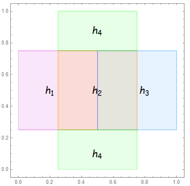
Lemma 7.4.

Let $G$ , $\mathbb{T}^{2}$ , and $\{W_{i}\}_{i=1}^{12}$ be defined as above. Fix $i\in V$ and let $x,y\in W_{i}$ . Then

d_{\mathbb{T}^{2}}(x,y)=d_{\mathbb{E}}(x,y).

Proof.

We only show that for any $x,y\in W_{1}$ ,

d_{\mathbb{T}^{2}}(x,y)=d_{\mathbb{E}}(x,y);

the proofs for $x,y\in W_{i}$ , $i=2,\ldots,8$ are the same. Let the four boundaries of $W_{1}$ be $l_{1},l_{2},l_{3},l_{4}$ , respectively (see Figure 2(b)). Let $x,y\in W_{1}$ , where $x$ is above $y$ , or at the same level. Then $d_{\mathbb{E}}(x,y)\leq\sqrt{2}/4.$ We prove that

d_{M}(x,y)<d_{\mathbb{E}}(x,y)

by considering the following eight cases:

Case 1. $x$ goes up to $l_{1}$ , goes through $W_{11},W_{8},W_{4}$ , and then back to the interior of $W_{1}$ .

Case 2. $x$ goes up to $l_{1}$ , then moves along $l_{1}$ by a distance $\geq 0$ , and finally back to the interior of $W_{1}$ .

Case 3. $x$ turns right and goes to $l_{4}$ , goes through $W_{2}$ all the way to the gluing edge, and goes from $l_{2}$ into the interior of $W_{1}$ .

Case 4. $x$ goes to the right to $l_{4}$ , then moves along $l_{4}$ by a distance $\geq 0$ , and finally returns to the interior of $W_{1}$ .

Case 5. $x$ turns left and goes to $l_{2}$ , then goes to the gluing edge, and finally traverses $W_{2}$ from $l_{4}$ into the interior of $W_{1}$ .

Case 6. $x$ turns left and goes to the $l_{2}$ , then moves along $l_{2}$ by a distance $\geq 0$ , and finally returns to the interior of $W_{1}$ .

Case 7. $x$ goes down to $l_{3}$ , then goes through $W_{4},W_{8},W_{11}$ , and finally goes back to the interior of $W_{1}$ .

Case 8. $x$ goes down to $l_{3}$ , then moves along $l_{3}$ by a distance $\geq 0$ , and finally returns to the interior of the $W_{1}$ .

For Case 1, it is easy to see that

d_{M}(x,y)\geq\frac{3}{4}>d_{\mathbb{E}}(x,y).

For Case 2, the triangular inequality implies that $d_{M}(x,y)>d_{\mathbb{E}}(x,y).$ Similarly, we can prove the other cases and thus complete the proof. ∎

Lemma 7.5.

Let $G=(V,E)$ , $\mathbb{T}^{2}$ , $\{W_{i}\}_{i=1}^{12}$ , and $\{S_{e}\}_{e\in E}$ be defined as above. Fix $i\in V$ and let $x,y\in W_{i}$ . Then

d_{\mathbb{T}^{2}}(S_{e}(x),S_{e}(y))=d_{\mathbb{E}}(S_{e}(x),S_{e}(x)).

Proof.

For the fixed $i\in V$ , by Remark 7.2, there exists some $j\in V$ such that $S_{e}(x),S_{e}(y)\subseteq W_{j}$ . By Lemma 7.4, we have

d_{\mathbb{T}^{2}}(S_{e}(x),S_{e}(y))=d_{\mathbb{E}}(S_{e}(x),S_{e}(x)).

∎

Example 7.6.

Let $G=(V,E)$ , $\mathbb{T}^{2}$ , $W$ , $\{h_{m}\}_{m=1}^{4}$ , $\{S_{e}\}_{e\in E}$ , and $K$ be defined as above. Let $\mu$ be an invariant measure of the GIFS $\{S_{e}\}_{e\in E}$ of bi-Lipschitz contractions on $W$ . Then $\underline{\operatorname{dim}}_{\infty}(\mu)>0$ . Consequently, the conclusions of Theorems 3.3, 4.3, and 5.3 hold for $\mu$ , and the conclusions of Theorems 3.4, 4.4, and 5.4 hold for all such $\mu$ and all $F\in{\rm Lip}(\operatorname{dom}\mathcal{E})$ .

Proof.

This follows by combining Lemmas 7.1 and 7.5. ∎

8. Example of solutions

In this section, we study weak solutions of linear wave, heat, and Schrödinger equations by using examples on $\mathbb{S}^{1}$ .

Example 8.1.

Let $M=\mathbb{S}^{1}:=\{(\cos(\theta+\pi/2),\sin(\theta+\pi/2)):\theta\in[-\pi,\pi]\}$ and let $\Omega:=\{(\cos(\theta+\pi/2),\sin(\theta+\pi/2)):\theta\in(-\pi/2,\pi/2)\}\subseteq M$ be an open set. Let $\mu$ be the Dirac point mass at the north pole $\theta=0$ . Then $\dim(L^{2}(\Omega,\mu))=1$ . Let

\displaystyle\varphi=\left\{\begin{aligned} &\frac{2\theta}{\pi}+1,\qquad\,\,\,\,&&\theta\in[-\pi/2,0],\\ &-\frac{2\theta}{\pi}+1,\qquad&&\theta\in(0,\pi/2].\\ \end{aligned}\right.

Then $\varphi$ is an eigenfunction of $-\Delta_{\mu}$ with $\lambda=4/\pi$ being an eigenvalue. Moreover, $\underline{\operatorname{dim}}_{\infty}(\mu)=0$ .

Proof.

We use the eigenvalues equation (see [32])

\displaystyle\int_{\Omega}(-\Delta\varphi)v\,d\nu=\lambda\int_{\Omega}\varphi v\,d\mu\qquad v\in C_{c}^{\infty}(\Omega).

Since

\int_{\Omega}(-\Delta\varphi)v\,d\nu=\int_{\Omega}\Big{(}\frac{4\delta_{0}}{\pi}\Big{)}v\,d\nu=\frac{4}{\pi}v\Big{(}\frac{\pi}{2}\Big{)}

and $\lambda\int_{\Omega}\varphi v\,d\mu=\lambda v(\pi/2)$ , we conclude that $4/\pi$ is an eigenvalue and $\varphi$ is an eigenfunction. ∎

Example 8.2.

Let $M$ , $\Omega$ , $\mu$ , $\varphi$ , and $\lambda$ be defined as in Example 8.1.

(a)

Let $g=\varphi/4$ , $h=0$ , and $f=0$ . Then the weak solution of the linear wave equation (3.4) is

$\displaystyle u(t)=\frac{\varphi}{4}\cos\Big{(}\frac{2t}{\sqrt{\pi}}\Big{)}.$

See Figure 3. Note that the solution is periodic.
(b)

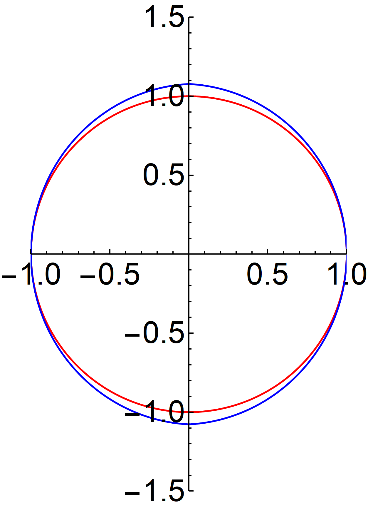
Let $g=\varphi/4$ and $f=c$ , where $c$ is constant. Then the weak solution of the linear heat equation (4.4) is

$\displaystyle u(t)=\frac{\varphi}{4}\big{(}e^{-4t/\pi}\big{(}1-c\pi\big{)}+c\pi\big{)}.$

See Figures 4–6. Note that if $c=0$ , then $u(t)$ tends to zero due to heat dissipation at the boundary points. If $c=1/8$ , $u(t)$ decreases as heat dissipation exceeds heat supply, and then it reaches an equilibrium when the rate of heat dissipation equals that rate of heat supply. If $c=3/4$ , $u(t)$ increases since heat supply exceeds heat dissipation, and again, $u(t)$ reaches an equilibrium when the rate of heat dissipation equals that of heat supply.
(c)

Let $g=\varphi/4$ and $f=0$ . Then the weak solution of the linear Schrödinger equation (5.4) is

$\displaystyle u(t)=\frac{\varphi}{4}e^{-i4t/\pi}.$

Note that both the real and imaginary parts of $u(t)$ exhibit periodic motion.

Example 8.3.

Let $M=\mathbb{S}^{1}:=\{(\cos(\theta+\pi/2),\sin(\theta+\pi/2)):-\pi\leq\theta\leq\pi\}$ . Let $\mu$ be two Dirac point mass at the north pole $\theta=0$ and the south pole $\theta=\pi$ . Let $\varphi_{1}=c_{1}$ and

\displaystyle\varphi_{2}=\left\{\begin{aligned} &\frac{2\theta}{\pi}+1&\qquad\theta\in[-\pi,0],\\ &\frac{-2\theta}{\pi}+1&\qquad\theta\in(0,\pi].\\ \end{aligned}\right.

Then $\varphi_{1}$ and $\varphi_{2}$ are eigenfunctions of $-\Delta_{\mu}$ with the corresponding eigenvalues are $\lambda_{1}=0$ and $\lambda_{2}=4/\pi$ , respectively. Moreover, $\underline{\operatorname{dim}}_{\infty}(\mu)=0$ .

The proof of Example 8.3 is similar to that of Example 8.1; we omit the proof.

Example 8.4.

Let $M$ , $\mu$ , $\varphi_{1}$ , $\varphi_{2}$ , and $\lambda$ be defined in Example 8.3.

(a)

Let $g=\varphi_{2}/4$ , $h=0$ , and $f=0$ . Then the weak solution of the linear wave equation (3.4) is

$\displaystyle u(t)=\frac{\varphi_{2}}{4}\cos\Big{(}\frac{2t}{\sqrt{\pi}}\Big{)}.$

Figure 7 shows the periodic wave motion.
(b)

Let $g=c_{1}+c_{2}\varphi_{2}$ and $f=c$ , where $c$ is a constant. Then the weak solution of the linear heat equation (4.4) is

$\displaystyle u(t)=c_{1}+\varphi_{2}\Big{(}e^{-4t/\pi}\Big{(}c_{2}-\frac{\pi}{4}c\Big{)}+\frac{\pi}{4}c\Big{)}.$

For example, if $c_{1}=1$ , $c_{2}=1$ , and $c=0$ , then $u(t)=1+\varphi_{2}e^{-4t/\pi}.$ In this case, the temperature of points in the upper semicircle decreases to 1, while that of points on the lower semicircle increases to 1. Total heat energy is conserved.
(c)

Let $g=\varphi_{2}/4$ and $f=0$ . Then the weak solution of the linear Schrödinger equation (5.4) is

$\displaystyle u(t)=\frac{\varphi_{2}}{4}e^{-i4t/\pi}.$

Figures 8 and 9 show the periodic behavior of $u(t)$ .

Acknowledgement

Part of this work was carried out while the second author was visiting Beijing Institute of Mathematical Sciences and Applications (BIMSA). She thanks the institute for its hospitality and support.

References

[1] R. A. Adams, Sobolev Spaces, Academic Press, New York, 1975.
[2] J. Ambjørn, J. Jurkiewicz and R. Loll, The spectral dimension of the universe is scale dependent, Phys. Rev. Lett. 95 (2005), 171301.
[3] D. Benedetti and J. Henson, Spectral geometry as a probe of quantum spacetime, Phys. Rev. D 80 (2009), 124036.
[4] E. J. Bird, S.-M. Ngai, and A. Teplyaev, Fractal Laplacians on the unit interval, Ann. Sci. Math. Qu $\acute{e}$ bec 27 (2003), 135–168.
[5] G. Calcagni, Fractal universe and quantum gravity, Phys. Rev. Lett. 104 (2010), 251301.
[6] G. Calcagni, Gravity on a multifractal, Phys. Lett. B 679 (2011), 251–253.
[7] K. Coletta, K. Dias, and R. S. Strichartz, Numerical analysis on the Sierpinski gasket, with applications to Schrödinger equations, wave equation, and Gibbs’ phenomenon, Fractals 12 (2004), 413–449.
[8] J. F.-C. Chan, S.-M. Ngai, and A. Teplyaev, One-dimensional wave equations defined by fractal Laplacians, J. Anal. Math. 127 (2015), 219–246.
[9] J. Chen and S.-M. Ngai, Eigenvalues and eigenfunctions of one-dimensional fractal Laplacians defined by iterated function systems with overlaps, J. Math. Anal. Appl. 364 (2010), 222–241.
[10] R. Cawley and R. D. Mauldin, Multifractal decompositions of Moran fractals, Adv. Math. 92 (1992), 196–236.
[11] E. B. Davies, Spectral Theory and Differential Operators, Cambridge Stud. Adv. Math., vol. 42, Cambridge Univ. Press, Cambridge, 1995.
[12] D.-W. Deng and S.-M. Ngai, Eigenvalue estimates for Laplacians on measure spaces, J. Funct. Anal. 268 (2015), 2231–2260.
[13] G. A. Edgar, Measure, Topology, and Fractal Geometry, Springer, New York, 1990.
[14] U. Freiberg, Analytical properties of measure geometric Kreĭn-Feller-operators on the real line, Math. Nachr. 260 (2003), 34–47.
[15] U. Freiberg, Spectral asymptotics of generalized measure geometric Laplacians on cantor like sets, Forum Math. 17 (2005), 87–104.
[16] U. Freiberg, Refinement of the spectral asymptotics of generalized Kreĭn Feller operators. Forum Math. 23 (2011), 427–445.
[17] U. Freiberg and M. Zähle, Harmonic calculus on fractals—a measure geometric approach, Potential Anal. 16 (2002), 265–277.
[18] Q. Gu, J. Hu, and S.-M. Ngai, Geometry of self-similar measures on intervals with overlaps and applications to sub-Gaussian heat kernel estimates, Commun. Pure Appl. Anal. 19 (2020), 641–676.
[19] R. M. Green, Spherical Astronomy, Cambridge Univ. Press, Cambridge, 1985.
[20] J. Hu, Nonlinear wave equations on a class of bounded fractal sets. J. Math. Anal. Appl. 270 (2002), 657–680.
[21] J. E. Hutchinson, Fractals and self-similarity, Indiana Univ. Math. J. 30 (1981), 713–747.
[22] J. Hu, K.-S. Lau, and S.-M. Ngai, Laplace operators related to self-similar measures on $\mathbb{R}^{d}$ , J. Funct. Anal. 239 (2006), 542–565.
[23] M. Kesseb $\ddot{o}$ hmer and A. Niemann, Spectral asymptotics of Kreĭn-Feller operators for weak Gibbs measures on self-conformal fractals with overlaps, Adv. Math. 403 (2022), Paper No. 108384.
[24] M. Kesseböhmer and A. Niemann, Spectral dimensions of Kreĭn-Feller operators and $L^{q}$ -spectra, Adv. Math. 399 (2022), Paper No. 108253.
[25] M. Kesseböhmer and A. Niemann, Spectral dimensions of Kreĭn-Feller operators in higher dimensions, arXiv: 2202.05247 (2022).
[26] J. Kigami, A harmonic calculus on the Sierpinski spaces, Japan J. Appl. Math. 6 (1989), 259–290.
[27] J. Kigami and M. L. Lapidus, Weyl’s problem for the spectral distribution of Laplacians on p.c.f. self-similar fractals, Comm. Math. Phys. 158 (1993), 93–125.
[28] R. D. Mauldin and S.C. Williams, Hausdorff dimension in graph directed constructions, Trans. Am. Math. Soc. 309 (1988), 811–829.
[29] K. Naimark and M. Solomyak, On the eigenvalue behaviour for a class of operators related to self-similar measures on $\mathbb{R}^{d}$ , C. R. Acad. Sci. Paris S $\acute{e}$ r. I Math. 319 (1994), 837–842.
[30] K. Naimark and M. Solomyak, The eigenvalue behaviour for the boundary value problems related to self-similar measures on $\mathbb{R}^{d}$ , Math. Res. Lett. 2 (1995), 279–298.
[31] S.-M. Ngai, Spectral asymptotics of Laplacians associated with one-dimensional iterated function systems with overlaps, Canad. J. Math. 63 (2011), 648–688.
[32] S.-M. Ngai and L. Ouyang, Kreĭn-Feller operators on Riemannian manifolds and a compact embedding theorem, arXiv:2301.06438 (2023).
[33] S.-M. Ngai and L. Ouyang, Hodge Theorem for Kreĭn-Feller operators on compact Riemannian manifolds, arXiv:2403.06182.
[34] S.-M. Ngai and W. Tang, Eigenvalue asymptotics and Bohr’s formula for fractal Schrödinger operators, Pacific J. Math. 300 (2019), 83–119.
[35] S.-M. Ngai and W. Tang, Schrödinger equations defined by a class of self-similar measures. J. Fractal Geom. 10 (2023), 209–241.
[36] S.-M. Ngai, W. Tang, and Y. Y. Xie, Spectral asymptotics of one-dimensional fractal Laplacians in the absence of second-order identities, Discrete Cont. Dyn. Syst. 38 (2018), 1849–1887.
[37] S.-M. Ngai, W. Tang, and Y. Y. Xie, Wave propagation speed on fractals, J. Fourier Anal. Appl. 26 (2020), 1–38.
[38] S.-M. Ngai and Y. Y. Xie, Spectral asymptotics of Laplacians related to one-dimensional graph-directed self-similar measures with overlaps, Ark. Mat. 58 (2020), 393–435.
[39] S.-M. Ngai and Y. Y. Xie, Spectral asymptotics of Laplacians associated with a class of higher-dimensional graph-directed self-similar measures, Nonlinearity 34 (2021), 5375–5398.
[40] S.-M. Ngai and Y. Y. Xu, Existence of $L^{q}$ -dimension and entropy dimension of self-conformal measures on Riemannian manifolds, Nonlinear Anal. 230 (2023), Paper No. 113226.
[41] S.-M. Ngai and Y. Y. Xu, Separation conditions for iterated function systems with overlaps on Riemannian manifolds, J. Geom. Anal. 33 (2023), no. 8, Paper No. 262.
[42] L. Olsen, Random Geometrically Graph Directed Self-Similar Multifractals, Pitman Res. Notes Math. Ser., vol. 307, New York, 1994.
[43] J. P. Pinasco and C. Scarola, Eigenvalue bounds and spectral asymptotics for fractal Laplacians, J. Fractal Geom. 6 (2019), 109–126.
[44] J. P. Pinasco and C. Scarola, A nodal inverse problem for measure geometric Laplacians, Commun Nonlinear Sci. Numer. Simul. 94 (2021), 105542.
[45] W. Tang and S.-M. Ngai, Heat equations defined by a class of self-similar measures with overlaps, Fractals 30 (2022), Paper No. 2250073.
[46] W. Tang and Z. Y. Wang, Strong damping wave equations defined by a class of self-similar measures with overlaps, J. Anal. Math. 150 (2023), 249–274.
[47] J. Wloka, Partial Differential Equations, Cambridge University Press, Cambridge, 1987.

		$\displaystyle\Big{\|}\int_{t}^{t+h}\sin(\sqrt{\lambda_{k}}(t+h-\tau))\gamma_{k}(\tau)d\tau\Big{\|}^{2}$
	$\displaystyle\leq$	$\displaystyle\int_{t}^{t+h}\big{\|}\sin(\sqrt{\lambda_{k}}(t+h))\cos(\sqrt{\lambda_{k}}\tau)-\cos(\sqrt{\lambda_{k}}(t+h))\sin(\sqrt{\lambda_{k}}(\tau))\big{\|}^{2}d\tau\int_{t}^{t+h}\big{\|}\gamma_{k}(\tau)\big{\|}^{2}d\tau$
	$\displaystyle=$	$\displaystyle\Big{(}\frac{h}{2}-\frac{\sin(2\sqrt{\lambda_{k}}h)}{4\sqrt{\lambda_{k}}}\Big{)}\int_{t}^{t+h}\big{\|}\gamma_{k}(\tau)\big{\|}^{2}d\tau$
	$\displaystyle\leq$	$\displaystyle\frac{h^{4}\lambda_{k}}{3}\mathop{\operatorname{ess\,sup}}\limits_{t\in[0,T]}\big{\|}\gamma_{k}(t)\big{\|}^{2},$

	$\displaystyle h_{1}\|_{W_{3}}=(S_{e_{7}}+S_{e_{8}}+S_{e_{9}})\|_{W_{3}},\qquad\qquad\qquad$	$\displaystyle h_{1}\|_{W_{4}}=(S_{e_{11}}+S_{e_{12}}+S_{e_{13}}+S_{e_{14}}+S_{e_{15}})\|_{W_{4}},$
	$\displaystyle h_{1}\|_{W_{7}}=(S_{e_{25}}+S_{e_{26}}+S_{e_{27}})\|_{W_{7}},\quad\qquad\qquad$	$\displaystyle h_{1}\|_{W_{8}}=(S_{e_{28}}+S_{e_{29}}+S_{e_{30}}+S_{e_{31}}+S_{e_{33}})\|_{W_{8}},$
	$\displaystyle h_{2}\|_{W_{4}}=(S_{e_{10}}+S_{e_{12}}+S_{e_{13}}+S_{e_{14}}+S_{e_{15}})\|_{W_{4}},$	$\displaystyle h_{2}\|_{W_{5}}=(S_{e_{17}}+S_{e_{18}}+S_{e_{19}}+S_{e_{20}}+S_{e_{21}})\|_{W_{5}},$
	$\displaystyle h_{2}\|_{W_{8}}=(S_{e_{28}}+S_{e_{29}}+S_{e_{30}}+S_{e_{31}}+S_{e_{32}})\|_{W_{8}},$	$\displaystyle h_{2}\|_{W_{9}}=(S_{e_{34}}+S_{e_{35}}+S_{e_{36}}+S_{e_{37}}+S_{e_{39}})\|_{W_{9}},$
	$\displaystyle h_{3}\|_{W_{5}}=(S_{e_{16}}+S_{e_{18}}+S_{e_{19}}+S_{e_{20}}+S_{e_{21}})\|_{W_{5}},$	$\displaystyle h_{3}\|_{W_{6}}=(S_{e_{22}}+S_{e_{23}}+S_{e_{24}})\|_{W_{6}},$
	$\displaystyle h_{3}\|_{W_{9}}=(S_{e_{34}}+S_{e_{35}}+S_{e_{36}}+S_{e_{37}}+S_{e_{38}})\|_{W_{9}},$	$\displaystyle h_{3}\|_{W_{10}}=(S_{e_{40}}+S_{e_{41}}+S_{e_{42}})\|_{W_{10}},$
	$\displaystyle h_{4}\|_{W_{1}}=(S_{e_{1}}+S_{e_{2}}+S_{e_{3}})\|_{W_{1}},\quad\qquad\qquad\qquad$	$\displaystyle h_{4}\|_{W_{2}}=(S_{e_{4}}+S_{e_{5}}+S_{e_{6}})\|_{W_{2}},$
	$\displaystyle h_{4}\|_{W_{11}}=(S_{e_{43}}+S_{e_{44}}+S_{e_{45}})\|_{W_{11}},\qquad\qquad$	$\displaystyle h_{4}\|_{W_{12}}=(S_{e_{46}}+S_{e_{47}}+S_{e_{48}})\|_{W_{12}}.$