Differentiable quantum chemistry with PySCF for molecules and materials at the mean-field level and beyond
Abstract
We introduce an extension to the PySCF package which makes it automatically differentiable. The implementation strategy is discussed, and example applications are presented to demonstrate the automatic differentiation framework for quantum chemistry methodology development. These include orbital optimization, properties, excited-state energies, and derivative couplings, at the mean-field level and beyond, in both molecules and solids. We also discuss some current limitations and directions for future work.
I Introduction
Automatic differentiation (AD) [1, 2] has recently become ubiquitous through its adoption in machine learning applications. AD removes the burden of implementing derivatives of complex computations by applying the chain rule to the elementary operations and functions of a computational graph. This can be used to automatically compute exact derivatives of arbitrary order.
In quantum chemistry, derivative evaluations appear in many types of calculations, such as in wavefunction optimization, to compute response properties, to obtain critical points and reaction paths on potential energy surfaces, in molecular dynamics simulations, for basis set and pseudopotential optimization, etc. Before the advent of AD, these derivatives were mainly computed by analytic schemes, where the symbolic formula for the derivative is first required (and which can be tedious to obtain), or computed numerically using finite difference methods (which are computationally expensive and prone to numerical instabilities). Both sets of difficulties are circumvented by applying AD, as shown in a few works very recently. For example, Tamayo-Mendoza et al.[3] implemented a fully differentiable Hartree–Fock (HF) method with AD; Song et al.[4] introduced an AD scheme to compute nuclear gradients for tensor hyper-contraction based methods; Abbott et al.[5] applied AD to calculations of higher order nuclear derivatives with methods such as HF, second-order Møller–Plesset perturbation theory (MP2) and coupled cluster theory with single, double and perturbative triple excitations [CCSD(T)]; and Kasim et al.[6] developed a differentiable quantum chemistry code called DQC for basis set optimizations, molecular property calculations etc. at the mean-field level. In addition, there are other quantum chemistry related applications where AD has played an important role, e.g., in training neural network based density functionals,[7, 8] in differentiable tensor network algorithms,[9] and in quantum circuit optimization.[10]
A central mission of PySCF [11, 12] is to provide a development platform to accelerate the implementation of new methods by its users. To further its potential, we have attempted to incorporate into PySCF the full functionality of AD. The resulting AD framework, which we call PySCFAD in the following, is available as an add-on to PySCF.[13] Although still in active development, we have found that PySCFAD is already very useful for derivative calculations associated with complex computational workflows. The purpose of this paper is thus to describe the current implementation of AD within PySCFAD and to illustrate its use in a range of applications.
The remainder of the paper is organized as follows. In section II, we discuss the implementation of a few key components in PySCFAD. In section III, example applications are presented to illustrate the capabilities of PySCFAD. In section IV, we examine the computational efficiency of PySCFAD. In section V, we summarize our experience with AD in this project, and outline some directions for future work.
II Implementation
We now describe the implementation of PySCFAD. We will assume some knowledge of the basics of AD; for further introduction see Ref. [2]. In PySCF, a majority of methods are implemented using NumPy[14] and SciPy[15] functions. These functions have differentiable counterparts provided by several advanced AD libraries.[16, 17, 18] (Here differentiable means that the function (or data) can be used or traced by an AD library in the computation of derivatives). Thus in many scenarios, transforming PySCF into PySCFAD is simply a matter of replacing the NumPy and SciPy functions with the corresponding differentiable ones from the AD library. However, there are also computationally heavy components such as the electron repulsion integrals (ERIs) which are implemented as C code in PySCF. We realize AD for these parts by registering the C functions that implement their analytic derivatives, which allows them to be called during the AD traversal of the computational graph. This not only avoids duplicate implementations of the same functionality, but also reduces the cost of AD tracing through complex numerical algorithms. Note, however, that such a strategy only allows for derivatives of finite order, as the C derivative functions appear as black-boxes to the AD framework.
Currently, we use Jax[18] as the backend AD package for PySCFAD. This is because besides being an AD library, Jax also provides other appealing features such as vectorization, parallelization, and just-in-time compilation, including for hardware accelerators. Using the strategy above, the following components of PySCF have been transformed to be compatible with automatic differentiation:
-
Molecular and crystal structures, Gaussian orbital evaluations and ERIs (gto and pbc/gto)
-
Molecular and plane wave density fitting routines (df and pbc/df)
-
HF and density functional theory (DFT) for molecules and solids (scf, dft, pbc/scf and pbc/dft)
-
Time-dependent HF and DFT (tdscf)
-
MP2 (mp)
-
Random phase approximation (gw)
-
Coupled cluster theory (cc)
-
Full configuration interaction (fci).
(The relevant modules in PySCF are listed in parentheses.) In the following, we give more details about the implementations of some of them.
II.1 Electron repulsion integrals
PySCF uses contracted Gaussian basis functions, the radial parts of which can be expressed as
| (1) |
where is the angular momentum, and the three parameters , and label the center, exponents and contraction coefficients, respectively. Differentiation of a basis function with respect to these variables leads to another Gaussian function. As such, derivatives of an ERI can be computed by a sequence of similar integral evaluations.
In the current implementation of PySCFAD, the program walks through the computation graph and determines the required intermediate ERIs. For example, computing the second order derivative of the one-electron overlap integral with respect to the basis function centers requires the evaluation of three integrals
where in the above, the permutation symmetries have been considered. In the implementation, these integrals are all evaluated analytically by the highly optimized integral library Libcint.[19] Thus, the ERIs themselves are treated as elementary functions during the AD procedure, instead of the lower-level arithmetic operations that compute them.
For the commonly used ERIs, up to fourth order derivatives with respect to the basis function centers are available through Libcint. If higher order derivatives are needed, one can extend Libcint by generating the code to compute the required intermediate integrals before runtime, with the accompanying automatic code generator. Only first order derivatives with respect to the exponents and contraction coefficients have been implemented so far. This should be sufficient for many purposes, such as for basis function optimization.
The procedure above, in a strict sense, is not fully differentiable, because the ERI evaluation is black-box. However, a general, efficient and fully differentiable implementation for the ERIs remains challenging. The advent of compiler level AD tools[20] may facilitate such developments in the future.
II.2 Density functionals
A semi-local exchange correlation (XC) density functional can be expressed as
| (2) |
where is the XC energy per particle, and and label the electron density and the non-interacting kinetic energy density, respectively. The integration in Eq. 2 is usually carried out numerically over a quadrature grid due to the complexity of XC functionals:
| (3) |
where is the weight for the -th grid point at position . The AD of is straightforward if one uses a fully differentiable implementation of . However, we do not pursue that strategy here, since density derivatives to finite order (usually up to fourth order) are sufficient in most practical scenarios and these have already been implemented in efficient density functional libraries such as Libxc.[21] Therefore, we take an approach similar to that introduced above for the AD of ERIs, where the derivatives of with respect to the density variables are computed analytically, while other derivatives (e.g., the derivatives of the density variables) are generated by AD. In particular, Libxc provides analytic functional derivatives of , from which the derivatives of can be easily expressed. For example, the first order derivative of with respect to within the local density approximation (LDA) is obtained as
| (4) |
where both and (the XC potential) are computed analytically by Libxc. The higher order derivatives are obtained by recursion, e.g.,
| (5) |
where is the XC kernel.
II.3 Eigendecompositions
Although Jax provides a differentiable implementation of the eigendecomposition, it does not handle degenerate eigenstates. Usually, in order to determine the derivatives of degenerate eigenstates, one needs to diagonalize the perturbations of the matrix being decomposed within the degenerate subspace until the degeneracy is removed. Such an approach, however, is not well defined for reverse-mode AD, because the basis in which to expand the degenerate eigenstates is undetermined until the back propagation is carried out. The development of a general differentiable eigensolver is beyond the scope of the current work. In the following, we only discuss a workaround for the AD of eigenvalue problems arising in mean-field calculations.
At the mean-field level, a gauge invariant quantity will only respond to perturbations that mix occupied and unoccupied states. Thus in many cases, the response of degenerate single-particle eigenstates, i.e. orbitals (which can only be either occupied or unoccupied for gapped systems) does not contribute to the derivatives, and can be ignored. Our implementation directly follows the standard analytic formalism derived from linear response theory.[22] For a generalized eigenvalue problem
| (6) |
where and denote the eigenvalue and eigenvector matrices, respectively, their differentials can be expressed as
| (7) |
and
| (8) |
respectively. In the two equations above, represents element-wise multiplication,
| (9) |
and
| (10) |
Similar approaches have also been reported in other works.[9, 8]
II.4 Implicit differentiation of iterative solvers
Automatic differentiation of optimization problems or iterative solvers is usually done in one of two ways, namely, unrolling the iterations[1, 23] or implicit differentiation.[2, 24, 25]
In the first approach, the entire set of iterations is differentiated, leading to a memory complexity that scales linearly with the number of iterations for reverse-mode AD. In addition, the so-obtained derivatives are usually initial guess dependent. This can be understood with the example of computing the molecular orbital (MO) response (Eq. 8). Suppose in an extreme case that the self-consistent field (SCF) iteration takes the converged MOs as the initial guess, then the SCF will converge after one Fock matrix diagonalization. Due to the fact the SCF iteration is short-circuited (the Fock matrix is not rebuilt) the input MOs have no knowledge of their own derivatives, and the Fock matrix, which responds to the MO changes, will have the wrong derivative after this single SCF iteration, which in turn leads to the wrong MO response. In other words, self-consistency is not reached when solving Eq. 8, where depends on ; the quality of convergence of the self-consistent response equations is controlled only by the threshold of the SCF itself. Such errors can be corrected by increasing the number of SCF iterations, so that the Fock matrix response with respect to the MO changes is gradually restored, and self-consistency of Eq. 8 is achieved. To see this effect, we computed the nuclear gradient of N2 molecule at the MP2 level, where the derivatives of the MO coefficients are evaluated by the scheme of unrolling the SCF iterations. Using the same set of converged MOs as the initial guess, we vary the number of SCF iterations and plot the gradient error, shown as the red curve in Fig. 1. It is clear that the computed gradient is inaccurate unless a sufficient number of SCF iterations are carried out to recover the correct MO response. Nevertheless, the method is problematic when performing AD for optimizations or for iterative solvers, as one has no direct control over the convergence of the computed derivatives.
In implicit differentiation, instead of differentiating the solver iterations, the optimality condition is implicitly differentiated. For example, the solution (denoted as ) of the iterative solver should also be the root of some optimality condition
| (11) |
According to the implicit function theorem,[26, 2] can be seen as an implicit function of , and its derivative can be obtained by solving a set of linear equations
| (12) |
In the problem of computing the MO response, Eq. 12 simply corresponds to the coupled perturbed Hartree-Fock (CPHF) equations.[22] More interestingly, in the reverse-mode AD, one does not directly solve Eq. 12; instead, the vector Jacobian product (i.e., where is a vector and ) is computed. If we define and , then the vector Jacobian product is obtained as
| (13) |
where
| (14) |
In this case, only one set of linear equations (Eq. 14) needs to be solved even if derivatives are evaluated with respect to multiple variables (i.e., when changes but not and ). Note that Eqs. 13 and 14 correspond exactly to the -vector approach[27] in conventional analytic derivative methods.
The advantages of the implicit differentiation approach are obvious. First, because only the optimality condition is differentiated, the computational complexity and memory footprint do not depend on the actual implementation of the solver or on the number of solver iterations. A notable benefit of this is that algorithms to accelerate convergence can be readily applied, such as the direct inversion of the iterative subspace[28] (DIIS) method, without any modification to the AD implementation. (Note, however, that Eq. 14 itself needs to be solved iteratively, which can be more expensive than the approach of unrolling the iterations, depending on the size and convergence of the problem). Second, the computed derivatives have errors that are governed only by the accuracy of the solution of Eq. 14, which can be controlled with a predefined convergence threshold. This can be seen from the blue curve in Fig. 1, where the implicit differentiation approach is applied for the same MP2 nuclear gradient calculation as discussed above.
Given a general implementation,[25] implicit differentiation can be applied to almost any iterative solver. Currently, we have adapted it for the AD of SCF iterations and the coupled cluster (CC) amplitude equations. This eliminates the need to explicitly implement and solve the CPHF equations and the CC equations.[29] Finally, it is interesting to mention that if the optimality condition being differentiated involves the fixed point problem of gauge variant quantities (e.g., wavefunctions), it is important to fix the gauge. In particular, the fixed point of the optimality condition should be identical to the variable used to evaluate the objective function.

III Applications
In this section, we provide a few examples that demonstrate the capabilities of PySCFAD. In addition, complete code snippets are presented to highlight the ease of developing new methodologies within the framework of PySCFAD. Reverse-mode AD was applied in all the following calculations, although PySCFAD also allows forward-mode AD for its functions.
III.1 Orbital optimization
Orbital optimization in electronic structure methods provides the following advantages:
-
1.
Energies become variational with respect to orbital rotations, thus there is no need for orbital response when computing nuclear gradients.[30]
-
2.
Properties can be computed more easily because there are no orbital response contributions to the density matrices.
-
3.
The spurious poles in response functions for inexact methods such as coupled cluster theory can be removed.[31]
-
4.
Symmetry breaking problems may be described better.[32]
However, it is not always straightforward to implement analytic orbital gradients (and hessians for quadratically convergent optimization) if the underlying electronic structure method is complicated. In contrast, little effort is needed to obtain the orbital gradients and hessians using AD as long as the energy can be defined and implemented as differentiable with respect to orbital rotations.
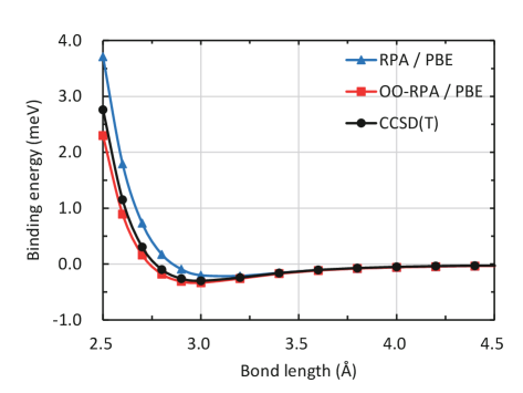
As an example, in Fig. 2, we show the application of orbital optimization to the random phase approximation for the energy[33, 34, 35] (RPA) within the framework of PySCFAD. The base RPA method is implemented following Ren et al.,[36] where the correlation energy is evaluated by numerical integration over the imaginary frequency axis and density fitting is applied to reduce the computation cost. The total energy is then minimized with respect to the orbital rotation , where is anti-hermitian and its upper triangular part corresponds to the variable “x” in Fig. 2. Note that only the energy function needs to be explicitly implemented (lines 24–31 in Fig. 2), whereas the orbital gradient and hessian (specifically, the hessian-vector product in the example) are obtained directly by AD (lines 33–36 in Fig. 2). The performance of the resulting orbital optimized (OO) RPA method is shown in Fig. 3. We plot the binding energy curves for the He2 molecule computed at the RPA, OO-RPA and CCSD(T) levels. It is clear that the molecule is underbound at the RPA level, whereas applying orbital optimization corrects that and the binding energies are more consistent with the CCSD(T) results.

III.2 Response properties
In general, ground-state dynamic (frequency-dependent) response properties are related to the derivatives of the quasienergy with respect to perturbations.[37] The quasienergy is defined as the time-averaged expectation value of over the phase-isolated time-dependent wavefunction.[37] As such, although there is no difficulty applying AD to compute such derivatives, a straightforward application to the quasienergy in this form requires the time-dependent wavefunction itself. In the time-independent limit, however, the quasienergy reduces to the usual energy, thus the static response properties can be computed straightforwardly with AD from only time-independent quantities.
For example, the static Raman activity is related to the susceptibility[38, 39]
| (15) |
where is the ground-state energy, denotes the nuclear coordinates, and represents the electric-field. In Fig. 4, we present an implementation of Raman activity at the CCSD level within the framework of PySCFAD. Again, only the energy function needs to be explicitly implemented (lines 14–24 in Fig. 4), while all the derivatives are obtained by AD (lines 27 and 32 in Fig. 4). In particular, the CPHF and CC equations are solved implicitly through the implicit differentiation procedure. Using this code, we compute the harmonic vibrational frequency, Raman activity and depolarization ratio for the BH molecule, and the results are displayed in Table 1. It can be seen that they agree very well with the reference analytic results, which validates our AD implementation.
Similarly, the IR intensity, which involves computing the nuclear derivative of the dipole moment, can be obtained in the same manner with AD. In Table 2, the IR intensities of the H2O molecule at the CCSD level are displayed. Both AD and analytic evaluation give almost identical results.

| Properties | PySCFAD | Referencea |
|---|---|---|
| Frequency (cm-1) | 2336.70 | 2337.24 |
| Raman activity (Åamu) | 217.84 | 215.11 |
| Depolarization ratio | 0.56 | 0.56 |
-
a Reference values obtained from Ref. 39.
| Modes | Frequency (cm-1) | IR intensity (km/mol) | |||
|---|---|---|---|---|---|
| PySCFAD | Referencea | PySCFAD | Referencea | ||
| 1 | 3844 | 3846 | 4.47 | 4.45 | |
| 2 | 1700 | 1697 | 56.41 | 56.15 | |
| 3 | 3956 | 3950 | 22.64 | 22.62 | |
-
a Reference values obtained from the computational chemistry comparison and benchmark database.[40]
III.3 Excitation energies
Excitation energies can be identified from the poles of response functions, and can be obtained by solving the (generalized) eigenvalue problems which arise from the derivatives of quasienergy Lagrangians.[37] For example, in coupled cluster theory, the excitation energies can be computed as the eigenvalues of the CC Jacobian, which is defined as the second order derivative of the zeroth order Lagrangian with respect to the amplitudes and to the multipliers:
| (16) |
Note that gives the CC amplitude equations, which are already implemented in the ground state CC methods. Therefore, the CC Jacobian and subsequently the excitation energies can be obtained effortlessly if AD is applied to differentiate the amplitude equations. In Fig. 5, we show such an example of computing the excitation energies at the CCSD level, where only the CC amplitude equations are explicitly implemented (line 29 in Fig. 5), while the CC Jacobian is obtained via AD (line 33 Fig. 5) and is then diagonalized. The resulting excitation energies are identical to those from the equation-of-motion (EOM) method (see Table 3). Note that it is also possible to only compute the Jacobian vector product rather than the full Jacobian (similar to line 36 in Fig. 2), so that the diagonalization can be performed with Krylov subspace methods,[41] making larger calculations practical.
The strategy above is in principle applicable to any method, with the caveat that complications may arise depending on the particular ansatz used for representing the wavefunction. In general, the eigenvalue problem being solved has the form
| (17) |
where is the second order derivative of the zeroth order energy or Lagrangian, and may be related to the second order derivative of the wavefunction overlap, which may or may not be the identity.

| States | PySCFADa | Referenceb |
|---|---|---|
| S1 | 0.463 | 0.463 |
| S2 | 0.735 | 0.735 |
| S3 | 1.096 | 1.096 |
| S4 | 1.152 | 1.152 |
-
a Excitation energies computed by diagonalizing the CC Jacobian from AD.
-
b Reference values computed by the EOM-EE-CCSD method.
III.4 Derivative coupling
The first order derivative coupling between two electronic states and is defined as[42, 43]
| (18) |
where denotes the nuclear coordinates. Although derivative couplings are closely related to excited-state nuclear gradients, their analytic derivation and implementation may still be tedious and error-prone, depending on the complexity of the underlying electronic structure methods. However, such calculations can be greatly simplified by applying AD.
In Fig. 6, we give an example of computing the derivative coupling at the full configuration interaction[44] (FCI) level within PySCFAD. It should be noted that only a very simple function is explicitly implemented and then differentiated by AD, which is the wavefunction overlap . The here emphasizes that does not respond to the perturbation. In practice, all the variables corresponding to are held constant when defining the objective function (e.g., “mol”, “fcivec” and “mf.mo_coeff” at lines 24–26 in Fig. 6).
The strategy above is applicable to any wavefunction method. In Table 4, we compare the derivative couplings computed at the configuration interaction singles[45] (CIS) and FCI levels. It is clear that the two methods give very different results. Nevertheless, our AD implementation produces exactly the same results as the reference implementation. In addition, second order derivative couplings can be readily obtained by performing AD on the same wavefunction overlap another time. Finally, with AD, it is even more straightforward to compute the Hellmann-Feynman part of the derivative coupling (which is translationally invariant,[46, 47] unlike the full derivative coupling)
| (19) |
where is the Hamiltonian represented in a certain Hilbert space and denotes the eigenvectors (i.e., CI vectors) of . Here, only the Hamiltonian needs to be differentiated (with the orbital response taken into account), but the CI vectors are treated as constants. In other words, it is not necessary to differentiate the CI eigensolver (e.g., the Davidson iterations[48]), which greatly simplifies the problem.

| Methods | PySCFAD | Reference |
|---|---|---|
| CIS | 0.0796 | 0.0796a |
| FCI | 0.2126 | 0.2126b |
-
a Reference values computed analytically by Q-Chem.[49]
-
b Reference values computed by finite difference.
III.5 Property calculation for solids
The PySCFAD framework also works seamlessly for solid calculations. Here, we give an example of computing the stress tensor to illustrate this.
The stress tensor is defined as the first order energy response to the infinitesimal strain deformation[50]
| (20) |
where and are the energy and volume of a unit cell, respectively, and the strain tensor defines the transformation of real space coordinates according to
| (21) |
in which and denote the Cartesian components. The strain deformation applies to both nuclear coordinates and lattice vectors, which also implicitly affects the derived quantities such as the reciprocal lattice vectors and the unit cell volume.
In Fig. 7, the stress tensor for a two-atom Si primitive cell is computed by AD at the Hartree-Fock level, where a mixed Gaussian and plane wave approach (plane-wave density fitting) is used.[51, 52] The results are plotted in Fig. 8 along with the corresponding finite difference values. Perfect agreement is obtained with an average discrepancy of eV/Å3 between the AD and finite difference results. It should be noted that in this case, the plane wave basis (i.e., the uniform grid point) response to the strain deformation is non-negligible, which subsequently requires differentiation with respect to the grid points. However, all these complications are hidden from the user, and it suffices to modify the energy function (as shown in Fig. 7) for the gradient calculations.


IV Computational efficiency
In this section, we investigate the computation cost for carrying out typical quantum chemistry calculations within the PySCFAD framework.
First, we consider objective function evaluation. As an example, in Fig. 9, we plot the computation time for computing the CCSD(T) energy of the H2O molecule using the implementations in PySCF and PySCFAD, respectively. The main difference between the two implementations is that PySCF respects the 8-fold permutation symmetry of the two-electron repulsion integrals, while no such symmetry is enforced in PySCFAD. For PySCFAD, we also compare the performance of applying Jax and NumPy as the tensor operation backends, respectively. The corresponding results are presented as the red (PySCF), blue and orange (PySCFAD with Jax), and gray (PySCFAD with NumPy) bars in Fig. 9. We see that PySCFAD with the Jax backend is about times less efficient than PySCF, which is due to the lack of integral symmetries. However, PySCFAD with the NumPy backend performs much worse for larger calculations. This is mainly because the einsum function in NumPy, when applied to general tensor contractions, may be less optimized and only runs on a single core. With the Jax backend, the same function is optimized by XLA[54] (accelerated linear algebra), which greatly improves the computation efficiency, although the just-in-time compilation introduces some overhead, as shown by the orange bars in Fig. 9. Overall, this suggest that it is potentially possible for PySCFAD to be just as efficient as PySCF for objective function evaluation, if the implementation is carefully optimized.
Second, we examine the efficiency of AD for derivative calculations. In Fig. 10, the computation time for CCSD nuclear gradients of H2O molecule using the analytic implementation in PySCF and the AD procedures in PySCFAD is plotted. Note that two iterative solvers are involved in the CCSD energy evaluation, i.e., the SCF iteration and the CC amplitude equation. When applying AD to compute the gradient, one can choose to use either the approach of unrolling the iterations or the implicit differentiation of the two iterative solvers. As such, the performance of these AD approaches are also compared, as displayed by the three sets of blue bars in Fig. 10. It is clear that all the AD calculations are less efficient than the analytic evaluations by a factor of , which is again due to the lack of integral symmetries. On the other hand, the different AD approaches give comparable performance in terms of the computation time. However, implicit differentiation of the iterative solvers consumes a considerably smaller amount of memory than unrolling the iterations. In more detail, for the case of the cc-pVQZ basis set in Fig. 10, more than 20 gigabytes of memory are used to store the intermediate quantities for computing the gradients of the ERIs, which applies equally to all the AD approaches. The remaining memory can be associated with the iterative solvers, and we find that implicit differentiation of the SCF and CC iterations reduces the associated memory usage by a factor of compared to the approach of unrolling the iterations. In conclusion, PySCFAD appears to be computationally efficient for derivative evaluations, especially when the iterative solvers are differentiated implicitly.


V Conclusions
In this work, we introduced PySCFAD, a differentiable quantum chemistry framework based on PySCF. It facilitates derivative calculations for complex computational workflows, and can be applied to both molecular and periodic systems, at the mean-field level and beyond. Using PySCFAD, new quantum chemistry methods can be implemented in a differentiable way with almost no extra effort. As such, we expect it to become a useful platform to rapidly prototype new methodologies, which can then be benchmarked on properties that were previously difficult to compute due to the lack of analytic derivatives. At the current point, there remain a few challenges to be addressed in the future developments of PySCFAD.
-
1.
Jax is less efficient than NumPy unless the Python functions are compiled with XLA. However, this is not always possible, especially when Python control flows are involved. As such, code optimization becomes more difficult for PySCFAD.
-
2.
Incorporating permutation symmetries in electron integrals is tricky, because it requires element-wise in-place array updates, which are extremely inefficient with current AD tools.
-
3.
The current implementation amounts to an “in-core” version of all methods, i.e., all the data is stored in memory. For “out-core” implementations where data can be stored on disk, additional work is needed to the track the history of the data, without which gradient propagation cannot proceed.
Acknowledgements.
This work was supported by the US Department of Energy through the US DOE, Office of Science, Basic Energy Sciences, Chemical Sciences, Geosciences, and Biosciences Division under Triad National Security, LLC (“Triad”) contract Grant 89233218CNA000001. Support for PySCF ML infrastructure on top of which PySCFAD was built comes from the Dreyfus Foundation.Data availability statement
The data that support the findings of this study are available from the corresponding author upon reasonable request. The PySCFAD source code can be found at https://github.com/fishjojo/pyscfad.
References
- Wengert [1964] R. E. Wengert, “A simple automatic derivative evaluation program,” Communications of the ACM 7, 463–464 (1964).
- Griewank and Walther [2008] A. Griewank and A. Walther, Evaluating Derivatives (Society for Industrial and Applied Mathematics, 2008).
- Tamayo-Mendoza et al. [2018] T. Tamayo-Mendoza, C. Kreisbeck, R. Lindh, and A. Aspuru-Guzik, “Automatic differentiation in quantum chemistry with applications to fully variational hartree–fock,” ACS Central Science 4, 559–566 (2018).
- Song, Martínez, and Neaton [2020] C. Song, T. J. Martínez, and J. B. Neaton, “An automatic differentiation and diagrammatic notation approach for developing analytical gradients of tensor hyper-contracted electronic structure methods,” chemrxiv (2020), 10.26434/chemrxiv.13002965.v1.
- Abbott et al. [2021] A. S. Abbott, B. Z. Abbott, J. M. Turney, and H. F. Schaefer, “Arbitrary-order derivatives of quantum chemical methods via automatic differentiation,” Journal of Physical Chemistry Letters 12, 3232–3239 (2021).
- Kasim, Lehtola, and Vinko [2022] M. F. Kasim, S. Lehtola, and S. M. Vinko, “Dqc: A python program package for differentiable quantum chemistry,” Journal of Chemical Physics 156 (2022), 10.1063/5.0076202.
- Li et al. [2021] L. Li, S. Hoyer, R. Pederson, R. Sun, E. D. Cubuk, P. Riley, and K. Burke, “Kohn-sham equations as regularizer: Building prior knowledge into machine-learned physics,” Physical Review Letters 126 (2021), 10.1103/PhysRevLett.126.036401.
- Kasim and Vinko [2021] M. F. Kasim and S. M. Vinko, “Learning the exchange-correlation functional from nature with fully differentiable density functional theory,” (2021), 10.1103/PhysRevLett.127.126403.
- Liao et al. [2019] H. J. Liao, J. G. Liu, L. Wang, and T. Xiang, “Differentiable programming tensor networks,” Physical Review X 9 (2019), 10.1103/PhysRevX.9.031041.
- Arrazola et al. [2021] J. M. Arrazola, S. Jahangiri, A. Delgado, J. Ceroni, J. Izaac, A. Száva, U. Azad, R. A. Lang, Z. Niu, O. D. Matteo, R. Moyard, J. Soni, M. Schuld, R. A. Vargas-Hernández, T. Tamayo-Mendoza, C. Y.-Y. Lin, A. Aspuru-Guzik, and N. Killoran, “Differentiable quantum computational chemistry with pennylane,” (2021).
- Sun et al. [2018] Q. Sun, T. C. Berkelbach, N. S. Blunt, G. H. Booth, S. Guo, Z. Li, J. Liu, J. D. McClain, E. R. Sayfutyarova, S. Sharma, S. Wouters, and G. K. L. Chan, “Pyscf: the python-based simulations of chemistry framework,” Wiley Interdisciplinary Reviews: Computational Molecular Science 8, e1340 (2018).
- Sun et al. [2020] Q. Sun, X. Zhang, S. Banerjee, P. Bao, M. Barbry, N. S. Blunt, N. A. Bogdanov, G. H. Booth, J. Chen, Z.-H. Cui, J. J. Eriksen, Y. Gao, S. Guo, J. Hermann, M. R. Hermes, K. Koh, P. Koval, S. Lehtola, Z. Li, J. Liu, N. Mardirossian, J. D. McClain, M. Motta, B. Mussard, H. Q. Pham, A. Pulkin, W. Purwanto, P. J. Robinson, E. Ronca, E. R. Sayfutyarova, M. Scheurer, H. F. Schurkus, J. E. T. Smith, C. Sun, S.-N. Sun, S. Upadhyay, L. K. Wagner, X. Wang, A. White, J. D. Whitfield, M. J. Williamson, S. Wouters, J. Yang, J. M. Yu, T. Zhu, T. C. Berkelbach, S. Sharma, A. Y. Sokolov, and G. K.-L. Chan, “Recent developments in the p ¡scp¿y¡/scp¿ scf program package,” The Journal of Chemical Physics 153, 024109 (2020).
- Zhang, Yang, and Chan [2022] X. Zhang, J. Yang, and G. K.-L. Chan, “Pyscf with auto-differentiation,” (2022).
- Harris et al. [2020] C. R. Harris, K. J. Millman, S. J. van der Walt, R. Gommers, P. Virtanen, D. Cournapeau, E. Wieser, J. Taylor, S. Berg, N. J. Smith, R. Kern, M. Picus, S. Hoyer, M. H. van Kerkwijk, M. Brett, A. Haldane, J. F. del Río, M. Wiebe, P. Peterson, P. Gérard-Marchant, K. Sheppard, T. Reddy, W. Weckesser, H. Abbasi, C. Gohlke, and T. E. Oliphant, “Array programming with numpy,” (2020).
- Virtanen et al. [2020] P. Virtanen, R. Gommers, T. E. Oliphant, M. Haberland, T. Reddy, D. Cournapeau, E. Burovski, P. Peterson, W. Weckesser, J. Bright, S. J. van der Walt, M. Brett, J. Wilson, K. J. Millman, N. Mayorov, A. R. Nelson, E. Jones, R. Kern, E. Larson, C. J. Carey, İlhan Polat, Y. Feng, E. W. Moore, J. VanderPlas, D. Laxalde, J. Perktold, R. Cimrman, I. Henriksen, E. A. Quintero, C. R. Harris, A. M. Archibald, A. H. Ribeiro, F. Pedregosa, P. van Mulbregt, A. Vijaykumar, A. P. Bardelli, A. Rothberg, A. Hilboll, A. Kloeckner, A. Scopatz, A. Lee, A. Rokem, C. N. Woods, C. Fulton, C. Masson, C. Häggström, C. Fitzgerald, D. A. Nicholson, D. R. Hagen, D. V. Pasechnik, E. Olivetti, E. Martin, E. Wieser, F. Silva, F. Lenders, F. Wilhelm, G. Young, G. A. Price, G. L. Ingold, G. E. Allen, G. R. Lee, H. Audren, I. Probst, J. P. Dietrich, J. Silterra, J. T. Webber, J. Slavič, J. Nothman, J. Buchner, J. Kulick, J. L. Schönberger, J. V. de Miranda Cardoso, J. Reimer, J. Harrington, J. L. C. Rodríguez, J. Nunez-Iglesias, J. Kuczynski, K. Tritz, M. Thoma, M. Newville, M. Kümmerer, M. Bolingbroke, M. Tartre, M. Pak, N. J. Smith, N. Nowaczyk, N. Shebanov, O. Pavlyk, P. A. Brodtkorb, P. Lee, R. T. McGibbon, R. Feldbauer, S. Lewis, S. Tygier, S. Sievert, S. Vigna, S. Peterson, S. More, T. Pudlik, T. Oshima, T. J. Pingel, T. P. Robitaille, T. Spura, T. R. Jones, T. Cera, T. Leslie, T. Zito, T. Krauss, U. Upadhyay, Y. O. Halchenko, and Y. Vázquez-Baeza, “Scipy 1.0: fundamental algorithms for scientific computing in python,” Nature Methods 17, 261–272 (2020).
- Walter and Lehmann [2013] S. F. Walter and L. Lehmann, “Algorithmic differentiation in python with algopy,” Journal of Computational Science 4, 334–344 (2013).
- Paszke et al. [2017] A. Paszke, S. Gross, S. Chintala, G. Chanan, E. Yang, Z. D. Facebook, A. I. Research, Z. Lin, A. Desmaison, L. Antiga, O. Srl, and A. Lerer, “Automatic differentiation in pytorch,” (2017).
- Bradbury et al. [2018] J. Bradbury, R. Frostig, P. Hawkins, M. J. Johnson, C. Leary, D. Maclaurin, G. Necula, A. Paszke, J. VanderPlas, S. Wanderman-Milne, and Q. Zhang, “JAX: composable transformations of Python+NumPy programs,” (2018).
- Sun [2015] Q. Sun, “Libcint: An efficient general integral library for gaussian basis functions,” Journal of Computational Chemistry 36, 1664–1671 (2015).
- Moses and Churavy [2020] W. Moses and V. Churavy, “Instead of rewriting foreign code for machine learning, automatically synthesize fast gradients,” in Advances in Neural Information Processing Systems, Vol. 33, edited by H. Larochelle, M. Ranzato, R. Hadsell, M. F. Balcan, and H. Lin (Curran Associates, Inc., 2020) pp. 12472–12485.
- Lehtola et al. [2018] S. Lehtola, C. Steigemann, M. J. Oliveira, and M. A. Marques, “Recent developments in libxc — a comprehensive library of functionals for density functional theory,” SoftwareX 7, 1–5 (2018).
- Pople et al. [1979] J. A. Pople, R. Krishnan, H. B. Schlegel, and J. S. Binkley, “Derivative studies in hartree-fock and møller-plesset theories,” International Journal of Quantum Chemistry 16, 225–241 (1979).
- Ablin, Peyré, and Moreau [2020] P. Ablin, G. Peyré, and T. Moreau, “Super-efficiency of automatic differentiation for functions defined as a minimum,” in International Conference on Machine Learning (PMLR, 2020) pp. 32–41.
- Andersson et al. [2019] J. A. Andersson, J. Gillis, G. Horn, J. B. Rawlings, and M. Diehl, “Casadi: a software framework for nonlinear optimization and optimal control,” Mathematical Programming Computation 11, 1–36 (2019).
- Blondel et al. [2021] M. Blondel, Q. Berthet, M. Cuturi, R. Frostig, S. Hoyer, F. Llinares-López, F. Pedregosa, and J.-P. Vert, “Efficient and modular implicit differentiation,” (2021).
- Krantz and Parks [2002] S. G. Krantz and H. R. Parks, The implicit function theorem: history, theory, and applications (Springer Science & Business Media, 2002).
- Handy and Schaefer [1984] N. C. Handy and H. F. Schaefer, “On the evaluation of analytic energy derivatives for correlated wave functions,” The Journal of Chemical Physics 81, 5031–5033 (1984).
- Pulay [1982] P. Pulay, “Improved scf convergence acceleration,” Journal of Computational Chemistry 3, 556–560 (1982).
- Scheiner et al. [1987] A. C. Scheiner, G. E. Scuseria, J. E. Rice, T. J. Lee, and H. F. Schaefer, “Analytic evaluation of energy gradients for the single and double excitation coupled cluster (ccsd) wave function: Theory and application,” The Journal of Chemical Physics 87, 5361–5373 (1987).
- Rendell et al. [1987] A. P. Rendell, G. B. Bacskay, N. S. Hush, and N. C. Handy, “The analytic configuration interaction gradient method: The calculation of one electron properties,” The Journal of Chemical Physics 87, 5976–5986 (1987).
- Pedersen, Fernández, and Koch [2001] T. B. Pedersen, B. Fernández, and H. Koch, “Gauge invariant coupled cluster response theory using optimized nonorthogonal orbitals,” Journal of Chemical Physics 114, 6983–6993 (2001).
- Sherrill et al. [1998] C. D. Sherrill, A. I. Krylov, E. F. Byrd, and M. Head-Gordon, “Energies and analytic gradients for a coupled-cluster doubles model using variational brueckner orbitals: Application to symmetry breaking in o4+,” (1998).
- Bohm and Pines [1953] D. Bohm and D. Pines, “A collective description of electron interactions: Iii. coulomb interactions in a degenerate electron gas,” Physical Review 92, 609–625 (1953).
- Gell-Mann and Brueckner [1957] M. Gell-Mann and K. A. Brueckner, “Correlation energy of an electron gas at high density,” Physical Review 106, 364–368 (1957).
- Furche [2001] F. Furche, “Molecular tests of the random phase approximation to the exchange-correlation energy functional,” Physical Review B - Condensed Matter and Materials Physics 64 (2001), 10.1103/PhysRevB.64.195120.
- Ren et al. [2012] X. Ren, P. Rinke, V. Blum, J. Wieferink, A. Tkatchenko, A. Sanfilippo, K. Reuter, and M. Scheffler, “Resolution-of-identity approach to hartree-fock, hybrid density functionals, rpa, mp2 and gw with numeric atom-centered orbital basis functions,” New Journal of Physics 14 (2012), 10.1088/1367-2630/14/5/053020.
- Christiansen, Jørgensen, and Hättig [1998] O. Christiansen, P. Jørgensen, and C. Hättig, “Response functions from fourier component variational perturbation theory applied to a time-averaged quasienergy,” International Journal of Quantum Chemistry 68, 1–52 (1998).
- Placzek [1934] G. Placzek, “Rayleigh-streuung und raman-effekt in handbuch der radiologie,” (1934).
- O’Neill, Kállay, and Gauss [2007] D. P. O’Neill, M. Kállay, and J. Gauss, “Analytic evaluation of raman intensities in coupled-cluster theory,” Molecular Physics 105, 2447–2453 (2007).
- Johnson III [2013] R. D. Johnson III, “Nist computational chemistry comparison and benchmark database, nist standard reference database number 101,” Release 16a http://cccbdb. nist. gov/(accessed Mar 13, 2015) (2013).
- Saad [2011] Y. Saad, Numerical methods for large eigenvalue problems: revised edition (SIAM, 2011).
- Tully [1990] J. C. Tully, “Molecular dynamics with electronic transitions,” J. Chem. Phys. 93, 1061–1071 (1990), arXiv:arXiv:1011.1669v3 .
- Yarkony [1996] D. R. Yarkony, “Diabolical conical intersections,” Rev. Mod. Phys. 68, 985–1013 (1996).
- Knowles and Handy [1984] P. Knowles and N. Handy, “A new determinant-based full configuration interaction method,” Chemical Physics Letters 111, 315–321 (1984).
- Maurice and Head-gordon [1995] D. Maurice and M. Head-gordon, “Configuration interaction with single substitutions for excited,” International Journal of Quantum Chemistry 370, 361–370 (1995).
- Fatehi et al. [2011] S. Fatehi, E. Alguire, Y. Shao, and J. E. Subotnik, “Analytic derivative couplings between configuration-interaction-singles states with built-in electron-translation factors for translational invariance,” J. Chem. Phys. 135, 234105 (2011).
- Zhang and Herbert [2014] X. Zhang and J. M. Herbert, “Analytic derivative couplings for spin-flip configuration interaction singles and spin-flip time-dependent density functional theory,” J. Chem. Phys. 141, 1–9 (2014).
- Davidson [1975] E. R. Davidson, “The iterative calculation of a few of the lowest eigenvalues and corresponding eigenvectors of large real-symmetric matrices,” Journal of Computational Physics 17, 87–94 (1975).
- Epifanovsky et al. [2021] E. Epifanovsky, A. T. Gilbert, X. Feng, J. Lee, Y. Mao, N. Mardirossian, P. Pokhilko, A. F. White, M. P. Coons, A. L. Dempwolff, et al., “Software for the frontiers of quantum chemistry: An overview of developments in the q-chem 5 package,” The Journal of chemical physics 155, 084801 (2021).
- Knuth et al. [2015] F. Knuth, C. Carbogno, V. Atalla, V. Blum, and M. Scheffler, “All-electron formalism for total energy strain derivatives and stress tensor components for numeric atom-centered orbitals,” Computer Physics Communications 190, 33–50 (2015).
- VandeVondele et al. [2005] J. VandeVondele, M. Krack, F. Mohamed, M. Parrinello, T. Chassaing, and J. Hutter, “Quickstep: Fast and accurate density functional calculations using a mixed gaussian and plane waves approach,” Computer Physics Communications 167, 103–128 (2005).
- McClain et al. [2017] J. McClain, Q. Sun, G. K.-L. Chan, and T. C. Berkelbach, “Gaussian-based coupled-cluster theory for the ground-state and band structure of solids,” Journal of Chemical Theory and Computation 13, 1209–1218 (2017).
- Goedecker, Teter, and Hutter [1996] S. Goedecker, M. Teter, and J. Hutter, “Separable dual-space Gaussian pseudopotentials,” Phys. Rev. B 54, 1703–1710 (1996), arXiv:9512004 [mtrl-th] .
- Sabne [2020] A. Sabne, “Xla : Compiling machine learning for peak performance,” (2020).