Differentiable Neural Networks with RePU Activation: with Applications to Score Estimation and Isotonic Regression
Abstract
We study the properties of differentiable neural networks activated by rectified power unit (RePU) functions. We show that the partial derivatives of RePU neural networks can be represented by RePUs mixed-activated networks and derive upper bounds for the complexity of the function class of derivatives of RePUs networks. We establish error bounds for simultaneously approximating smooth functions and their derivatives using RePU-activated deep neural networks. Furthermore, we derive improved approximation error bounds when data has an approximate low-dimensional support, demonstrating the ability of RePU networks to mitigate the curse of dimensionality. To illustrate the usefulness of our results, we consider a deep score matching estimator (DSME) and propose a penalized deep isotonic regression (PDIR) using RePU networks. We establish non-asymptotic excess risk bounds for DSME and PDIR under the assumption that the target functions belong to a class of smooth functions. We also show that PDIR achieves the minimax optimal convergence rate and has a robustness property in the sense it is consistent with vanishing penalty parameters even when the monotonicity assumption is not satisfied. Furthermore, if the data distribution is supported on an approximate low-dimensional manifold, we show that DSME and PDIR can mitigate the curse of dimensionality.
Keywords: Approximation error, curse of dimensionality, differentiable neural networks, isotonic regression, score matching
1 Introduction
In many statistical problems, it is important to estimate the derivatives of a target function, in addition to estimating a target function itself. An example is the score matching method for distribution learning through score function estimation (Hyvärinen and Dayan, 2005). In this method, the objective function involves the partial derivatives of the score function. Another example is a newly proposed penalized approach for isotonic regression described below, in which the partial derivatives are used to form a penalty function to encourage the estimated regression function to be monotonic. Motivated by these problems, we consider Rectified Power Unit (RePU) activated deep neural networks for estimating differentiable target functions. A RePU activation function has continuous derivatives, which makes RePU networks differentiable and suitable for derivative estimation. We study the properties of RePU networks along with their derivatives, establish error bounds for using RePU networks to approximate smooth functions and their derivatives, and apply them to the problems of score estimation and isotonic regression.
1.1 Score matching
Score estimation is an important approach to distribution learning and score function plays a central role in the diffusion-based generative learning (Song et al., 2021; Block et al., 2020; Ho et al., 2020; Lee et al., 2022). Let , where is a probability density function supported on , then -dimensional score function of is defined as , where is the vector differential operator with respect to the input .
A score matching estimator (Hyvärinen and Dayan, 2005) is obtained by solving the minimization problem
| (1) |
where denotes the Euclidean norm, is a prespecified class of functions, often referred to as a hypothesis space. However, this objective function is computationally infeasible because is unknown. Under some mild conditions given in Assumption 9 in Section 4, it can be shown that (Hyvärinen and Dayan, 2005)
| (2) |
with
| (3) |
where denotes the Jacobian matrix of and the trace operator. Since the second term on the right side of (2), , does not involve , it can be considered a constant. Therefore, we can just use in (3) as an objective function for estimating the score function . When a random sample is available, we use a sample version of as the empirical objective function. Since involves the partial derivatives of , we need to compute the derivatives of the functions in during estimation. And we need to analyze the properties of and their derivatives to develop the learning theories. In particular, if we take to be a class of deep neural network functions, we need to study the properties of their derivatives in terms of estimation and approximation.
1.2 Isotonic regression
Isotonic regression is a technique that fits a regression model to observations such that the fitted regression function is non-decreasing (or non-increasing). It is a basic form of shape-constrained estimation and has applications in many areas, such as epidemiology (Morton-Jones et al., 2000), medicine (Diggle et al., 1999; Jiang et al., 2011), econometrics (Horowitz and Lee, 2017), and biostatistics (Rueda et al., 2009; Luss et al., 2012; Qin et al., 2014).
Consider a regression model
| (4) |
where and is an independent noise variable with and In (4), is the underlying regression function, which is usually assumed to belong to certain smooth function class.
In isotonic regression, is assumed to satisfy a monotonicity property as follows. Let denote the binary relation “less than” in the partially ordered space , i.e., if for all where . In isotonic regression, the target regression function is assumed to be coordinate-wisely non-decreasing on , i.e., if The class of isotonic regression functions on is the set of coordinate-wisely non-decreasing functions
The goal is to estimate the target regression function under the constraint that based on an observed sample . For a possibly random function , let the population risk be
| (5) |
where follows the same distribution as and is independent of . Then the target function is the minimizer of the risk over i.e.,
| (6) |
The empirical version of (6) is a constrained minimization problem, which is generally difficult to solve directly. In light of this, we propose a penalized approach for estimating based on the fact that, for a smooth , it is increasing with respect to the th argument if and only if its partial derivative with respect to is nonnegative. Let denote the partial derivative of with respective to We propose the following penalized objective function
| (7) |
where with , are tuning parameters, is a penalty function satisfying for all and if . Feasible choices include , and more generally for a Lipschitz function with .
The objective function (7) turns the constrained isotonic regression problem into a penalized regression problem with penalties on the partial derivatives of the regression function. Therefore, if we analyze the learning theory of estimators in (7) using neural network functions, we need to study the partial derivatives of the neural network functions in terms of their generalization and approximation properties.
It is worth mentioning that an advantage of our penalized formulation over the hard-constrained isotonic regressions is that the resulting estimator remains consistent with proper tuning when the underlying regression function is not monotonic. Therefore, our proposed method has a robustness property against model misspecification. We will discuss this point in detail in Section 5.2.
1.3 Differentiable neural networks
A commonality between the aforementioned two quite different problems is that they both involve the derivatives of the target function, in addition to the target function itself. When deep neural networks are used to parameterize the hypothesis space, the derivatives of deep neural networks must be considered. To study the statistical learning theory for these deep neural methods, it requires the knowledge of the complexity and approximation properties of deep neural networks along with their derivatives.
Complexities of deep neural networks with ReLU and piece-wise polynomial activation functions have been studied by Anthony and Bartlett (1999) and Bartlett et al. (2019). Generalization bounds in terms of the operator norm of neural networks have also been obtained by several authors (Neyshabur et al., 2015; Bartlett et al., 2017; Nagarajan and Kolter, 2019; Wei and Ma, 2019). These generalization results are based on various complexity measures such as Rademacher complexity, VC-dimension, Pseudo-dimension, and norm of parameters. These studies shed light on the complexity and generalization properties of neural networks themselves, however, the complexities of their derivatives remain unclear.
The approximation power of deep neural networks with smooth activation functions has been considered in the literature. The universality of sigmoidal deep neural networks has been established by Mhaskar (1993) and Chui et al. (1994). In addition, the approximation properties of shallow RePU-activated networks were analyzed by Klusowski and Barron (2018) and Siegel and Xu (2022). The approximation rates of deep RePU neural networks for several types of target functions have also been investigated. For instance, Li et al. (2019, 2020), and Ali and Nouy (2021) studied the approximation rates for functions in Sobolev and Besov spaces in terms of the norm, Duan et al. (2021), Abdeljawad and Grohs (2022) studied the approximation rates for functions in Sobolev space in terms of the Sobolev norm, and Belomestny et al. (2022) studied the approximation rates for functions in Hölder space in terms of the Hölder norm. Several recent papers have also studied the approximation of derivatives of smooth functions (Duan et al., 2021; Gühring and Raslan, 2021; Belomestny et al., 2022). We will have more detailed discussions on the related works in Section 6.
Table 1 provides a summary of the comparison between our work and the existing results for achieving the same approximation accuracy on a function with smoothness index in terms of the needed non-zero parameters in the network. We also summarize the results on whether the neural network approximator has an explicit architecture, where the approximation accuracy holds simultaneously for the target function and its derivative, and whether the approximation results were shown to adapt to the low-dimensional structure of the target function.
1.4 Our contributions
In this paper, motivated by the aforementioned estimation problems involving derivatives, we investigate the properties of RePU networks and their derivatives. We show that the partial derivatives of RePU neural networks can be represented by mixed-RePUs activated networks. We derive upper bounds for the complexity of the function class of the derivatives of RePU networks. This is a new result for the complexity of derivatives of RePU networks and is crucial to establish generalization error bounds for a variety of estimation problems involving derivatives, including the score matching estimation and our proposed penalized approach for isotonic regression considered in the present work.
We also derive our approximation results of the RePU network on the smooth functions and their derivatives simultaneously. Our approximation results of the RePU network are based on its representational power on polynomials. We construct the RePU networks with an explicit architecture, which is different from those in the existing literature. The number of hidden layers of our constructed RePU networks only depends on the degree of the target polynomial but is independent of the dimension of input. This construction is new for studying the approximation properties of RePU networks.
We summarize the main contributions of this work as follows.
-
1.
We study the basic properties of RePU neural networks and their derivatives. First, we show that partial derivatives of RePU networks can be represented by mixed-RePUs activated networks. We derive upper bounds for the complexity of the function class of partial derivatives of RePU networks in terms of pseudo dimension. Second, we derive novel approximation results for simultaneously approximating smooth functions and their derivatives using RePU networks based on a new and efficient construction technique. We show that the approximation can be improved when the data or target function has a low-dimensional structure, which implies that RePU networks can mitigate the curse of dimensionality.
-
2.
We study the statistical learning theory of deep score matching estimator (DSME) using RePU networks. We establish non-asymptotic prediction error bounds for DSME under the assumption that the target score is smooth. We show that DSME can mitigate the curse of dimensionality if the data has low-dimensional support.
-
3.
We propose a penalized deep isotonic regression (PDIR) approach using RePU networks, which encourages the partial derivatives of the estimated regression function to be nonnegative. We establish non-asymptotic excess risk bounds for PDIR under the assumption that the target regression function is smooth. Moreover, we show that PDIR achieves the minimax optimal rate of convergence for non-parametric regression. We also show that PDIR can mitigate the curse of dimensionality when data concentrates near a low-dimensional manifold. Furthermore, we show that with tuning parameters tending to zero, PDIR is consistent even when the target function is not isotonic.
The rest of the paper is organized as follows. In Section 2 we study basic properties of RePU neural networks. In Section 3 we establish novel approximation error bounds for approximating smooth functions and their derivatives using RePU networks. In Section 4 we derive non-asymptotic error bounds for DSME. In Section 5 we propose PDIR and establish non-asymptotic bounds for PDIR. In Section 6 we discuss related works. Concluding remarks are given in Section 7. Results from simulation studies, proofs, and technical details are given in the Supplementary Material.
2 Basic properties of RePU neural networks
In this section, we establish some basic properties of RePU networks. We show that the partial derivatives of RePU networks can be represented by RePUs mixed-activated networks. The width, depth, number of neurons, and size of the RePUs mixed-activated network have the same order as those of the original RePU networks. In addition, we derive upper bounds of the complexity of the function class of RePUs mixed-activated networks in terms of pseudo dimension, which leads to an upper bound of the class of partial derivatives of RePU networks.
2.1 RePU activated neural networks
Neural networks with nonlinear activation functions have proven to be a powerful approach for approximating multi-dimensional functions. One of the most commonly used activation functions is the Rectified linear unit (ReLU), defined as , due to its attractive properties in computation and optimization. However, since partial derivatives are involved in our objective function (3) and (7), it is not sensible to use networks with piecewise linear activation functions, such as ReLU and Leaky ReLU. Neural networks activated by Sigmoid and Tanh, are smooth and differentiable but have been falling from favor due to their vanishing gradient problems in optimization. In light of these, we are particularly interested in studying the neural networks activated by RePU, which are non-saturated and differentiable.
In Table 2 below we compare RePU with ReLU and Sigmoid networks in several important aspects. ReLU and RePU activation functions are continuous and non-saturated111An activation function is saturating if ., which do not have “vanishing gradients” as Sigmodal activations (e.g. Sigmoid, Tanh) in training. RePU and Sigmoid are differentiable and can approximate the gradient of a target function, but ReLU activation is not, especially for estimation involving high-order derivatives of a target function.
| Activation | Continuous | Non-saturated | Differentiable | Gradient Estimation |
|---|---|---|---|---|
| ReLU | ✓ | ✓ | ✗ | ✗ |
| Sigmoid | ✓ | ✗ | ✓ | ✓ |
| RePU | ✓ | ✓ | ✓ | ✓ |
We consider the th order Rectified Power units (RePU) activation function for a positive integer The RePU activation function, denoted as , is simply the power of ReLU,
Note that when , the activation function is the Heaviside step function; when , the activation function is the familiar Rectified Linear unit (ReLU); when , the activation functions are called rectified quadratic unit (ReQU) and rectified cubic unit (ReCU) respectively. In this work, we focus on the case with , implying that the RePU activation function has a continuous th continuous derivative.
With a RePU activation function, the network will be smooth and differentiable. The architecture of a RePU activated multilayer perceptron can be expressed as a composition of a series of functions
where is the dimension of the input data, is a RePU activation function (defined for each component of if is a vector), and Here is the width (the number of neurons or computational units) of the -th layer, is a weight matrix, and is the bias vector in the -th linear transformation . The input data is the first layer of the neural network and the output is the last layer. Such a network has hidden layers and layers in total. We use a -vector to describe the width of each layer. The width is defined as the maximum width of hidden layers, i.e., ; the size is defined as the total number of parameters in the network , i.e., ; the number of neurons is defined as the number of computational units in hidden layers, i.e., . Note that the neurons in consecutive layers are connected to each other via weight matrices , .
We use the notation to denote a class of RePU activated multilayer perceptrons with depth , width , number of neurons , size and satisfying and for some , where is the sup-norm of a function .
2.2 Derivatives of RePU networks
An advantage of RePU networks over piece-wise linear activated networks (e.g. ReLU networks) is that RePU networks are differentiable. Thus RePU networks are useful in many estimation problems involving derivative. To establish the learning theory for these problems, we need to study the properties of derivatives of RePU.
Recall that a -hidden layer network activated by th order RePU can be expressed by
Let denote the th linear transformation composited with RePU activation for and let denotes the linear transformation in the last layer. Then by the chain rule, the gradient of the network can be computed by
| (8) |
where denotes the gradient operator used in vector calculus. With a differentiable RePU activation , the gradients in (8) can be exactly computed by activated layers since . In addition, the are already RePU-activated layers. Then, the network gradient can be represented by a network activated by (and possibly for ) according to (8) with a proper architecture. Below, we refer to the neural networks activated by the as Mixed RePUs activated neural networks, i.e., the activation functions in Mixed RePUs network can be for , and for different neurons the activation function can be different.
The following theorem shows that the partial derivatives and the gradient of a RePU neural network indeed can be represented by a Mixed RePUs network with activation functions .
Theorem 1 (Neural networks for partial derivatives)
Let be a class of RePU activated neural networks with depth (number of hidden layer) , width (maximum width of hidden layer) , number of neurons , number of parameters (weights and bias) and satisfying and . Then for any and any , the partial derivative can be implemented by a Mixed RePUs activated multilayer perceptron with depth , width , number of neurons , number of parameters and bound .
Theorem 1 shows that for each , the partial derivative with respect to the -th argument of the function can be exactly computed by a Mixed RePUs network. In addition, by paralleling the networks computing , the whole vector of partial derivatives can be computed by a Mixed RePUs network with depth , width , number of neurons and number of parameters .
Let be the partial derivatives of the functions in with respect to the -th argument. And let denote the class of Mixed RePUs networks in Theorem 1. Then Theorem 1 implies that the class of partial derivative functions is contained in a class of Mixed RePUs networks, i.e., for . This further implies the complexity of can be bounded by that of the class of Mixed RePUs networks .
The complexity of a function class is a key quantity in the analysis of generalization properties. Lower complexity in general implies a smaller generalization gap. The complexity of a function class can be measured in several ways, including Rademacher complexity, covering number, VC dimension, and Pseudo dimension. These measures depict the complexity of a function class differently but are closely related to each other.
In the following, we develop complexity upper bounds for the class of Mixed RePUs network functions. In particular, these bounds lead to the upper bound for the Pseudo dimension of the function class , and that of .
Lemma 2 (Pseudo dimension of Mixed RePUs multilayer perceptrons)
Let be a function class implemented by Mixed RePUs activated multilayer perceptrons with depth , number of neurons (nodes) and size or number of parameters (weights and bias) . Then the Pseudo dimension of satisfies
where denotes the pseudo dimension of a function class
With Theorem 1 and Lemma 2, we can now obtain an upper bound for the complexity of the class of derivatives of RePU neural networks. This facilitates establishing learning theories for statistical methods involving derivatives.
Due to the symmetry among the arguments of the input of networks in , the concerned complexities for are generally the same. For notational simplicity, we use
in the main context to denote the quantities of complexities such as pseudo dimension, e.g., we use instead of for .
3 Approximation power of RePU neural networks
In this section, we establish error bounds for using RePU networks to simultaneously approximate smooth functions and their derivatives.
We show that RePU neural networks, with an appropriate architecture, can represent multivariate polynomials with no error and thus can simultaneously approximate multivariate differentiable functions and their derivatives. Moreover, we show that the RePU neural network can mitigate the “curse of dimensionality” when the domain of the target function concentrates in a neighborhood of a low-dimensional manifold.
In the studies of ReLU network approximation properties (Yarotsky, 2017, 2018; Shen et al., 2020; Schmidt-Hieber, 2020), the analyses rely on two key facts. First, the ReLU activation function can be used to construct continuous, piecewise linear bump functions with compact support, which forms a partition of unity of the domain. Second, deep ReLU networks can approximate the square function to any error tolerance, provided the network is large enough. Based on these facts, the ReLU network can compute Taylor’s expansion to approximate smooth functions. However, due to the piecewise linear nature of ReLU, the approximation is restricted to the target function itself rather than its derivative. In other words, the error in approximation by ReLU networks is quantified using the norm, where or . On the other hand, norms such as Sobolev, Hölder, or others can indicate the approximation of derivatives. Gühring and Raslan (2021) extended the results by showing that the network activated by a general smooth function can approximate the partition of unity and polynomial functions, and obtain the approximation rate for smooth functions in the Sobolev norm which implies approximation of the target function and its derivatives. RePU-activated networks have been shown to represent splines (Duan et al., 2021; Belomestny et al., 2022), thus they can approximate smooth functions and their derivatives based on the approximation power of splines.
RePU networks can also represent polynomials efficiently and accurately. This fact motivated us to derive our approximation results for RePU networks based on their representational power on polynomials. To construct RePU networks representing polynomials, our basic idea is to express basic operators as one-hidden-layer RePU networks and then compute polynomials by combining and composing these building blocks. For univariate input , the identity map , linear transformation , and square map can all be represented by one-hidden-layer RePU networks with only a few nodes. The multiplication operator can also be realized by a one-hidden-layer RePU network. Then univariate polynomials of degree can be computed by a RePU network with a proper composited construction based on Horner’s method (also known as Qin Jiushao’s algorithm) (Horner, 1819). Further, a multivariate polynomial can be viewed as the product of univariate polynomials, then a RePU network with a suitable architecture can represent multivariate polynomials. Alternatively, as mentioned in Mhaskar (1993); Chui and Li (1993), any polynomial in variables with total degree not exceeding can be written as a linear combination of quantities of the form where denotes the combinatorial number and denotes the linear combination of variables . Given this fact, RePU networks can also be shown to represent polynomials based on proper construction.
Theorem 3 (Representation of Polynomials by RePU networks)
For any non-negative integer and positive integer , if is a polynomial of variables with total degree , then can be exactly computed with no error by RePU activated neural network with
-
(1)
hidden layers, number of neurons, number of parameters and width ;
-
(2)
hidden layers, number of neurons, number of parameters and width ,
where denotes the smallest integer no less than and denotes the factorial of integer .
Theorem 3 establishes the capability of RePU networks to accurately represent multivariate polynomials of order through appropriate architectural designs. The theorem introduces two distinct network architectures, based on Horner’s method (Horner, 1819) and Mhaskar’s method (Mhaskar, 1993) respectively, that can achieve this representation. The RePU network constructed using Horner’s method exhibits a larger number of hidden layers but fewer neurons and parameters compared to the network constructed using Mhaskar’s method. Neither construction is universally superior, and the choice of construction depends on the relationship between the dimension and the order , allowing for potential efficiency gains in specific scenarios.
Importantly, RePU neural networks offer advantages over ReLU networks in approximating polynomials. For any positive integers and , ReLU networks with a width of approximately and a depth of can only approximate, but not accurately represent, -variate polynomials of degree with an accuracy of approximately (Shen et al., 2020; Hon and Yang, 2022). Furthermore, the approximation capabilities of ReLU networks for polynomials are generally limited to bounded regions, whereas RePU networks can precisely compute polynomials over the entire space.
Theorem 3 introduces novel findings that distinguish it from existing research (Li et al., 2019, 2020) in several aspects. First, it provides an explicit formulation of the RePU network’s depth, width, number of neurons, and parameters in terms of the target polynomial’s order and the input dimension , thereby facilitating practical implementation. Second, the theorem presents Architecture (2), which outperforms previous studies in the sense that it requires fewer hidden layers for polynomial representation. Prior works, such as Li et al. (2019, 2020), required RePU networks with hidden layers, along with neurons and parameters, to represent -variate polynomials of degree on . However, Architecture (2) in Theorem 3 achieves a comparable number of neurons and parameters with only hidden layers. Importantly, the number of hidden layers depends only on the polynomial’s degree and is independent of the input dimension . This improvement bears particular significance in dealing with high-dimensional input spaces that is commonly encountered in machine-learning tasks. Lastly, Architecture (1) in Theorem 3 contributes an additional RePU network construction based on Horner’s method (Horner, 1819), complementing existing results based solely on Mhaskar’s method (Mhaskar, 1993) and providing an alternative choice for polynomial representation.
By leveraging the approximation power of multivariate polynomials, we can derive error bounds for approximating general multivariate smooth functions using RePU neural networks. Previously, approximation properties of RePU networks have been studied for target functions in different spaces, e.g. Sobolev space (Li et al., 2020, 2019; Gühring and Raslan, 2021), spectral Barron space (Siegel and Xu, 2022), Besov space (Ali and Nouy, 2021) and Hölder space (Belomestny et al., 2022). Here we focus on the approximation of multivariate smooth functions and their derivatives in space for defined in Definition 4.
Definition 4 (Multivariate differentiable class )
A function defined on a subset of is said to be in class on for a positive integer , if all partial derivatives
exist and are continuous on , for every non-negative integers, such that . In addition, we define the norm of over by
where for any vector .
Theorem 5
Let be a real-valued function defined on a compact set belonging to class for . For any , there exists a RePU activated neural network with its depth , width , number of neurons and size specified as one of the following architectures:
-
(1)
-
(2)
such that for each multi-index satisfying , we have
where is a positive constant depending only on and the diameter of .
Theorem 5 gives a simultaneous approximation result for RePU network approximation since the error is measured in norm. It improves over existing results focusing on norms, which cannot guarantee the approximation of derivatives of the target function (Li et al., 2019, 2020). It is known that shallow neural networks with smooth activation can simultaneously approximate a smooth function and its derivatives (Xu and Cao, 2005). However, the simultaneous approximation of RePU neural networks with respect to norms involving derivatives is still an ongoing research area (Gühring and Raslan, 2021; Duan et al., 2021; Belomestny et al., 2022). For solving partial differential equations in a Sobolev space with smoothness order 2, Duan et al. (2021) showed that ReQU neural networks can simultaneously approximate the target function and its derivative in Sobolev norm . To achieve an accuracy of , the ReQU networks require layers and neurons. Later Belomestny et al. (2022) proved that -Hölder smooth functions () and their derivatives up to order can be simultaneously approximated with accuracy in Hölder norm by a ReQU network with width , layers, and nonzero parameters. Gühring and Raslan (2021) derived simultaneous approximation results for neural networks with general smooth activation functions. Based on Gühring and Raslan (2021), a RePU neural network with constant layer and nonzero parameters can achieve an approximation accuracy measured in Sobolev norm up to th order derivative for a -dimensional Sobolev function with smoothness .
To achieve the approximation accuracy , our Theorem 5 demonstrates that a RePU network requires a comparable number of neurons, namely , to simultaneously approximate the target function up to its -th order derivatives. Our result differs from existing studies in several ways. First, in contrast to Li et al. (2019, 2020), Theorem 5 derives simultaneous approximation results for RePU networks. Second, Theorem 5 holds for general RePU networks (), including the ReQU network () studied in Duan et al. (2021) and Belomestny et al. (2022). Third, Theorem 5 explicitly specifies the network architecture to facilitate the network design in practice, whereas existing studies determine network architectures solely in terms of orders (Li et al., 2019, 2020; Gühring and Raslan, 2021). In addition, as discussed in the next subsection, Theorem 5 can be further improved and adapted to the low-dimensional structured data, which highlights the RePU networks’ capability to mitigate the curse of dimensionality in estimation problems. We again refer to Table 1 for a summary comparison of our work with the existing results.
Remark 6
Theorem 3 is based on the representation power of RePU networks on polynomials as in Li et al. (2019, 2020) and Ali and Nouy (2021). Other existing works derived approximation results based on the representation of the ReQU neural network on B-splines or tensor-product splines (Duan et al., 2021; Siegel and Xu, 2022; Belomestny et al., 2022).
3.1 Circumventing the curse of dimensionality
In Theorem 5, to achieve an approximate error , the RePU neural network should have many parameters. The number of parameters grows polynomially in the desired approximation accuracy with an exponent depending on the dimension . In statistical and machine learning tasks, such an approximation result can make the estimation suffer from the curse of dimensionality. In other words, when the dimension of the input data is large, the convergence rate becomes extremely slow. Fortunately, high-dimensional data often have approximate low-dimensional latent structures in many applications, such as computer vision and natural language processing (Belkin and Niyogi, 2003; Hoffmann et al., 2009; Fefferman et al., 2016). It has been shown that these low-dimensional structures can help mitigate the curse of dimensionality (improve the convergence rate) using ReLU networks (Schmidt-Hieber, 2019; Shen et al., 2020; Jiao et al., 2023; Chen et al., 2022). We consider an assumption of approximate low-dimensional support of data distribution (Jiao et al., 2023), and show that the RePU network can also mitigate the curse of dimensionality under this assumption.
Assumption 7
The predictor is supported on a -neighborhood of a compact -dimensional Riemannian submanifold , where
and the Riemannian submanifold has condition number , volume and geodesic covering regularity .
We assume that the high-dimensional data concentrates in a -neighborhood of a low-dimensional manifold. This assumption serves as a relaxation from the stringent requirements imposed by exact manifold assumptions (Chen et al., 2019; Schmidt-Hieber, 2019).
With a well-conditioned manifold , we show that RePU networks possess the capability to adaptively embed the data into a lower-dimensional space while approximately preserving distances. The dimensionality of the embedded representation, as well as the quality of the embedding in terms of its ability to preserve distances, are contingent upon the properties of the approximate manifold, including its radius , condition number , volume , and geodesic covering regularity . For in-depth definitions of these properties, we direct the interested reader to Baraniuk and Wakin (2009).
Theorem 8 (Improved approximation results)
Suppose that Assumption 7 holds. Let be a real-valued function defined on belonging to class for . Let be an integer satisfying for some and a universal constant . Then for any , there exists a RePU activated neural network with its depth , width , number of neurons and size as one of the following architectures:
-
(1)
-
(2)
such that for each multi-index satisfying ,
for with a universal constant , where is a positive constant depending only on and .
When data has a low-dimensional structure, Theorem 8 indicates that the RePU network can approximate smooth function up to th order derivatives with an accuracy using neurons. Here the effective dimension scales linearly in the intrinsic manifold dimension and logarithmically in the ambient dimension and the features of the manifold. Compared to Theorem 5, the effective dimensionality in Theorem 8 is instead of , which could be a significant improvement especially when the ambient dimension of data is large but the intrinsic dimension is small.
Theorem 8 shows that RePU neural networks are an effective tool for analyzing data that lies in a neighborhood of a low-dimensional manifold, indicating their potential to mitigate the curse of dimensionality. In particular, this property makes them well-suited to scenarios where the ambient dimension of the data is high, but its intrinsic dimension is low. To the best of our knowledge, our Theorem 8 is the first result of the ability of RePU networks to mitigate the curse of dimensionality. A highlight of the comparison between our result and the existing recent results of Li et al. (2019), Li et al. (2020), Duan et al. (2021), Abdeljawad and Grohs (2022) and Belomestny et al. (2022) is given in Table 1.
4 Deep score estimation
Deep neural networks have revolutionized many areas of statistics and machine learning, and one of the important applications is score function estimation using the score matching method (Hyvärinen and Dayan, 2005). Score-based generative models (Song et al., 2021), which learn to generate samples by estimating the gradient of the log-density function, can benefit significantly from deep neural networks. Using a deep neural network allows for more expressive and flexible models, which can capture complex patterns and dependencies in the data. This is especially important for high-dimensional data, where traditional methods may struggle to capture all of the relevant features. By leveraging the power of deep neural networks, score-based generative models can achieve state-of-the-art results on a wide range of tasks, from image generation to natural language processing. The use of deep neural networks in score function estimation represents a major advance in the field of generative modeling, with the potential to unlock new levels of creativity and innovation. We apply our developed theories of RePU networks to explore the statistical learning theories of deep score matching estimation (DSME).
Let be a probability density function supported on and be its score function where is the vector differential operator with respect to the input . The goal of deep score estimation is to model and estimate by a function based on samples from such that . Here belongs to a class of deep neural networks.
It worths noting that the neural network used in deep score estimation is a vector-valued function. For a -dimensional input , the output is also -dimensional. We let denote the Jacobian matrix of with its entry being . With a slight abuse of notation, we denote by a class of RePU activated multilayer perceptrons with parameter , depth , width , size , number of neurons and satisfying: (i) for some where is the sup-norm of a vector-valued function over its domain ; (ii) , , for some where is the -th diagonal entry (in the -th row and -th column) of . Here the parameters and of can depend on the sample size , but we omit the dependence in their notations. In addition, we extend the definition of smooth multivariate function. We say a multivariate function belongs to if belongs to for each . Correspondingly, we define .
4.1 Non-asymptotic error bounds for DSME
The development of theory for predicting the performance of score estimator using deep neural networks has been a crucial research area in recent times. Theoretical upper bounds for prediction errors have become increasingly important in understanding the limitations and potential of these models.
We are interested in establishing non-asymptoic error bounds for DSME, which is obtained by minimizing the expected squared distance over the class of functions . However, this objective is computationally infeasible because the explicit form of is unknown. Under proper conditions, the objective function has an equivalent formulation which is computationally feasible.
Assumption 9
The density of the data is differentiable. The expectation and are finite for any . And for any when .
Under Assumption 9, the population objective of score matching is equivalent to given in (3). With a finite sample , the empirical version of is
Then, DSME is defined by
| (9) |
which is the empirical risk minimizer over the class of RePU neural networks .
Our target is to give upper bounds of the excess risk of , which is defined as
To obtain an upper bound of , we decompose it into two parts of error, i.e. stochastic error and approximation error, and then derive upper bounds for them respectively. Let , then
where we call the stochastic error and the approximation error.
It is important to highlight that the analysis of stochastic error and approximation error for DSME estimation are unconventional. On one hand, since holds for any , the approximation error can be obtained by examining the squared distance approximation in the norm. Thus, Theorem 5 provides a bound for the approximation error . On the other hand, the empirical squared distance loss is not equivalent to the surrogate loss . In other words, the minimizer of may not be the same as the minimizer of the empirical squared distance over . Consequently, the stochastic error can only be analyzed based on the formulation of rather than the squared loss. This implies that the stochastic error is dependent on the complexities of the RePU networks class , as well as their derivatives . Based on Theorem 1, Lemma 2 and the empirical process theory, it is expected that the stochastic error will be bounded by . Finally, by combining these two error bounds, we obtain the following bounds for the mean squared error of the empirical risk minimizer defined in (9).
Lemma 10
Suppose that Assumption 9 hold and the target score function belongs to for . For any positive integer , let be the class of RePU activated neural networks with depth , width , number of neurons and size , and suppose that and . Then the empirical risk minimizer defined in (9) satisfies
| (10) |
with
where the expectation is taken with respect to and , is a universal constant, and is a constant depending only on and the diameter of .
Remark 11
Lemma 10 established a bound on the mean squared error of the empirical risk minimizer. Specifically, this error is shown to be bounded by the sum of the stochastic error, denoted as , and the approximation error, denoted as . On one hand, the stochastic error exhibits a decreasing trend with respect to the sample size , but an increasing trend with respect to the network size as determined by . On the other hand, the approximation error decreases in the network size as determined by . To attain a fast convergence rate with respect to the sample size , it is necessary to carefully balance these two errors by selecting an appropriate based on a given sample size .
Remark 12
In Lemma 10, the error bounds are stated in terms of the integer . These error bounds can also be expressed in terms of the number of neurons and size , given that we have specified the relationships between these parameters. Specifically, and size , which relate the number of neurons and size of the network to and the dimensionality of .
Lemma 10 leads to the following error bound for the score-matching estimator.
Theorem 13 (Non-asymptotic excess risk bounds)
In Theorem 13, the convergence rate in the error bound is up to a logarithmic factor. While this rate is slightly slower than the optimal minimax rate for nonparametric regression (Stone, 1982), it remains reasonable considering the nature of score matching estimation. Score matching estimation involves derivatives and the target score function value is not directly observable, which deviates from the traditional nonparametric regression in Stone (1982) where both predictors and responses are observed and no derivatives are involved. However, the rate can be extremely slow for large , suffering from the curse of dimensionality. To address this issue, we derive error bounds under an approximate lower-dimensional support assumption as stated in Assumption 7, to mitigate the curse of dimensionality.
Lemma 14
Suppose that Assumptions 7, 9 hold and the target score function belongs to for some . Let be an integer with for some and universal constant . For any positive integer , let be the class of RePU activated neural networks with depth , width , number of neurons and size . Suppose that and . Then the empirical risk minimizer defined in (9) satisfies
| (11) |
with
for , where are universal constants and is a constant depending only on and .
With an approximate low-dimensional support assumption, Lemma 14 implies that a faster convergence rate for deep score estimator can be achieved.
5 Deep isotonic regression
As another application of our results on RePU-activated networks, we propose PDIR, a penalized deep isotonic regression approach using RePU networks and a penalty function based on the derivatives of the networks to enforce monotonicity. We also establish the error bounds for PDIR.
Suppose we have a random sample from model (4). Recall is the proposed population objective function for isotonic regression defined in (7). We consider the empirical counterpart of the objective function :
| (12) |
A simple choice of the penalty function is . In general, we can take for a function with . We focus on Lipschitz penalty functions as defined below.
Assumption 16 (Lipschitz penalty function)
The penalty function satisfies if . Besides, is -Lipschitz, i.e., for any .
Let the empirical risk minimizer of deep isotonic regression denoted by
| (13) |
where is a class of functions computed by deep neural networks which may depend on and can be set to depend on the sample size . We refer to as a penalized deep isotonic regression (PDIR) estimator.

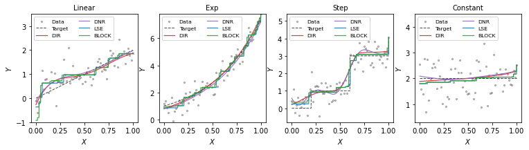
An illustration of PDIR is presented in Figure 1. In all subfigures, the data are depicted as grey dots, the underlying regression functions are plotted as solid black curves and PDIR estimates with different levels of penalty parameter are plotted as colored curves. In the top two figures, data are generated from models with monotonic regression functions. In the bottom left figure, the target function is a constant. In the bottom right figure, the model is misspecified, in which the underlying regression function is not monotonic. Small values of can lead to non-monotonic and reasonable estimates, suggesting that PDIR is robust against model misspecification. We have conducted more numerical experiments to evaluate the performance of PDIR, which indicates that PDIR tends to perform better than the existing isotonic regression methods considered in the comparison. The results are given in the Supplementary Material.
5.1 Non-asymptotic error bounds for PDIR
In this section, we state our main results on the bounds for the excess risk of the PDIR estimator defined in (13). Recall the definition of in (7). For notational simplicity, we write
| (14) |
The target function is the minimizer of risk over measurable functions, i.e., In isotonic regression, we assume that In addition, for any function , under the regression model (4), we have
We first state the conditions needed for establishing the excess risk bounds.
Assumption 17
(i) The target regression function defined in (4) is coordinate-wisely nondecreasing on , i.e., if for . (ii) The errors are independent and identically distributed noise variables with and , and ’s are independent of .
Assumption 17 includes basic model assumptions on the errors and the monotonic target function . In addition, we assume that the target function belongs to the class .
Next, we state the following basic lemma for bounding the excess risk.
Lemma 18 (Excess risk decomposition)
For the empirical risk minimizer defined in (13), its excess risk can be upper bounded by
The upper bound for the excess risk can be decomposed into two components: the stochastic error, given by the expected value of , and the approximation error, defined as . To establish a bound for the stochastic error, it is necessary to consider the complexities of both RePU networks and their derivatives, which have been investigated in our Theorem 1 and Lemma 2. To establish a bound for the approximation error , we rely on the simultaneous approximation results in Theorem 5.
Remark 19
The error decomposition in Lemma 18 differs from the canonical decomposition for score estimation in section 4.1, particularly pertaining to the stochastic error component. However, utilizing the decomposition in Lemma 18 enables us to derive a superior stochastic error bound by leveraging the properties of the PDIR loss function. A similar decomposition for least squares loss without penalization can be found in Jiao et al. (2023).
Lemma 20
Suppose that Assumptions 16, 17 hold and the target function defined in (4) belongs to for some . For any positive integer , let be the class of RePU activated neural networks with depth , width , number of neurons and size . Suppose that and . Then for , the excess risk of PDIR defined in (13) satisfies
| (15) | ||||
| (16) |
with
where the expectation is taken with respect to and , is the mean of the tuning parameters, is a universal constant and is a positive constant depending only on and the diameter of the support .
Lemma 20 establishes two error bounds for the PDIR estimator : (15) for the mean squared error between and the target , and (16) for controlling the non-monotonicity of via its partial derivatives with respect to a measure defined in terms of . Both bounds (15) and (16) are encompasses both stochastic and approximation errors. Specifically, the stochastic error is of order , which represents an improvement over the canonical error bound of , up to logarithmic factors in . This advancement is owing to the decomposition in Lemma 18 and the properties of PDIR loss function, which is different from traditional decomposition techniques.
Remark 21
In (16), the estimator is encouraged to exhibit monotonicity, as the expected monotonicity penalty on the estimator is bounded. Notably, when , the estimator is almost surely monotonic in its th argument with respect to the probability measure of . Based on (16), guarantees of the estimator’s monotonicity with respect to a single argument can be obtained. Specifically, for those where , we have , which provides a guarantee of the estimator’s monotonicity with respect to its th argument. Moreover, larger values of lead to smaller bounds, which is consistent with the intuition that larger values of better promote monotonicity of with respect to its th argument.
Theorem 22 (Non-asymptotic excess risk bounds)
By Theorem 22, our proposed PDIR estimator obtained with proper network architecture and tuning parameter achieves the minimax optimal rate up to logarithms for the nonparametric regression (Stone, 1982). Meanwhile, the PDIR estimator is guaranteed to be monotonic as measured by at a rate of up to a logarithmic factor.
Remark 23
In Theorem 22, we choose to attain the optimal rate of the expected mean squared error of up to a logarithmic factor. Additionally, we guarantee that the estimator to be monotonic at a rate of up to a logarithmic factor as measured by . The choice of is not unique for ensuring the consistency of . In fact, any choice of will result in a consistent . However, larger values of lead to a slower convergence rate of the expected mean squared error, but better guarantee for the monotonicity of .
The smoothness of the target function is unknown in practice and how to determine the smoothness of an unknown function is an important but nontrivial problem. Note that the convergence rate suffers from the curse of dimensionality since it can be extremely slow if is large.
High-dimensional data have low-dimensional latent structures in many applications. Below we show that PDIR can mitigate the curse of dimensionality if the data distribution is supported on an approximate low-dimensional manifold.
Lemma 24
Suppose that Assumptions 7, 16, 17 hold and the target function defined in (4) belongs to for some . Let be an integer with for some and universal constant . For any positive integer , let be the class of RePU activated neural networks with depth , width , number of neurons and size . Suppose that and . Then for , the excess risk of the PDIR estimator defined in (13) satisfies
| (17) | ||||
| (18) |
with
for where are universal constants and is a constant depending only on and the diameter of the support .
Based on Lemma 24, we obtain the following result.
Theorem 25 (Improved non-asymptotic excess risk bounds)
5.2 PDIR under model misspecification
In this subsection, we investigate PDIR under model misspecification when Assumption 17 (i) is not satisfied, meaning that the underlying regression function may not be monotonic.
Let be a random sample from model (4). Recall that the penalized risk of the deep isotonic regression is given by
If is not monotonic, the penalty is non-zero, and consequently, is not a minimizer of the risk when . Intuitively, the deep isotonic regression estimator will exhibit a bias towards the target due to the additional penalty terms in the risk. However, it is reasonable to expect that the estimator will have a smaller bias if are small. In the following lemma, we establish a non-asymptotic upper bound for our proposed deep isotonic regression estimator while adapting to model misspecification.
Lemma 26
Suppose that Assumptions 16 and 17 (ii) hold and the target function defined in (4) belongs to for some . For any positive integer let be the class of RePU activated neural networks with depth , width , number of neurons and size . Suppose that and . Then for , the excess risk of the PDIR estimator defined in (13) satisfies
| (19) | ||||
| (20) |
with
where the expectation is taken with respect to and , is the mean of the tuning parameters, is a universal constant and is a positive constant depending only on and the diameter of the support .
Lemma 26 is a generalized version of Lemma 20 for PDIR, as it holds regardless of whether the target function is isotonic or not. In Lemma 26, the expected mean squared error of the PDIR estimator can be bounded by three errors: stochastic error , approximation error , and misspecification error , without the monotonicity assumption. Compared with Lemma 20 with the monotonicity assumption, the approximation error is identical, the stochastic error is worse in terms of order, and the misspecification error appears as an extra term in the inequality. With an appropriate setup of for the neural network architecture with respect to the sample size , the stochastic error and approximation error can converge to zero, albeit at a slower rate than that in Theorem 22. However, the misspecification error remains constant for fixed tuning parameters . Thus, we can let the tuning parameters converge to zero to achieve consistency.
Remark 27
It is worth noting that if the target function is isotonic, then the misspecification error vanishes, leading the scenario to that of isotonic regression. However, the convergence rate based on Lemma 26 is slower than that in Lemma 20. The reason is that Lemma 26 is general and holds without prior knowledge of the monotonicity of the target function. If knowledge is available about the non-isotonicity of the th argument of the target function , setting the corresponding decreases the misspecification error and helps improve the upper bound.
Theorem 28 (Non-asymptotic excess risk bounds)
According to Lemma 26, under the misspecification model, the prediction error of PDIR attains its minimum when for , and the misspecification error vanishes. Consequently, the optimal convergence rate with respect to can be achieved by setting and for . It is worth noting that the prediction error of PDIR can achieve this rate as long as .
Remark 29
According to Theorem 28, there is no unique choice of that ensures the consistency of PDIR. Consistency is guaranteed even under a misspecified model when the for tend to zero as . Additionally, selecting a smaller value of provides a better upper bound for (19), and an optimal rate up to logarithms of can be achieved with a sufficiently small . An example demonstrating the effects of tuning parameters is visualized in the last subfigure of Figure 1.
6 Related works
In this section, we briefly review the papers in the existing literature that are most related to the present work.
6.1 ReLU and RePU networks
Deep learning has achieved impressive success in a wide range of applications. A fundamental reason for these successes is the ability of deep neural networks to approximate high-dimensional functions and extract effective data representations. There has been much effort devoted to studying the approximation properties of deep neural networks in recent years. Many interesting results have been obtained concerning the approximation power of deep neural networks for multivariate functions. Examples include Chen et al. (2019), Schmidt-Hieber (2020), Jiao et al. (2023). These works focused on the power of ReLU-activated neural networks for approximating various types of smooth functions.
For the approximation of the square function by ReLU networks, Yarotsky (2017) first used “sawtooth” functions, which achieves an error rate of with width 6 and depth for any positive integer . General construction of ReLU networks for approximating a square function can achieve an error with width and depth for any positive integers (Lu et al., 2021b). Based on this basic fact, the ReLU networks approximating multiplication and polynomials can be constructed correspondingly. However, the network complexity in terms of network size (depth and width) for a ReLU network to achieve precise approximation can be large compared to that of a RePU network since a RePU network can exactly compute polynomials with fewer layers and neurons.
The approximation results of the RePU network are generally obtained by converting splines or polynomials into RePU networks and making use of the approximation results of splines and polynomials. The universality of sigmoidal deep neural networks has been studied in the pioneering works (Mhaskar, 1993; Chui et al., 1994). In addition, the approximation properties of shallow Rectified Power Unit (RePU) activated network were studied in Klusowski and Barron (2018); Siegel and Xu (2022). The approximation rates of deep RePU neural networks on target functions in different spaces have also been explored, including Besov spaces (Ali and Nouy, 2021), Sobolev spaces (Li et al., 2019, 2020; Duan et al., 2021; Abdeljawad and Grohs, 2022) , and Hölder space (Belomestny et al., 2022). Most of the existing results on the expressiveness of neural networks measure the quality of approximation with respect to where norm. However, fewer papers have studied the approximation of derivatives of smooth functions (Duan et al., 2021; Gühring and Raslan, 2021; Belomestny et al., 2022).
6.2 Related works on score estimation
Learning a probability distribution from data is a fundamental task in statistics and machine learning for efficient generation of new samples from the learned distribution. Likelihood-based models approach this problem by directly learning the probability density function, but they have several limitations, such as an intractable normalizing constant and approximate maximum likelihood training.
One alternative approach to circumvent these limitations is to model the score function (Liu et al., 2016), which is the gradient of the logarithm of the probability density function. Score-based models can be learned using a variety of methods, including parametric score matching methods (Hyvärinen and Dayan, 2005; Sasaki et al., 2014), autoencoders as its denoising variants (Vincent, 2011), sliced score matching (Song et al., 2020), nonparametric score matching (Sriperumbudur et al., 2017; Sutherland et al., 2018), and kernel estimators based on Stein’s methods (Li and Turner, 2017; Shi et al., 2018). These score estimators have been applied in many research problems, such as gradient flow and optimal transport methods (Gao et al., 2019, 2022), gradient-free adaptive MCMC (Strathmann et al., 2015), learning implicit models (Warde-Farley and Bengio, 2016), inverse problems (Jalal et al., 2021). Score-based generative learning models, especially those using deep neural networks, have achieved state-of-the-art performance in many downstream tasks and applications, including image generation (Song and Ermon, 2019, 2020; Song et al., 2021; Ho et al., 2020; Dhariwal and Nichol, 2021; Ho et al., 2022), music generation (Mittal et al., 2021), and audio synthesis (Chen et al., 2020; Kong et al., 2020; Popov et al., 2021).
However, there is a lack of theoretical understanding of nonparametric score estimation using deep neural networks. The existing studies mainly considered kernel based methods. Zhou et al. (2020) studied regularized nonparametric score estimators using vector-valued reproducing kernel Hilbert space, which connects the kernel exponential family estimator (Sriperumbudur et al., 2017) with the score estimator based on Stein’s method (Li and Turner, 2017; Shi et al., 2018). Consistency and convergence rates of these kernel-based score estimator are also established under the correctly-specified model assumption in Zhou et al. (2020). For denoising autoencoders, Block et al. (2020) obtained generalization bounds for general nonparametric estimators also under the correctly-specified model assumption.
For sore-based learning using deep neural networks, the main difficulty for establishing the theoretical foundation is the lack of knowledge of differentiable neural networks since the derivatives of neural networks are involved in the estimation of score function. Previously, the non-differentiable Rectified Linear Unit (ReLU) activated deep neural network has received much attention due to its attractive properties in computation and optimization, and has been extensively studied in terms of its complexity (Bartlett et al., 1998; Anthony and Bartlett, 1999; Bartlett et al., 2019) and approximation power (Yarotsky, 2017; Petersen and Voigtlaender, 2018; Shen et al., 2020; Lu et al., 2021a; Jiao et al., 2023), based on which statistical learning theories for deep non-parametric estimations were established (Bauer and Kohler, 2019; Schmidt-Hieber, 2020; Jiao et al., 2023). For deep neural networks with differentiable activation functions, such as ReQU and RepU, the simultaneous approximation power on a smooth function and its derivatives were studied recently (Ali and Nouy, 2021; Belomestny et al., 2022; Siegel and Xu, 2022; Hon and Yang, 2022), but the statistical properties of differentiable networks are still largely unknown. To the best of our knowledge, the statistical learning theory has only been investigated for ReQU networks in Shen et al. (2022), where they have developed network representation of the derivatives of ReQU networks and studied their complexity.
6.3 Related works on isotonic regression
There is a rich and extensive literature on univariate isotonic regression, which is too vast to be adequately summarized here. So we refer to the books Barlow et al. (1972) and Robertson et al. (1988) for a systematic treatment of this topic and review of earlier works. For more recent developments on the error analysis of nonparametric isotonic regression, we refer to Durot (2002); Zhang (2002); Durot (2007, 2008); Groeneboom and Jongbloed (2014); Chatterjee et al. (2015), and Yang and Barber (2019), among others.
The least squares isotonic regression estimators under fixed design were extensively studied. With a fixed design at fixed points , the risk of the least squares estimator is defined by where the least squares estimator is defined by
| (21) |
The problem can be restated in terms of isotonic vector estimation on directed acyclic graphs. Specifically, the design points induce a directed acyclic graph with vertices and edges . The class of isotonic vectors on is defined by
Then the least squares estimation in (21) becomes that of searching for a target vector . The least squares estimator is actually the projection of onto the polyhedral convex cone (Han et al., 2019).
For univariate isotonic least squares regression with a bounded total variation target function , Zhang (2002) obtained sharp upper bounds for risk of the least squares estimator for . Shape-constrained estimators were also considered in different settings where automatic rate-adaptation phenomenon happens (Chatterjee et al., 2015; Gao et al., 2017; Bellec, 2018). We also refer to Kim et al. (2018); Chatterjee and Lafferty (2019) for other examples of adaptation in univariate shape-constrained problems.
Error analysis for the least squares estimator in multivariate isotonic regression is more difficult. For two-dimensional isotonic regression, where with and Gaussian noise, Chatterjee et al. (2018) considered the fixed lattice design case and obtained sharp error bounds. Han et al. (2019) extended the results of Chatterjee et al. (2018) to the case with , both from a worst-case perspective and an adaptation point of view. They also proved parallel results for random designs assuming the density of the covariate is bounded away from zero and infinity on the support.
Deng and Zhang (2020) considered a class of block estimators for multivariate isotonic regression in involving rectangular upper and lower sets under, which is defined as any estimator in-between the following max-min and min-max estimator. Under a -th moment condition on the noise, they developed risk bounds for such estimators for isotonic regression on graphs. Furthermore, the block estimator possesses an oracle property in variable selection: when depends on only an unknown set of variables, the risk of the block estimator automatically achieves the minimax rate up to a logarithmic factor based on the knowledge of the set of the variables.
Our proposed method and theoretical results are different from those in the aforementioned papers in several aspects. First, the resulting estimates from our method are smooth instead of piecewise constant as those based on the existing methods. Second, our method can mitigate the curse of dimensionality under an approximate low-dimensional manifold support assumption, which is weaker than the exact low-dimensional space assumption in the existing work. Finally, our method possesses a robustness property against model specification in the sense that it still yields consistent estimators if the monotonicity assumption is not strictly satisfied. However, the properties of the existing isotonic regression methods under model misspecification are unclear.
7 Conclusions
In this work, motivated by the problems of score estimation and isotonic regression, we have studied the properties of RePU-activated neural networks, including a novel generalization result for the derivatives of RePU networks and improved approximation error bounds for RePU networks with approximate low-dimensional structures. We have established non-asymptotic excess risk bounds for DSME, a deep score matching estimator; and PDIR, our proposed penalized deep isotonic regression method.
Our findings highlight the potential of RePU-activated neural networks in addressing challenging problems in machine learning and statistics. The ability to accurately represent the partial derivatives of RePU networks with RePUs mixed-activated networks is a valuable tool in many applications that require the use of neural network derivatives. Moreover, the improved approximation error bounds for RePU networks with low-dimensional structures demonstrate their potential to mitigate the curse of dimensionality in high-dimensional settings.
Future work can investigate further the properties of RePU networks, such as their stability, robustness, and interpretability. It would also be interesting to explore the use of RePU-activated neural networks in other applications, such as nonparametric variable selection and more general shape-constrained estimation problems. Additionally, our work can be extended to other smooth activation functions beyond RePUs, such as Gaussian error linear unit and scaled exponential linear unit, and study their derivatives and approximation properties.
Appendix
This appendix contains results from simulation studies to evaluate the performance of PDIR and proofs and supporting lemmas for the theoretical results stated in the paper.
Appendix A Numerical studies
In this section, we conduct simulation studies to evaluate the performance of PDIR and compare it with the existing isotonic regression methods. The methods included in the simulation include
-
•
The isotonic least squares estimator, denoted by Isotonic LSE, is defined as the minimizer of the mean square error on the training data subject to the monotone constraint. As the squared loss only involves the values at design points, then the isotonic LSE (with no more than linear constraints) can be computed with quadratic programming or using convex optimization algorithms (Dykstra, 1983; Kyng et al., 2015; Stout, 2015). Algorithmically, this turns out to be mappable to a network flow problem (Picard, 1976; Spouge et al., 2003). In our implementation, we compute Isotonic LSE via the Python package multiisotonic222https://github.com/alexfields/multiisotonic.
-
•
The block estimator (Deng and Zhang, 2020), denoted by Block estimator, is defined as any estimator between the block min-max and max-min estimators (Fokianos et al., 2020). In the simulation, we take the Block estimator as the mean of max-min and min-max estimators as suggested in (Deng and Zhang, 2020). The Isotonic LSE is shown to has an explicit mini-max representation on the design points for isotonic regression on graphs in general (Robertson et al., 1988). As in Deng and Zhang (2020), we use brute force which exhaustively calculates means over all blocks and finds the max-min value for each point . The computation cost via brute force is of order .
-
•
Deep isotonic regression estimator as described in Section 5, denoted by PDIR. Here we focus on using RePU activated network with . We implement it in Python via Pytorch and use Adam (Kingma and Ba, 2014) as the optimization algorithm with default learning rate 0.01 and default (coefficients used for computing running averages of gradients and their squares). The tuning parameters are chosen in the way that for .
-
•
Deep nonparametric regression estimator, denoted by DNR, which is actually the PDIR without penalty. The implementation is the same as that of PDIR, but the tuning parameters for .
A.1 Estimation and evaluation
For the proposed PDIR estimator, we set the tuning parameter for across the simulations. For each target function , according to model (4) we generate the training data with sample size and train the Isotonic LSE, Block estimator, PDIR and DNR estimators on . We would mention that the Block estimator has no definition when the input is “outside” the domain of training data , i.e., there exist no such that . In view of this, in our simulation we focus on using the training data with lattice design of the covariates for ease of presentation on the Block estimator. For PDIR and DNR estimators, such fixed lattice design of the covariates are not necessary and the obtained estimators can be smoothly extended to large domains which covers the domain of the training samples.
For each , we also generate the testing data with sample size from the same distribution of the training data. For the proposed method and for each obtained estimator , we calculate the mean squared error (MSE) on the testing data . We calculate the distance between the estimator and the corresponding target function on the testing data by
and we also calculate the distance between the estimator and the target function , i.e.
In the simulation studies, for each data generation model we generate testing data by the lattice points (100 even lattice points for each dimension of the input) where is the dimension of the input. We report the mean squared error, and distances to the target function defined above and their standard deviations over replications under different scenarios. The specific forms of are given in the data generation models below.
A.2 Univariate models
We consider three basic univariate models, including “Linear”, “Exp”, “Step”, “Constant” and “Wave”, which corresponds to different specifications of the target function . The formulae are given below.
-
(a)
Linear :
-
(b)
Exp:
-
(c)
Step:
-
(d)
Constant:
-
(e)
Wave:
where , and follows normal distribution. We use the linear model as a baseline model in our simulations and expect all the methods perform well under the linear model. The “Step” model is monotonic but not smooth even continuous. The “Constant” is a monotonic but not strictly monotonic model. And the “Wave” is a nonlinear, smooth but non monotonic model. These models are chosen so that we can evaluate the performance of Isotonic LSE, Block estimator PDIR and DNR under different types of models, including the conventional and misspecified cases.
For these models, we use the lattice design for the ease of presentation of Block estimator, where are the lattice points evenly distributed on interval . Figure S2 shows all these univariate data generation models.
Figures S3 shows an instance of the estimated curves for the “Linear”, “Exp”, “Step” and “Constant” models when sample size . In these plots, the training data is depicted as grey dots. The target functions are depicted as dashed curves in black, and the estimated functions are represented by solid curves with different colors. The summary statistics are presented in Table S3. Compared with the piece-wise constant estimates of Isotonic LSE and Block estimator, the PDIR estimator is smooth and it works reasonably well under univariate models, especially for models with smooth target functions.

| Model | Method | ||||||
|---|---|---|---|---|---|---|---|
| MSE | MSE | ||||||
| Linear | DNR | 0.266 (0.011) | 0.101 (0.035) | 0.122 (0.040) | 0.253 (0.011) | 0.055 (0.020) | 0.068 (0.023) |
| PDIR | 0.265 (0.012) | 0.098 (0.037) | 0.118 (0.041) | 0.254 (0.012) | 0.058 (0.024) | 0.070 (0.027) | |
| Isotonic LSE | 0.282 (0.013) | 0.140 (0.027) | 0.177 (0.035) | 0.262 (0.012) | 0.088 (0.012) | 0.113 (0.017) | |
| Block | 0.330 (0.137) | 0.165 (0.060) | 0.243 (0.155) | 0.277 (0.033) | 0.106 (0.021) | 0.153 (0.060) | |
| Exp | DNR | 0.268 (0.014) | 0.103 (0.043) | 0.124 (0.049) | 0.256 (0.012) | 0.055 (0.024) | 0.068 (0.027) |
| PDIR | 0.268 (0.017) | 0.102 (0.049) | 0.124 (0.056) | 0.255 (0.012) | 0.055 (0.022) | 0.068 (0.026) | |
| Isotonic LSE | 0.312 (0.018) | 0.195 (0.028) | 0.246 (0.034) | 0.274 (0.014) | 0.120 (0.014) | 0.153 (0.018) | |
| Block | 0.302 (0.021) | 0.177 (0.028) | 0.223 (0.034) | 0.272 (0.012) | 0.115 (0.015) | 0.146 (0.017) | |
| Step | DNR | 0.375 (0.045) | 0.259 (0.059) | 0.347 (0.061) | 0.315 (0.017) | 0.169 (0.022) | 0.253 (0.018) |
| PDIR | 0.366 (0.042) | 0.245 (0.058) | 0.335 (0.057) | 0.311 (0.018) | 0.153 (0.025) | 0.245 (0.018) | |
| Isotonic LSE | 0.304 (0.020) | 0.151 (0.041) | 0.228 (0.039) | 0.275 (0.014) | 0.081 (0.022) | 0.155 (0.020) | |
| Block | 0.382 (0.217) | 0.208 (0.082) | 0.327 (0.160) | 0.295 (0.046) | 0.108 (0.035) | 0.197 (0.086) | |
| Constant | DNR | 0.266 (0.012) | 0.102 (0.038) | 0.122 (0.042) | 0.258 (0.013) | 0.057 (0.021) | 0.069 (0.023) |
| PDIR | 0.260 (0.011) | 0.080 (0.045) | 0.092 (0.049) | 0.257 (0.012) | 0.051 (0.025) | 0.060 (0.028) | |
| Isotonic LSE | 0.265 (0.013) | 0.087 (0.044) | 0.114 (0.052) | 0.258 (0.012) | 0.044 (0.020) | 0.068 (0.025) | |
| Block | 0.264 (0.012) | 0.085 (0.044) | 0.108 (0.049) | 0.258 (0.012) | 0.044 (0.020) | 0.066 (0.025) | |
| Wave | DNR | 0.289 (0.023) | 0.156 (0.039) | 0.192 (0.044) | 0.262 (0.014) | 0.089 (0.025) | 0.110 (0.029) |
| PDIR | 0.530 (0.030) | 0.398 (0.026) | 0.528 (0.018) | 0.511 (0.022) | 0.368 (0.014) | 0.510 (0.009) | |
| Isotonic LSE | 0.525 (0.027) | 0.399 (0.022) | 0.524 (0.015) | 0.495 (0.020) | 0.353 (0.009) | 0.494 (0.004) | |
| Block | 0.516 (0.024) | 0.391 (0.022) | 0.519 (0.017) | 0.497 (0.023) | 0.358 (0.012) | 0.500 (0.013) | |
A.3 Bivariate models
We consider several basic multivariate models, including polynomial model (“Polynomial”), concave model (“Concave”), step model (“Step”), partial model (“Partial”), constant model (“Constant”) and wave model (“Wave”), which correspond to different specifications of the target function . The formulae are given below.
-
(a)
Polynomial:
-
(b)
Concave:
-
(c)
Step:
-
(d)
Partial:
-
(e)
Constant:
-
(f)
Wave:
where , , and follows normal distribution. The “Polynomial” and “Concave” models are monotonic models. The “Step” model is monotonic but not smooth even continuous. In “Partial ” model, the response is related to only one covariate. The “Constant” is a monotonic but not strictly monotonic model and the “Wave” is a nonlinear, smooth but non monotonic model. We use the lattice design for the ease of presentation of Block estimator, where are the lattice points evenly distributed on interval . Simulation results over 100 replications are summarized in Table S4. And for each model, we take an instance from the replications to present the heatmaps and the 3D surface of the predictions of these estimates; see Figure S4-S15. In heatmaps, we show the observed data (linearly interpolated), the true target function and the estimates of different methods. We can see that compared with the piece-wise constant estimates of Isotonic LSE and Block estimator, the DIR estimator is smooth and works reasonably well under bivariate models, especially for models with smooth target functions.
| Model | Method | ||||||
|---|---|---|---|---|---|---|---|
| MSE | MSE | ||||||
| Polynomial | DNR | 4.735 (0.344) | 0.138 (0.041) | 0.172 (0.046) | 4.655 (0.178) | 0.078 (0.022) | 0.098 (0.025) |
| PDIR | 4.724 (0.366) | 0.140 (0.045) | 0.171 (0.049) | 4.688 (0.181) | 0.077 (0.023) | 0.096 (0.026) | |
| Isotonic LSE | 8.309 (0.405) | 0.755 (0.061) | 0.884 (0.061) | 6.052 (0.153) | 0.364 (0.019) | 0.444 (0.021) | |
| Block | 4.780 (0.284) | 0.319 (0.020) | 0.397 (0.026) | 4.747 (0.129) | 0.210 (0.011) | 0.264 (0.017) | |
| Concave | DNR | 0.282 (0.016) | 0.142 (0.038) | 0.176 (0.042) | 0.261 (0.007) | 0.083 (0.022) | 0.103 (0.024) |
| PDIR | 0.276 (0.015) | 0.129 (0.038) | 0.158 (0.043) | 0.260 (0.007) | 0.077 (0.024) | 0.096 (0.028) | |
| Isotonic LSE | 0.393 (0.042) | 0.308 (0.051) | 0.375 (0.055) | 0.294 (0.010) | 0.163 (0.020) | 0.207 (0.022) | |
| Block | 0.303 (0.015) | 0.183 (0.025) | 0.229 (0.030) | 0.275 (0.006) | 0.125 (0.012) | 0.157 (0.014) | |
| Step | DNR | 0.561 (0.030) | 0.462 (0.020) | 0.557 (0.025) | 0.519 (0.011) | 0.432 (0.010) | 0.519 (0.010) |
| PDIR | 0.561 (0.030) | 0.461 (0.019) | 0.557 (0.024) | 0.519 (0.011) | 0.431 (0.010) | 0.520 (0.010) | |
| Isotonic LSE | 1.462 (0.104) | 0.852 (0.046) | 1.100 (0.047) | 0.700 (0.028) | 0.430 (0.019) | 0.672 (0.021) | |
| Block | 0.657 (0.031) | 0.503 (0.022) | 0.638 (0.023) | 0.461 (0.016) | 0.321 (0.014) | 0.457 (0.014) | |
| Partial | DNR | 12.67 (0.530) | 0.129 (0.033) | 0.161 (0.039) | 12.77 (0.338) | 0.079 (0.023) | 0.099 (0.027) |
| PDIR | 12.70 (0.548) | 0.112 (0.037) | 0.136 (0.042) | 12.72 (0.285) | 0.063 (0.021) | 0.080 (0.026) | |
| Isotonic LSE | 17.78 (0.532) | 0.739 (0.052) | 1.062 (0.055) | 15.00 (0.262) | 0.378 (0.024) | 0.528 (0.028) | |
| Block | 12.31 (0.571) | 0.435 (0.041) | 0.578 (0.043) | 12.50 (0.313) | 0.237 (0.028) | 0.313 (0.049) | |
| Constant | DNR | 0.278 (0.016) | 0.131 (0.038) | 0.160 (0.042) | 0.260 (0.005) | 0.079 (0.020) | 0.097 (0.022) |
| PDIR | 0.266 (0.013) | 0.094 (0.047) | 0.111 (0.050) | 0.255 (0.005) | 0.052 (0.022) | 0.063 (0.025) | |
| Isotonic LSE | 0.280 (0.021) | 0.121 (0.047) | 0.161 (0.056) | 0.262 (0.006) | 0.076 (0.025) | 0.108 (0.026) | |
| Block | 0.265 (0.012) | 0.089 (0.040) | 0.110 (0.046) | 0.256 (0.005) | 0.059 (0.022) | 0.075 (0.024) | |
| Wave | DNR | 0.306 (0.020) | 0.189 (0.036) | 0.233 (0.042) | 0.269 (0.009) | 0.108 (0.025) | 0.135 (0.029) |
| PDIR | 0.459 (0.058) | 0.390 (0.056) | 0.454 (0.063) | 0.581 (0.039) | 0.493 (0.028) | 0.574 (0.033) | |
| Isotonic LSE | 1.380 (0.085) | 0.918 (0.032) | 1.063 (0.040) | 0.989 (0.024) | 0.760 (0.014) | 0.860 (0.012) | |
| Block | 0.978 (0.022) | 0.750 (0.014) | 0.854 (0.012) | 0.892 (0.021) | 0.693 (0.009) | 0.802 (0.008) | |
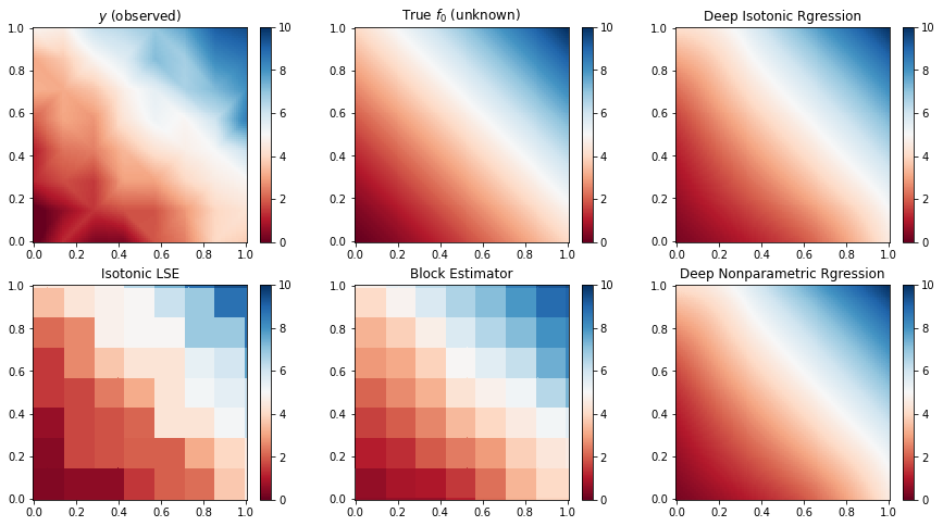


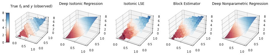


A.4 Tuning parameter
In this subsection, we investigate the numerical performance regrading to different choice of tuning parameters under different models.
For univariate models, we calculate the testing statistics and for tuning parameter on the 20 lattice points in the interval . For each , we simulate 20 times replications and reports the average , statistics and their 90% empirical band. For each replication, we train the PDIR using training samples and testing samples. In our simulation, four univariate models in section A.2 are considered including “Exp”, “Constant”, “Step” and misspecified model “Wave” and the results are reported in Figure S16. We can see that for isotonic models “Exp” and “Step”, the estimate is not sensitive to the choice of the tuning parameter in , which all leads to reasonable estimates. For “Constant” model, a not strictly isotonic model, errors slightly increase as the tuning parameter increases in . Overall, the choice can lead to reasonably well estimates for correctly specified models. For misspecified model “Wave”, the estimates deteriorates quickly as the tuning parameter increases around 0, and after that the additional negative effect of the increasing becomes slight.


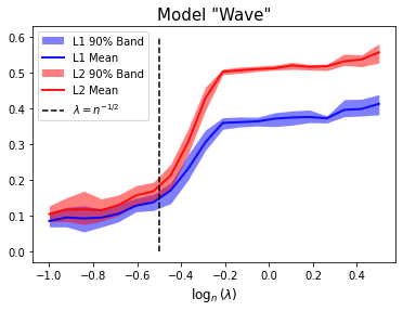
For bivariate models, our first simulation studies focus on the case where tuning parameters have the same value, i.e., . We calculate the testing statistics and for tuning parameters on the 20 lattice points in the interval . For each , we simulate 20 times replications and reports the average , statistics and their 90% empirical band. For each replication, we train the PDIR using training samples and testing samples. In our simulation, four bivariate models in section A.3 are considered including “Partial”, “Constant”, “Concave” and misspecified model “Wave” and the results are reported in Figure S17. The observation are similar to those of univariate models, that is, the estimates are not sensitive to the choices of tuning parameters over for correctly specified models, i.e., isotonic models. But for misspecified model “Wave”, the estimates deteriorates quickly as the tuning parameter increases around 0, and after that increasing slightly spoils the estimates.


In the second simulation study of bivariate models, we can choose different values for different components of the turning parameter , i.e., can be different from . We investigate this by considering the follow bivariate model, where the target function is monotonic in its second argument and non-monotonic in its first one.
-
Model (g)
:
where and follows normal distribution. Heatmaps for the observed training data, the target function , and 3D surface plots for the target function under model (g) when and are presented in Figure S18.
For model (g), we calculate the mean testing statistics and for tuning parameter on the 400 grid points on the region . For each , we simulate 5 times replications and reports the average , statistics. For each replication, we train the PDIR using training samples and testing samples. The mean and distance from the target function and the estimates on the testing data under different are depicted in Figure S19. We see that the target function is increasing in its second argument, and the estimates is insensitive to the tuning parameter , while the target function is non-monotonic in its first argument, and the estimates deteriorate when gets larger. The simulation results suggest that we should only penalize the gradient with respect to the monotonic arguments but not non-monotonic ones. The estimates is sensitive to the turning parameter for misspecified model, especially when the turning parameter increases around .


Appendix B Proofs
Proof of Theorem 1
For integer , let and denote the RePUs activation functions respectively. Let be vector of the width (number of neurons) of each layer in the original RePU network where and in our problem. We let be the function (subnetwork of the RePU network) from to which takes as input and outputs the -th neuron of the -th layer for and .
We construct Mixed RePUs activated subnetworks to compute iteratively for , i.e., we construct the partial derivatives of the original RePU subnetworks(up to -th layer) step by step. Without loss of generality, we compute for , and the construction is the same for all other . We illustrate the details of the construction of the Mixed RePUs subnetworks for the first two layers () and the last layer and apply induction for layers . Note that the derivative of RePU activation function is , then when for any ,
| (B.1) |
where we denote and by the corresponding weights and bias in -th layer of the original RePU network. Now we intend to construct a 4 layer (2 hidden layers) Mixed RePUs network with width which takes as input and outputs
Note that the output of such network contains all the quantities needed to calculated , and the process of construction can be continued iteratively and the induction proceeds. In the first hidden layer, we can obtain neurons
with weight matrix having parameters, bias vector and activation function vector being
where the first activation functions of are chosen to be , the last activation functions are chosen to be and the rest . In the second hidden layer, we can obtain neurons. The first neurons of the second hidden layer (or the third layer) are
which intends to implement identity map such that can be kept and outputted in the next layer since identity map can be realized by . The rest neurons of the second hidden layer (or the third layer) are
which is ready for implementing the multiplications in (B.1) to obtain since
In the second hidden layer (the third layer), the bias vector is zero , activation functions vector
and the corresponding weight matrix can be formulated correspondingly without difficulty which contains non-zero parameters. Then in the last layer, by the identity maps and multiplication operations with weight matrix having parameters, bias vector being zeros, we obtain
Such Mixed RePUs neural network has 2 hidden layers (4 layers), hidden neurons, parameters and its width is . It worth noting that the RePU activation functions do not apply to the last layer since the construction here is for a single network. When we are combining two consecutive subnetworks into one deep neural network, the RePU activation functions should apply to the last layer of the first subnetwork. Hence, in the construction of the whole big network, the last layer of the subnetwork here should output neurons
to keep in use in the next subnetwork. Then for this Mixed RePUs neural network, the weight matrix has parameters, the bias vector is zeros and the activation functions vector has all as elements. And such Mixed RePUs neural network has 2 hidden layers (4 layers), hidden neurons, parameters and its width is .
Now we consider the second step, for any ,
| (B.2) |
where and are defined correspondingly as the weights and bias in -th layer of the original RePU network. By the previous constructed subnetwork, we can start with its outputs
as the inputs of the second subnetwork we are going to build. In the first hidden layer of the second subnetwork, we can obtain neurons
with weight matrix having non-zero parameters, bias vector and activation functions vector . Similarly, the second hidden layer can be constructed to have neurons with weight matrix having non-zero parameters, zero bias vector and activation functions vector . The second hidden layer here serves exactly the same as that in the first subnetwork, which intends to implement the identity map for
and implement the multiplication in (B.2). Similarly, the last layer can also be constructed as that in the first subnetwork, which outputs
with the weight matrix having parameters, the bias vector being zeros and the activation functions vector with elements being . Then the second Mixed RePUs subnetwork has 2 hidden layers (4 layers), hidden neurons, parameters and its width is .
Then we can continuing this process of construction. For integers and for any ,
where and are defined correspondingly as the weights and bias in -th layer of the original RePU network. We can construct a Mixed RePUs network taking
as input, and it outputs
with 2 hidden layers, hidden neurons, parameters and its width is .
Iterate this process until the step, where the last layer of the original RePU network has only neurons. For the RePU activated neural network , the output of the network is a scalar and the partial derivative with respect to is
where and are the weights and bias parameter in the last layer of the original RePU network. The the constructed -th subnetwork taking
as input and it outputs which is the partial derivative of the whole RePU network with respect to its -th argument . The subnetwork should have 2 hidden layers width with hidden neurons, non-zero parameters.
Lastly, we combing all the subnetworks in order to form a big Mixed RePUs network which takes as input and outputs for . Recall that here are the depth, width, number of neurons and number of parameters of the original RePU network respectively, and we have and Then the big Mixed RePUs network has hidden layers (totally 3 layers), neurons, parameters and its width is . This completes the proof.
Proof of Lemma 2
We follow the idea of the proof of Theorem 6 in Bartlett et al. (2019) to prove a somewhat stronger result, where we give the upper bound of the Pseudo dimension of class of Mixed RePUs networks in terms of the depth, size and number of neurons of the network. Instead of the VC dimension of given in Bartlett et al. (2019), our Pseudo dimension bound is stronger since .
Let denote the domain of the functions and let , we consider a new class of functions
Then it is clear that and we next bound the VC dimension of . Recall that the the total number of parameters (weights and biases) in the neural network implementing functions in is , we let denote the parameters vector of the network implemented in . And here we intend to derive a bound for
which uniformly holds for all choice of and . Note that the maximum of over all all choice of and is just the growth function of . To give a uniform bound of , we use the Theorem 8.3 in Anthony and Bartlett (1999) as a main tool to deal with the analysis.
Lemma 30 (Theorem 8.3 in Anthony and Bartlett (1999))
Let be polynomials in variables of degree at most . If , define
i.e. is the number of possible sign vectors given by the polynomials. Then .
Now if we can find a partition of the parameter domain such that within each region , the functions are all fixed polynomials of bounded degree, then can be bounded via the following sum
| (B.3) |
and each term in this sum can be bounded via Lemma 30. Next, we construct the partition follows the same way as in Bartlett et al. (2019) iteratively layer by layer. We define the a sequence of successive refinements satisfying the following properties:
-
1.
The cardinality and for each ,
where denotes the number of neurons in the -th layer and denotes the total number of parameters (weights and biases) at the inputs to units in all the layers up to layer .
-
2.
For each , each element of of , each , and each unit in the -th layer, when varies in , the net input to is a fixed polynomial function in variables of , of total degree no more than where for each layer the activation functions are for some integer (this polynomial may depend on and ).
One can define , and it can be verified that satisfies property 2 above. Note that in our case, for fixed and and any subset , is a polynomial with respect to with degree the same as that of , which is no more than . Then the construction of and its verification for properties 1 and 2 can follow the same way in Bartlett et al. (2019). Finally we obtain a partition of such that for , the network output in response to any is a fixed polynomial of of degree no more than (since the last node just outputs its input). Then by Lemma 30
Besides, by property 1 we have
Then using (B.3), and since the sample are arbitrarily chosen, we have
where the second inequality follows from weighted arithmetic and geometric means inequality, the third holds since and the last holds since . Since is the growth function of , we have
where Since and , then by Lemma 16 in Bartlett et al. (2019) we have
Note that and , then we have
for some universal constant .
Proof of Theorem 3
We begin our proof with consider the simple case, which is to construct a proper RePU network to represent a univariate polynomial with no error. We can leverage Horner’s method or Qin Jiushao’s algorithm in China to construct such networks. Suppose is a univariate polynomial of degree , then it can be written as
We can iteratively calculate a sequence of intermediate variables by
Then we can obtain . By (iii) in Lemma 40, we know that a RePU network with one hidden layer and no more than nodes can represent any polynomial of the input with order no more than . Obviously, for input , the identity map , linear transformation and square map are all polynomials of with order no more than . In addition, it is not hard to see that the multiplication operator can be represented by a RePU network with one hidden layer and nodes. Then to calculate needs a RePU network with 1 hidden layer and hidden neurons, and to calculate needs a RePU network with 3 hidden layer, hidden neurons. By induction, to calculate for needs a RePU network with hidden layer, hidden neurons, parameters(weights and bias), and its width equals to .
Apart from the construction based on the Horner’s method, another construction is shown in Theorem 2 of li2019powernet, where the constructed RePU network has hidden layers, neurons and parameters (weights and bias).
Now we consider converting RePU networks to multivariate polynomial with total degree on . For any and , let
denote the polynomial with total degree of variables, where are non-negative integers, are coefficients in . Note that the multivariate polynomial can be written as
and we can view as a univariate polynomial of with degree if are given and for each the -variate polynomial with degree no more than can be computed by a proper RePU network. This reminds us the construction of RePU network for can be implemented recursively via composition of by induction.
By Horner’s method we have constructed a RePU network with hidden layers, hidden neurons and parameters to exactly compute . Now we start to show can be computed by RePU networks. We can write as
Note that for , the the degree of polynomial is which is less than . But we can still view it as a polynomial with degree by padding (adding zero terms) such that where if and if . In such a way, for each the polynomial can be computed by a RePU network with hidden layers, hidden neurons, parameters and its width equal to . Besides, for each , the monomial can also be computed by a RePU network with hidden layers, hidden neurons, parameters and its width equal to , in whose implementation the identity maps are used after the -th hidden layer. Now we parallel these two sub networks to get a RePU network which takes and as input and outputs with width , hidden layers , number of neurons and size . Since for each , such paralleled RePU network can be constructed, then with straightforward paralleling of such RePU networks, we obtain a RePU network exactly computes with width , hidden layers , number of neurons and number of parameters .
Similarly for polynomial of variables, we can write as
By our previous argument, for each , there exists a RePU network which takes as input and outputs with width , hidden layers , number of neurons and parameters . And by paralleling such subnetworks, we obtain a RePU network that exactly computes with width , hidden layers , number of neurons and number of parameters .
Continuing this process, we can construct RePU networks exactly compute polynomials of any variables with total degree . With a little bit abuse of notations, we let , , and denote the width, number of hidden layers, number of neurons and number of parameters (weights and bias) respectively of the RePU network computing for . We have known that
Besides, based on the iterate procedure of the network construction, by induction we can see that for the following equations hold,
Then based on the values of and the recursion formula, we have for
This completes our proof.
Proof of Theorem 5
The proof is straightforward by and leveraging the approximation power of multivariate polynomials based on Theorem 3. The theories for polynomial approximation have been extensively studies on various spaces of smooth functions. We refer to Bagby et al. (2002) for the polynomial approximation on smooth functions in our proof.
Lemma 31 (Theorem 2 in Bagby et al. (2002))
Let be a function of compact support on of class where and let be a compact subset of which contains the support of . Then for each nonnegative integer there is a polynomial of degree at most on with the following property: for each multi-index with we have
where is a positive constant depending only on and .
The proof of Lemma 31 can be found in Bagby et al. (2002) based on the Whitney extension theorem (Theorem 2.3.6 in Hörmander (2015)) and by examining the proof of Theorem 1 in Bagby et al. (2002), the dependence of the constant in Lemma 31 on the and can be detailed.
To use Lemma 31, we need to find a RePU network to compute the for each . By Theorem 3, we know that any of variables can be exactly computed by a RePU network with hidden layers, number of neurons, number of parameters (weights and bias) and network width . Then we have
where is a positive constant depending only on and . Note that the number neurons , which implies . Then we also have
where is a positive constant depending only on and . This completes the proof.
Proof of Theorem 8
The idea of our proof is based on projecting the data to a low-dimensional space and then use deep RePU neural network to approximate the low-dimensional function.
Given any integer satisfying , by Theorem 3.1 in Baraniuk and Wakin (2009) there exists a linear projector that maps a low-dimensional manifold in a high-dimensional space to a low-dimensional space nearly preserving the distance. Specifically, there exists a matrix such that where is an identity matrix of size , and
for any
Note that for any , there exists a unique such that . Then for any , define where is a set function which returns a unique element of a set. If where and , then by our argument since is a set with only one element when . We can see that is a differentiable function with the norm of its derivative locates in , since
for any . For the high-dimensional function , we define its low-dimensional representation by
Recall that , then . Note that is compact manifold and is a linear mapping, then by the extended version of Whitney’ extension theorem in Fefferman (2006), there exists a function such that for any and . By Theorem 5, for any , there exists a function implemented by a RePU network with its depth , width , number of neurons and size specified as
such that for each multi-index with , we have
for all where is a constant depending only on .
By Theorem 3, the linear projection can be computed by a RePU network with 1 hidden layer and its width no more than 18p. If we define which is for any , then is also a RePU network with one more layer than . For any , there exists a such that . Then, for each multi-index with , we have
where is a constant depending only on . The second last inequality follows from . Since the number neurons and , the last inequality follows. This completes the proof.
Proof of Lemma 10
For the empirical risk minimizer based on the sample , we consider its excess risk .
For any , we have
where the first inequality follows from the definition of empirical risk minimizer , and the second inequality holds since . Note that above inequality holds for any , then
where we call the stochastic error and the approximation error.
Bounding the stochastic error
Recall that are vector-valued functions, we write and let denote the -th diagonal entry in and the -th diagonal entry in .
Define
for and . Then,
| (B.4) |
Recall that for any , the output and the partial derivative for . Then by Theorem 11.8 in Mohri et al. (2018), for any , with probability at least over the choice of i.i.d sample ,
| (B.5) |
for where is the Pseudo dimension of and . Similarly, with probability at least over the choice of i.i.d sample ,
| (B.6) |
for where . Combining (B.4), (B.5) and (B.6), we have proved that for any , with probability at least ,
Note that for where is a class of RePU neural networks with depth , width , size and number of neurons . Then for each , the function class consists of RePU neural networks with depth , width , number of neurons and size no more than . By Lemma 2, we have . Similarly, by Theorem 1 and Lemma 2, we have . Then, for any , with probability at least
If we let , then above inequality implies
for . And
Bounding the approximation error
Recall that for ,
and the excess risk
Recall that and are vector-valued functions. For each , we let be a class of RePU neural networks with depth , width , size and number of neurons . Define . The neural networks in has depth , width , size and number of neurons , which can be seen as built by paralleling subnetworks in for . Let be the class of all RePU neural networks with depth , width , size and number of neurons . Then and
Now we focus on derive upper bound for
for each . By assumption, and for any . For each , the target defined on domain is a real-valued function belonging to class for . By Theorem 5, for any , there exists a RePU activated neural network with hidden layers, number of neurons, number of parameters and network width such that for each multi-index , we have ,
where is a positive constant depending only on and the diameter of . Then
holds for each . Sum up above inequalities, we have proved that
Non-asymptotic error bound
Based on the obtained stochastic error bound and approximation error bound, we can conclude that with probability at least , the empirical risk minimizer defined in (9) satisfies
and
where is a positive constant depending only on and the diameter of .
Note that the network depth is a positive odd number. Then we let be a positive odd number, and let the class of neuron network specified by depth , width , neurons and size . Then we can further express the stochastic error in term of :
where is a universal positive constant and is a positive constant depending only on and the diameter of .
Proof of Lemma 14
Proof of Lemma 18
Recall that is the empirical risk minimizer. Then, for any we have
For any , let
and
Then for any , we have and since and are nonnegative functions and ’s are nonnegative numbers. Note that by the assumption that is coordinate-wisely nondecreasing. Then,
We can then give upper bounds for the excess risk . For any ,
where the second inequality holds by the the fact that satisfies for any . Since the inequality holds for any , we have
This completes the proof.
Proof of Lemma 20
Proof of Lemma 24
Proof of Lemma 26
Under the misspecified model, the target function may not be monotonic, and the quantity is not guaranteed to be positive, which prevents us to use the decomposition technique in proof of Lemma 37 to get a fast rate. Instead, we use the canonical decomposition of the excess risk. Let be the sample, and let and . We notice that
and
where , denotes the expectation taken with respect to , and denotes the conditional expectation given . Then we have
where the first term is the stochastic error, the second term is the approximation error, and the third term the misspecification error with respect to the penalty. Compared with the decomposition in Lemma 18, the approximation error is the same and can be bounded using Lemma 38. However, the stochastic error is different, and there is an additional misspecification error. We will leave the misspecification error untouched and include it in the final upper bound. Next, we focus on deriving the upper bound for the stochastic error.
For and each and , let
Then we have
Recall that for any , the and by assumption for . By applying Theorem 11.8 in Mohri et al. (2018), for any , with probability at least over the choice of i.i.d sample ,
and
for where . Combining above in probability bounds, we know that for any , with probability at least ,
Recall that is a class of RePU neural networks with depth , width , size and number of neurons . By Lemma 2, Then for each , the function class consists of RePU neural networks with depth , width , number of neurons and size no more than . By Theorem 1 and Lemma 2, we have . Then, for any , with probability at least
If we let , then above inequality implies
for . And
Note that the network depth , number of neurons and number of parameters satisfies and . By Lemma 38, combining the error decomposition, we have
where is a universal constant, is a constant depending only on and the diameter of the support . This completes the proof.
Proof of Lemma 37
Let be the sample used to estimate from the distribution . And let be another sample independent of . Define
for any (random) and sample . It worth noting that for any and ,
since and for by assumption. For any and ,
since is a -Lipschitz function and and for for by assumption
Recall that the the empirical risk minimizer depends on the sample , and the stochastic error is
| (B.7) | ||||
| (B.8) |
In the following, we derive upper bounds of (B.7) and (B.8) respectively. For any random variable , it is clear that . In light of this, we aim at giving upper bounds for the tail probabilities
for . Given , for , we have
| (B.9) |
The bound the probability (B.9), we apply Lemma 24 in Shen et al. (2022). For completeness of the proof, we present Lemma in the following.
Lemma 32 (Lemma 24 in Shen et al. (2022))
Let be a set of functions with . Let be i.i.d. -valued random variables. Then for each and any and ,
where is the covering number of with radius under the norm . The definition of the covering number can be found in Appendix C.
Combining (B.9) and (B.10), for , we have
Choosing , we get
For any , by the definition of , it is easy to show . Then , which leads to
| (B.12) |
Similarly, combining (B.9) and (B.11), we can obtain
For any , by the definition of , it can be shown . Recall that for . Then where we view as if . This leads to
| (B.13) |
Then by Lemma 39 in Appendix C, we can further bound the covering number by the Pseudo dimension. More exactly, for and any , we have
and for for and any , we have
By Theorem 1 we know for . Combining the upper bounds of the covering numbers, we have
for and some universal constant where . By Lemma 2, for the function class implemented by Mixed RePU activated multilayer perceptrons with depth no more than , width no more than , number of neurons (nodes) no more than and size or number of parameters (weights and bias) no more than , we have
and by Lemma 2, for any function , its partial derivative can be implemented by a Mixed RePU activated multilayer perceptron with depth , width , number of neurons , number of parameters and bound . Then
It follows that
for and some universal constant . This completes the proof.
Proof of Lemma 38
Recall that
By Theorem 5, for each , there exists a RePU network with hidden layer, no more than neurons, no more than parameters and width no more than such that for each multi-index with we have
where is a positive constant depending only on and the diameter of . This implies
and for
Combine above two uniform bounds, we have
where is also a constant depending only on and . By defining the network depth to be a positive odd number, and expressing the network width , neurons and size in terms of , one can obtain the approximation error bound in terms of . This completes the proof.
Appendix C Definitions and Supporting Lemmas
C.1 Definitions
The following definitions are used in the proofs.
Definition 33 (Covering number)
Let be a class of function from to . For a given sequence let be the subset of . For a positive number , let be the covering number of under the norm with radius . Define the uniform covering number to be the maximum over all of the covering number , i.e.,
| (C.1) |
Definition 34 (Shattering)
Let be a family of functions from a set to . A set is said to be shattered by , if there exists such that
where is the sign function returns or and denotes the cardinality of a set. When they exist, the threshold values are said to witness the shattering.
Definition 35 (Pseudo dimension)
Let be a family of functions mapping from to . Then, the pseudo dimension of , denoted by , is the size of the largest set shattered by .
Definition 36 (VC dimension)
Let be a family of functions mapping from to . Then, the Vapnik–Chervonenkis (VC) dimension of , denoted by , is the size of the largest set shattered by with all threshold values being zero, i.e., .
C.2 Supporting Lemmas
Lemma 37 (Stochastic error bound)
Suppose Assumption 16 and 17 hold. Let be the RePU activated multilayer perceptron and let denote the class of the partial derivative of with respect to its first argument. Then for , the stochastic error satisfies
for some universal constant where .
Lemma 38 (Approximation error bound)
Suppose that the target function defined in (4) belongs to for some . For any positive odd number , let be the class of RePU activated neural networks with depth , width , number of neurons and size , satisfying and . Then the approximation error given in Lemma 18 satisfies
where , is the Lipschitz constant of the panelty function and is a constant depending only on and the diameter of the support .
The following lemma gives an upper bound for the covering number in terms of the pseudo-dimension.
Lemma 39 (Theorem 12.2 in Anthony and Bartlett (1999))
Let be a set of real functions from domain to the bounded interval . Let and suppose that has finite pseudo-dimension then
which is less than for .
The following lemma presents basic approximation properties of RePU network on monomials.
Lemma 40 (Lemma 1 in li2019powernet)
The monomials can be exactly represented by RePU () activated neural network with one hidden layer and no more than nodes. More exactly,
-
(i)
If , the monomial can be computed by a RePU activated network with one hidden layer and 1 nodes as
-
(ii)
If , the monomial can be computed by a RePU activated network with one hidden layer and 2 nodes as
-
(iii)
If , the monomial can be computed by a RePU activated network with one hidden layer and no more than nodes. More generally, a polynomial of degree no more than , i.e. , can also be computed by a RePU activated network with one hidden layer and no more than nodes as
where
Here are distinct values in and values of satisfy the linear system
where are binomial coefficients. Note that the top-left sub-matrix of the matrix above is a Vandermonde matrix, which is invertible as long as are distinct.
References
- Abdeljawad and Grohs (2022) Ahmed Abdeljawad and Philipp Grohs. Approximations with deep neural networks in sobolev time-space. Analysis and Applications, 20(03):499–541, 2022.
- Ali and Nouy (2021) Mazen Ali and Anthony Nouy. Approximation of smoothness classes by deep rectifier networks. SIAM Journal on Numerical Analysis, 59(6):3032–3051, 2021.
- Anthony and Bartlett (1999) Martin Anthony and Peter L. Bartlett. Neural Network Learning: Theoretical Foundations. Cambridge University Press, Cambridge, 1999. ISBN 0-521-57353-X. doi: 10.1017/CBO9780511624216. URL https://doi.org/10.1017/CBO9780511624216.
- Bagby et al. (2002) Thomas Bagby, Len Bos, and Norman Levenberg. Multivariate simultaneous approximation. Constructive approximation, 18(4):569–577, 2002.
- Baraniuk and Wakin (2009) Richard G. Baraniuk and Michael B. Wakin. Random projections of smooth manifolds. Found. Comput. Math., 9(1):51–77, 2009. ISSN 1615-3375. doi: 10.1007/s10208-007-9011-z. URL https://doi.org/10.1007/s10208-007-9011-z.
- Barlow et al. (1972) R. E. Barlow, D. J. Bartholomew, J. M. Bremner, and H. D. Brunk. Statistical Inference under Order Restrictions; the Theory and Application of Isotonic Regression. New York: Wiley, 1972.
- Bartlett et al. (1998) Peter Bartlett, Vitaly Maiorov, and Ron Meir. Almost linear vc dimension bounds for piecewise polynomial networks. Advances in neural information processing systems, 11, 1998.
- Bartlett et al. (2017) Peter L Bartlett, Dylan J Foster, and Matus J Telgarsky. Spectrally-normalized margin bounds for neural networks. In I. Guyon, U. Von Luxburg, S. Bengio, H. Wallach, R. Fergus, S. Vishwanathan, and R. Garnett, editors, Advances in Neural Information Processing Systems, volume 30. Curran Associates, Inc., 2017. URL https://proceedings.neurips.cc/paper_files/paper/2017/file/b22b257ad0519d4500539da3c8bcf4dd-Paper.pdf.
- Bartlett et al. (2019) Peter L. Bartlett, Nick Harvey, Christopher Liaw, and Abbas Mehrabian. Nearly-tight VC-dimension and pseudodimension bounds for piecewise linear neural networks. Journal of Machine Learning Research, 20:Paper No. 63, 17, 2019. ISSN 1532-4435.
- Bauer and Kohler (2019) Benedikt Bauer and Michael Kohler. On deep learning as a remedy for the curse of dimensionality in nonparametric regression. Ann. Statist., 47(4):2261–2285, 2019. ISSN 0090-5364. doi: 10.1214/18-AOS1747. URL https://doi.org/10.1214/18-AOS1747.
- Belkin and Niyogi (2003) Mikhail Belkin and Partha Niyogi. Laplacian eigenmaps for dimensionality reduction and data representation. Neural Comput., 15(6):1373–1396, 2003.
- Bellec (2018) Pierre C Bellec. Sharp oracle inequalities for least squares estimators in shape restricted regression. The Annals of Statistics, 46(2):745–780, 2018.
- Belomestny et al. (2022) Denis Belomestny, Alexey Naumov, Nikita Puchkin, and Sergey Samsonov. Simultaneous approximation of a smooth function and its derivatives by deep neural networks with piecewise-polynomial activations. arXiv:2206.09527, 2022.
- Block et al. (2020) Adam Block, Youssef Mroueh, and Alexander Rakhlin. Generative modeling with denoising auto-encoders and langevin sampling. arXiv:2002.00107, 2020.
- Chatterjee and Lafferty (2019) Sabyasachi Chatterjee and John Lafferty. Adaptive risk bounds in unimodal regression. Bernoulli, 25(1):1–25, 2019.
- Chatterjee et al. (2015) Sabyasachi Chatterjee, Adityanand Guntuboyina, and Bodhisattva Sen. On risk bounds in isotonic and other shape restricted regression problems. The Annals of Statistics, 43(4):1774–1800, 2015.
- Chatterjee et al. (2018) Sabyasachi Chatterjee, Adityanand Guntuboyina, and Bodhisattva Sen. On matrix estimation under monotonicity constraints. Bernoulli, 24(2):1072–1100, 2018.
- Chen et al. (2019) Minshuo Chen, Haoming Jiang, and Tuo Zhao. Efficient approximation of deep relu networks for functions on low dimensional manifolds. Advances in Neural Information Processing Systems, 2019.
- Chen et al. (2022) Minshuo Chen, Haoming Jiang, Wenjing Liao, and Tuo Zhao. Nonparametric regression on low-dimensional manifolds using deep relu networks: Function approximation and statistical recovery. Information and Inference: A Journal of the IMA, 11(4):1203–1253, 2022.
- Chen et al. (2020) Nanxin Chen, Yu Zhang, Heiga Zen, Ron J Weiss, Mohammad Norouzi, and William Chan. Wavegrad: Estimating gradients for waveform generation. arXiv:2009.00713, 2020.
- Chui and Li (1993) Charles K Chui and Xin Li. Realization of neural networks with one hidden layer. In Multivariate approximation: From CAGD to wavelets, pages 77–89. World Scientific, 1993.
- Chui et al. (1994) Charles K Chui, Xin Li, and Hrushikesh Narhar Mhaskar. Neural networks for localized approximation. mathematics of computation, 63(208):607–623, 1994.
- Deng and Zhang (2020) Hang Deng and Cun-Hui Zhang. Isotonic regression in multi-dimensional spaces and graphs. The Annals of Statistics, 48(6):3672–3698, 2020.
- Dhariwal and Nichol (2021) Prafulla Dhariwal and Alexander Nichol. Diffusion models beat gans on image synthesis. Advances in Neural Information Processing Systems, 34:8780–8794, 2021.
- Diggle et al. (1999) Peter Diggle, Sara Morris, and Tony Morton-Jones. Case-control isotonic regression for investigation of elevation in risk around a point source. Statistics in medicine, 18(13):1605–1613, 1999.
- Duan et al. (2021) Chenguang Duan, Yuling Jiao, Yanming Lai, Xiliang Lu, and Zhijian Yang. Convergence rate analysis for deep ritz method. arXiv preprint arXiv:2103.13330, 2021.
- Durot (2002) Cécile Durot. Sharp asymptotics for isotonic regression. Probability theory and related fields, 122(2):222–240, 2002.
- Durot (2007) Cécile Durot. On the -error of monotonicity constrained estimators. The Annals of Statistics, 35(3):1080–1104, 2007.
- Durot (2008) Cécile Durot. Monotone nonparametric regression with random design. Mathematical methods of statistics, 17(4):327–341, 2008.
- Dykstra (1983) Richard L Dykstra. An algorithm for restricted least squares regression. Journal of the American Statistical Association, 78(384):837–842, 1983.
- Fefferman (2006) Charles Fefferman. Whitney’s extension problem for . Annals of Mathematics., 164(1):313–359, 2006. ISSN 0003486X. URL http://www.jstor.org/stable/20159991.
- Fefferman et al. (2016) Charles Fefferman, Sanjoy Mitter, and Hariharan Narayanan. Testing the manifold hypothesis. Journal of the American Mathematical Society, 29(4):983–1049, 2016.
- Fokianos et al. (2020) Konstantinos Fokianos, Anne Leucht, and Michael H Neumann. On integrated convergence rate of an isotonic regression estimator for multivariate observations. IEEE Transactions on Information Theory, 66(10):6389–6402, 2020.
- Gao et al. (2017) Chao Gao, Fang Han, and Cun-Hui Zhang. Minimax risk bounds for piecewise constant models. arXiv preprint arXiv:1705.06386, 2017.
- Gao et al. (2019) Yuan Gao, Yuling Jiao, Yang Wang, Yao Wang, Can Yang, and Shunkang Zhang. Deep generative learning via variational gradient flow. In International Conference on Machine Learning, pages 2093–2101. PMLR, 2019.
- Gao et al. (2022) Yuan Gao, Jian Huang, Yuling Jiao, Jin Liu, Xiliang Lu, and Zhijian Yang. Deep generative learning via euler particle transport. In Mathematical and Scientific Machine Learning, pages 336–368. PMLR, 2022.
- Groeneboom and Jongbloed (2014) Piet Groeneboom and Geurt Jongbloed. Nonparametric estimation under shape constraints, volume 38. Cambridge University Press, 2014.
- Gühring and Raslan (2021) Ingo Gühring and Mones Raslan. Approximation rates for neural networks with encodable weights in smoothness spaces. Neural Networks, 134:107–130, 2021.
- Han et al. (2019) Qiyang Han, Tengyao Wang, Sabyasachi Chatterjee, and Richard J Samworth. Isotonic regression in general dimensions. The Annals of Statistics, 47(5):2440–2471, 2019.
- Ho et al. (2020) Jonathan Ho, Ajay Jain, and Pieter Abbeel. Denoising diffusion probabilistic models. Advances in Neural Information Processing Systems, 33:6840–6851, 2020.
- Ho et al. (2022) Jonathan Ho, Chitwan Saharia, William Chan, David J Fleet, Mohammad Norouzi, and Tim Salimans. Cascaded diffusion models for high fidelity image generation. J. Mach. Learn. Res., 23:47–1, 2022.
- Hoffmann et al. (2009) Heiko Hoffmann, Stefan Schaal, and Sethu Vijayakumar. Local dimensionality reduction for non-parametric regression. Neural Processing Letters, 29(2):109, 2009.
- Hon and Yang (2022) Sean Hon and Haizhao Yang. Simultaneous neural network approximation for smooth functions. Neural Networks, 154:152–164, 2022.
- Hörmander (2015) Lars Hörmander. The analysis of linear partial differential operators I: Distribution theory and Fourier analysis. Springer, 2015.
- Horner (1819) William George Horner. A new method of solving numerical equations of all orders, by continuous approximation. Philosophical Transactions of the Royal Society of London, (109):308–335, 1819.
- Horowitz and Lee (2017) Joel L Horowitz and Sokbae Lee. Nonparametric estimation and inference under shape restrictions. Journal of Econometrics, 201(1):108–126, 2017.
- Hyvärinen and Dayan (2005) Aapo Hyvärinen and Peter Dayan. Estimation of non-normalized statistical models by score matching. Journal of Machine Learning Research, 6(4), 2005.
- Jalal et al. (2021) Ajil Jalal, Marius Arvinte, Giannis Daras, Eric Price, Alexandros G Dimakis, and Jon Tamir. Robust compressed sensing mri with deep generative priors. Advances in Neural Information Processing Systems, 34:14938–14954, 2021.
- Jiang et al. (2011) Xiaoqian Jiang, Melanie Osl, Jihoon Kim, and Lucila Ohno-Machado. Smooth isotonic regression: A new method to calibrate predictive models. AMIA Summits on Translational Science Proceedings, 2011:16, 2011.
- Jiao et al. (2023) Yuling Jiao, Guohao Shen, Yuanyuan Lin, and Jian Huang. Deep nonparametric regression on approximate manifolds: Nonasymptotic error bounds with polynomial prefactors. The Annals of Statistics, 51(2):691–716, 2023.
- Kim et al. (2018) Arlene KH Kim, Adityanand Guntuboyina, and Richard J Samworth. Adaptation in log-concave density estimation. The Annals of Statistics, 46(5):2279–2306, 2018.
- Kingma and Ba (2014) Diederik P Kingma and Jimmy Ba. Adam: A method for stochastic optimization. arXiv preprint arXiv:1412.6980, 2014.
- Klusowski and Barron (2018) Jason M Klusowski and Andrew R Barron. Approximation by combinations of relu and squared relu ridge functions with and controls. IEEE Transactions on Information Theory, 64(12):7649–7656, 2018.
- Kong et al. (2020) Zhifeng Kong, Wei Ping, Jiaji Huang, Kexin Zhao, and Bryan Catanzaro. Diffwave: A versatile diffusion model for audio synthesis. arXiv:2009.09761, 2020.
- Kyng et al. (2015) Rasmus Kyng, Anup Rao, and Sushant Sachdeva. Fast, provable algorithms for isotonic regression in all l_p-norms. Advances in neural information processing systems, 28, 2015.
- Lee et al. (2022) Holden Lee, Jianfeng Lu, and Yixin Tan. Convergence for score-based generative modeling with polynomial complexity. arXiv:2206.06227, 2022.
- Li et al. (2019) Bo Li, Shanshan Tang, and Haijun Yu. Better approximations of high dimensional smooth functions by deep neural networks with rectified power units. arXiv preprint arXiv:1903.05858, 2019.
- Li et al. (2020) Bo Li, Shanshan Tang, and Haijun Yu. Powernet: Efficient representations of polynomials and smooth functions by deep neural networks with rectified power units. J. Math. Study, 53(2):159–191, 2020.
- Li and Turner (2017) Yingzhen Li and Richard E Turner. Gradient estimators for implicit models. arXiv:1705.07107, 2017.
- Liu et al. (2016) Qiang Liu, Jason Lee, and Michael Jordan. A kernelized stein discrepancy for goodness-of-fit tests. In International conference on machine learning, pages 276–284. PMLR, 2016.
- Lu et al. (2021a) Jianfeng Lu, Zuowei Shen, Haizhao Yang, and Shijun Zhang. Deep network approximation for smooth functions. SIAM Journal on Mathematical Analysis, 53(5):5465–5506, 2021a.
- Lu et al. (2021b) Jianfeng Lu, Zuowei Shen, Haizhao Yang, and Shijun Zhang. Deep network approximation for smooth functions. SIAM Journal on Mathematical Analysis, 53(5):5465–5506, 2021b.
- Luss et al. (2012) Ronny Luss, Saharon Rosset, and Moni Shahar. Efficient regularized isotonic regression with application to gene–gene interaction search. The Annals of Applied Statistics, 6(1):253–283, 2012.
- Mhaskar (1993) Hrushikesh Narhar Mhaskar. Approximation properties of a multilayered feedforward artificial neural network. Advances in Computational Mathematics, 1(1):61–80, 1993.
- Mittal et al. (2021) Gautam Mittal, Jesse Engel, Curtis Hawthorne, and Ian Simon. Symbolic music generation with diffusion models. arXiv:2103.16091, 2021.
- Mohri et al. (2018) Mehryar Mohri, Afshin Rostamizadeh, and Ameet Talwalkar. Foundations of machine learning. MIT press, 2018.
- Morton-Jones et al. (2000) Tony Morton-Jones, Peter Diggle, Louise Parker, Heather O Dickinson, and Keith Binks. Additive isotonic regression models in epidemiology. Statistics in medicine, 19(6):849–859, 2000.
- Nagarajan and Kolter (2019) Vaishnavh Nagarajan and J Zico Kolter. Deterministic pac-bayesian generalization bounds for deep networks via generalizing noise-resilience. arXiv preprint arXiv:1905.13344, 2019.
- Neyshabur et al. (2015) Behnam Neyshabur, Ryota Tomioka, and Nathan Srebro. Norm-based capacity control in neural networks. In Conference on learning theory, pages 1376–1401. PMLR, 2015.
- Petersen and Voigtlaender (2018) Philipp Petersen and Felix Voigtlaender. Optimal approximation of piecewise smooth functions using deep relu neural networks. Neural Networks, 108:296–330, 2018.
- Picard (1976) Jean-Claude Picard. Maximal closure of a graph and applications to combinatorial problems. Management science, 22(11):1268–1272, 1976.
- Popov et al. (2021) Vadim Popov, Ivan Vovk, Vladimir Gogoryan, Tasnima Sadekova, and Mikhail Kudinov. Grad-tts: A diffusion probabilistic model for text-to-speech. In International Conference on Machine Learning, pages 8599–8608. PMLR, 2021.
- Qin et al. (2014) Jing Qin, Tanya P Garcia, Yanyuan Ma, Ming-Xin Tang, Karen Marder, and Yuanjia Wang. Combining isotonic regression and em algorithm to predict genetic risk under monotonicity constraint. The annals of applied statistics, 8(2):1182, 2014.
- Robertson et al. (1988) T. Robertson, F. T. Wright, and R. L. Dykstra. Order Restricted Statistical Inference. New York: Wiley, 1988.
- Rueda et al. (2009) Cristina Rueda, Miguel A Fernández, and Shyamal Das Peddada. Estimation of parameters subject to order restrictions on a circle with application to estimation of phase angles of cell cycle genes. Journal of the American Statistical Association, 104(485):338–347, 2009.
- Sasaki et al. (2014) Hiroaki Sasaki, Aapo Hyvärinen, and Masashi Sugiyama. Clustering via mode seeking by direct estimation of the gradient of a log-density. In Joint European Conference on Machine Learning and Knowledge Discovery in Databases, pages 19–34. Springer, 2014.
- Schmidt-Hieber (2019) Johannes Schmidt-Hieber. Deep relu network approximation of functions on a manifold. arXiv:1908.00695, 2019.
- Schmidt-Hieber (2020) Johannes Schmidt-Hieber. Nonparametric regression using deep neural networks with ReLU activation function. Annals of Statistics, 48(4):1875–1897, 2020.
- Shen et al. (2022) Guohao Shen, Yuling Jiao, Yuanyuan Lin, Joel L Horowitz, and Jian Huang. Estimation of non-crossing quantile regression process with deep requ neural networks. arXiv:2207.10442, 2022.
- Shen et al. (2020) Zuowei Shen, Haizhao Yang, and Shijun Zhang. Deep network approximation characterized by number of neurons. Commun. Comput. Phys., 28(5):1768–1811, 2020. ISSN 1815-2406. doi: 10.4208/cicp.oa-2020-0149. URL https://doi.org/10.4208/cicp.oa-2020-0149.
- Shi et al. (2018) Jiaxin Shi, Shengyang Sun, and Jun Zhu. A spectral approach to gradient estimation for implicit distributions. In International Conference on Machine Learning, pages 4644–4653. PMLR, 2018.
- Siegel and Xu (2022) Jonathan W Siegel and Jinchao Xu. High-order approximation rates for shallow neural networks with cosine and reluk activation functions. Applied and Computational Harmonic Analysis, 58:1–26, 2022.
- Song and Ermon (2019) Yang Song and Stefano Ermon. Generative modeling by estimating gradients of the data distribution. Advances in Neural Information Processing Systems, 32, 2019.
- Song and Ermon (2020) Yang Song and Stefano Ermon. Improved techniques for training score-based generative models. Advances in neural information processing systems, 33:12438–12448, 2020.
- Song et al. (2020) Yang Song, Sahaj Garg, Jiaxin Shi, and Stefano Ermon. Sliced score matching: A scalable approach to density and score estimation. In Uncertainty in Artificial Intelligence, pages 574–584. PMLR, 2020.
- Song et al. (2021) Yang Song, Jascha Sohl-Dickstein, Diederik P Kingma, Abhishek Kumar, Stefano Ermon, and Ben Poole. Score-based generative modeling through stochastic differential equations. In International Conference on Learning Representations, 2021. URL https://openreview.net/forum?id=PxTIG12RRHS.
- Spouge et al. (2003) J Spouge, H Wan, and WJ Wilbur. Least squares isotonic regression in two dimensions. Journal of Optimization Theory and Applications, 117(3):585–605, 2003.
- Sriperumbudur et al. (2017) Bharath Sriperumbudur, Kenji Fukumizu, Arthur Gretton, Aapo Hyvärinen, and Revant Kumar. Density estimation in infinite dimensional exponential families. Journal of Machine Learning Research, 2017.
- Stone (1982) Charles J Stone. Optimal global rates of convergence for nonparametric regression. The annals of statistics, pages 1040–1053, 1982.
- Stout (2015) Quentin F Stout. Isotonic regression for multiple independent variables. Algorithmica, 71(2):450–470, 2015.
- Strathmann et al. (2015) Heiko Strathmann, Dino Sejdinovic, Samuel Livingstone, Zoltan Szabo, and Arthur Gretton. Gradient-free hamiltonian monte carlo with efficient kernel exponential families. Advances in Neural Information Processing Systems, 28, 2015.
- Sutherland et al. (2018) Danica J Sutherland, Heiko Strathmann, Michael Arbel, and Arthur Gretton. Efficient and principled score estimation with nyström kernel exponential families. In International Conference on Artificial Intelligence and Statistics, pages 652–660. PMLR, 2018.
- Vincent (2011) Pascal Vincent. A connection between score matching and denoising autoencoders. Neural computation, 23(7):1661–1674, 2011.
- Warde-Farley and Bengio (2016) David Warde-Farley and Yoshua Bengio. Improving generative adversarial networks with denoising feature matching. 2016.
- Wei and Ma (2019) Colin Wei and Tengyu Ma. Data-dependent sample complexity of deep neural networks via lipschitz augmentation. Advances in Neural Information Processing Systems, 32, 2019.
- Xu and Cao (2005) Zong-Ben Xu and Fei-Long Cao. Simultaneous lp-approximation order for neural networks. Neural Networks, 18(7):914–923, 2005.
- Yang and Barber (2019) Fan Yang and Rina Foygel Barber. Contraction and uniform convergence of isotonic regression. Electronic Journal of Statistics, 13(1):646–677, 2019.
- Yarotsky (2017) Dmitry Yarotsky. Error bounds for approximations with deep ReLU networks. Neural Networks, 94:103–114, 2017.
- Yarotsky (2018) Dmitry Yarotsky. Optimal approximation of continuous functions by very deep ReLU networks. In Conference on Learning Theory, pages 639–649. PMLR, 2018.
- Zhang (2002) Cun-Hui Zhang. Risk bounds in isotonic regression. The Annals of Statistics, 30(2):528–555, 2002.
- Zhou et al. (2020) Yuhao Zhou, Jiaxin Shi, and Jun Zhu. Nonparametric score estimators. In International Conference on Machine Learning, pages 11513–11522. PMLR, 2020.