DiffCPS: Diffusion-based Constrained Policy Search for Offline Reinforcement Learning

Consider a Markov decision process (MDP): $M=\{{\mathcal{S}},{\mathcal{A}},P,R,\gamma,d_{0}\}$, with state space $S$, action space ${\mathcal{A}}$, environment dynamics ${\mathcal{P}}({\bm{s}}^{\prime}|{\bm{s}},{\bm{a}}):S\times S\times{\mathcal{A}}\rightarrow[0,1]$, reward function $R:S\times{\mathcal{A}}\rightarrow{\mathbb{R}}$, discount factor $\gamma\in[0,1)$, policy $\mu\in{\mathcal{P}}({\mathcal{S}})$, where ${\mathcal{P}}({\mathcal{S}})$ is the space of probability measures on $({\mathcal{A}},{\mathcal{B}}({\mathcal{A}}))$ parametrized by elements of ${\mathcal{S}}$, where ${\mathcal{B}}({\mathcal{A}})$ are the Borel sets of ${\mathcal{A}}$, and initial state distribution $d_{0}$. The action-value or Q-value of policy $\mu$ is defined as $Q^{\mu}({\bm{s}}_{t},{\bm{a}}_{t})=\mathbb{E}_{{\bm{a}}_{t+1},{\bm{a}}_{t+2},...\sim\mu}\left[\sum_{j=0}^{\infty}\gamma^{j}r({\bm{s}}_{t+j},{\bm{a}}_{t+j})\right]$. Our goal is to get a policy to maximize the cumulative discounted reward $J(\theta)=\int_{\mathcal{S}}d_{0}({\bm{s}})Q^{\mu}({\bm{s}},{\bm{a}})d{\bm{s}}$, where $\rho^{\mu}({\bm{s}})=(1-\gamma)\sum_{t=0}^{\infty}\gamma^{t}p_{\mu}({\bm{s}}_{t}={\bm{s}})$ is the normalized discounted state visitation frequencies induced by the policy $\mu$ and $p_{\mu}({\bm{s}}_{t}={\bm{s}})$ is the likelihood of the policy being in state ${\bm{s}}$ after following $\mu$ for $t$ timesteps (Sutton & Barto, 2018; Peng et al., 2019).

In offline setting (Fujimoto et al., 2019), environmental interaction is not allowed, and a static dataset ${\mathcal{D}}\triangleq\left\{({\mathcal{S}},{\mathcal{A}},R,{\mathcal{S}}^{\prime},\text{done})\right\}$ is used to learn a policy. To avoid out-of-distribution actions, we restrict the learned policy $\mu$ to be not far away from the behavior policy $\pi_{b}$ by the KL divergence constraint. Prior works (Peters et al., 2010; Peng et al., 2019) formulate the above offline RL as a constrained policy search (CPS) problem with the following form:

Previous works (Peters et al., 2010; Peng et al., 2019; Nair et al., 2020) solve Eq. (2.1) through KKT conditions and get the optimal policy $\pi^{*}$ as:

where $Z({\bm{s}})$ is the partition function. Intuitively we can use Eq. (2) to optimize policy $\pi$. However, the behavior policy may be very diverse and hard to model. To avoid modeling the behavior policy, prior works (Peng et al., 2019; Wang et al., 2020; Chen et al., 2020) optimize $\pi^{*}$ through a parameterized policy $\pi_{\theta}$, known as AWR:

where $\mathrm{exp}(\alpha Q_{\phi}({\bm{s}},{\bm{a}}))$ being the regression weights. However, AWR requires the exact probability density of policy, which restricts the use of generative models like diffusion models. In this paper, we directly utilize the diffusion-based policy to address Eq. (2.1). Therefore, our method not only avoids the need for explicit probability densities in AWR but also solves the limited policy expressivity problem.

Diffusion Probabilistic Model (DPM). Diffusion models (Sohl-Dickstein et al., 2015; Ho et al., 2020; Song & Ermon, 2019) are composed of two processes: the forward diffusion process and the reverse process. In the forward diffusion process, we gradually add Gaussian noise to the data ${\bm{x}}_{0}\sim q({\bm{x}}_{0})$ in $T$ steps. The step sizes are controlled by a variance schedule $\beta_{i}$:

In the reverse process, we can recreate the true sample ${\bm{x}}_{0}$ through $p({\bm{x}}^{i-1}|{\bm{x}}^{i})$:

The training objective is to maximize the ELBO of $\mathbb{E}_{{\bm{q}}_{x_{0}}}\left[\log p({\bm{x}}_{0})\right]$. Following DDPM (Ho et al., 2020), we use the simplified surrogate loss ${\mathcal{L}}_{d}(\theta)=\mathbb{E}_{i\sim\left[1,T\right],{\mathbf{\epsilon}}\sim{\mathcal{N}}(\mathbf{0},{\bm{I}}),{\bm{x}}_{0}\sim q}\left[||{\mathbf{\epsilon}}-{\mathbf{\epsilon}}_{\theta}({\bm{x}}_{i},i)||^{2}\right]$ to approximate the ELBO. After training, sampling from the diffusion model is equivalent to running the reverse process.

Conditional DPM. There are two kinds of conditioning methods: classifier-guided (Dhariwal & Nichol, 2021) and classifier-free (Ho & Salimans, 2021). The former requires training a classifier on noisy data ${\bm{x}}_{i}$ and using gradients $\nabla_{\bm{x}}\log f_{\phi}({\bm{y}}|{\bm{x}}_{i})$ to guide the diffusion sample toward the conditioning information ${\bm{y}}$. The latter does not train an independent $f_{\phi}$ but combines a conditional noise model $\epsilon_{\theta}({\bm{x}}_{i},i,{\bm{s}})$ and an unconditional model $\epsilon_{\theta}({\bm{x}}_{i},i)$ for the noise. The perturbed noise $w\epsilon_{\theta}({\bm{x}}_{i},i)+(w+1)\epsilon_{\theta}({\bm{x}}_{i},i,{\bm{s}})$ is used to later generate samples. However Pearce et al. (2023) shows this combination will degrade the policy performance in offline RL. Following Pearce et al. (2023); Wang et al. (2022) we solely employ a conditional noise model $\epsilon_{\theta}({\bm{x}}_{i},i,{\bm{s}})$ to construct our noise model ($w=0$).

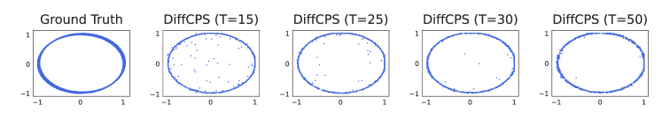
Before showing our method, we first present that the limited policy expressivity in previous Advantage Weighted Regression (AWR) methods (Peters et al., 2010; Peng et al., 2019; Nair et al., 2020) may degrade the performance through a sample 2-D bandit experiment with real-valued actions. Our offline dataset is constructed by a unit circle with noise (The first panel of Figure 1). Data on the noisy circle have a positive reward of $1$. Note that this offline dataset exhibits strong multi-modality since there are many actions (points on the noisy circle) that can achieve the same reward of $1$ if a state is given. However, if we use unimodal Gaussian to represent the policy, although the points on the noisy circle can all receive the same reward of $1$, the actions taken by AWR will move closer to the center of the noisy circle (AWR in Figure 1), due to the incorrect unimodal assumption. Experiment results in Figure 1 illustrate that AWR performs poorly in the bandit experiments compared to other diffusion-based methods. We also notice that compared to other diffusion-based methods, actions generated by SfBC include many points that differ significantly from those in the dataset, when $T=15$. This is due to the sampling error introduced by incorporating diffusion into AWR.

Therefore, we conclude that policy expressivity is important in offline RL since most offline RL datasets are collected from multiple behavior policies or human experts, which exhibit strong multi-modality. To better model behavior policies, we need more expressive generative models to model the policy distribution, rather than using unimodal Gaussians. Furthermore, we also need to avoid the sampling errors caused by using diffusion in AWR, which is the motivation behind our algorithm.

In this subsection, we focus on deriving our diffusion-based CPS problem Eq. (12). Firstly, we present the form of constrained policy search (Peng et al., 2019):

where $\mu({\bm{a}}|{\bm{s}})$ denotes our diffusion-based policy, $\pi_{b}$ denotes the behavior policy. Here we represent our policy $\mu({\bm{a}}|{\bm{s}})$ via the conditional diffusion model:

where the end sample of the reverse chain ${\bm{a}}^{0}$ is the action used for the policy’s output and $\mu({\bm{a}}^{0:T})$ is the joint distribution of all noisy samples. According to DDPM, we can approximate the reverse process $\mu({\bm{a}}^{i-1}|{\bm{a}}^{i},{\bm{s}})$ with a Gaussian distribution ${\mathcal{N}}({\bm{a}}^{i-1};{\bm{\mu}}_{\theta}({\bm{a}}^{i},{\bm{s}},i),{\bm{\Sigma}}_{\theta}({\bm{a}}^{i},{\bm{s}},i))$. We also follow the DDPM to fix the covariance matrix and predict the mean with a conditional noise model ${\mathbf{\epsilon}}_{\theta}({\bm{a}}^{i},{\bm{s}},i)$:

In the reverse process, we sample ${\bm{a}}^{T}\sim{\mathcal{N}}(\mathbf{0},{\bm{I}})$ and then follow the reverse diffusion chain ${\mathcal{N}}\left\{{\bm{a}}^{i-1}|{\bm{a}}^{i}\right\}$, parameterized by $\theta$ as

for $i=T,\ldots,1.$ The reverse sampling in Eq. (11) requires iteratively predicting ${\mathbf{\epsilon}}$ $T$ times. When $T$ is large, it will consume much time during the sampling process. To work with small $T$ ($T=5$ in our experiment), we follow (Xiao et al., 2021; Wang et al., 2022) and define

which is a noise schedule obtained under the variance preserving SDE of Song et al. (2020).

According to Theorem 3.7, we can get the optimal policy by solving the dual problem. In the following section, we outline the algorithm for solving Eq. (12). It consists of two steps: (i) solving the unconstrained dual function of Eq. (12), (ii) updating the Lagrange multiplier.

In this section, the duality is used to solve the Eq. (12) and derive our method. The dual function of Eq. (12) is

The Lagrange dual problem associated with the Eq. (12) is

In Eq. (14), we need to calculate the cross entropy $H(\pi_{b},\mu)$, which is intractable in practice.

In practice, to turn the original functional optimization problem into a tractable problem, we often use parametrized policies, such as neural networks. Next, we shift focus to solving the parametric version of Eq. (12), $i.e.$ to find the parametrized policies $\mu_{\theta}$ that solve Eq. (14)

Notice that we follow Fujimoto & Gu (2021); Wang et al. (2022) to normalize $Q^{\mu}({\bm{s}},{\bm{a}})$ by dividing it by the target Q-net’s value. We also clip the $\lambda$ to keep the constraint $\lambda\geq 0$ holding by $\lambda_{\text{clip}}=\max(c,\lambda)$, $c\geq 0$. We also find that we can improve the performance of the policy by delaying the policy update (Fujimoto et al., 2018). The algorithm given by Eq. (17)-Eq. (18) for solving Eq. (12) is summarized under Algorithm 1.

However, there is a cost for introducing such parametrization in Algorithm 1: the duality gap is no longer null. In the following Theorem 3.11, we show that after introducing parameterization, we can obtain a suboptimal solution in a ${\mathcal{O}}(1/\epsilon)$ number of dual iterations. Below, we first define $\epsilon$-universal parametrization functions.

Theoretically, we need to precisely solve the Eq. (17) and Eq. (18). However, in practice, we can resort to SGD and parametrized policy to solve the equations. In this way, we can recursively optimize Eq. (12) through Eq. (17) and Eq. (18). The policy improvement described in Eq. (17) and the solution of Eq. (18) constitute the core of DiffCPS.

In Table 1, we compare the performance of DiffCPS to other offline RL methods in D4RL (Fu et al., 2020) tasks. We merely illustrate the results of the MuJoCo locomotion and AntMaze tasks due to the page limit. In traditional MuJoCo tasks, DiffCPS outperforms other methods as well as recent diffusion-based method (Wang et al., 2022; Lu et al., 2023; Hansen-Estruch et al., 2023) by large margins in most tasks, especially in the HalfCheetah medium. The medium datasets are collected by online SAC (Haarnoja et al., 2018a) agent trained to approximate $1/3$ the performance of the expert. Hence, it contains a lot of suboptimal trajectories, which makes the offline RL algorithms hard to learn.

Compared to the locomotion tasks, AntMaze tasks are more challenging since the datasets consist of sparse rewards and suboptimal trajectories. Even so, DiffCPS also achieves competitive or SOTA results compared with other methods. For simpler tasks like umaze, DiffCPS achieves $100\pm 0\%$ success rate on some seeds, which shows its powerful ability to learn from suboptimal trajectories. In other AntMaze tasks, DiffCPS also shows competitive performance compared to other SOTA diffusion-based approaches. Overall, the experiments demonstrate the effectiveness of DiffCPS compared to several existing methods for offline RL.

In this section, we analyze why DiffCPS outperforms the other methods quantitatively on D4RL tasks. We conduct an ablation study to investigate the impact of three parts in DiffCPS, $i.e.$ diffusion steps, the minimum value of Lagrange multiplier $\lambda_{\text{clip}}$, and policy evaluation interval.

Diffusion Steps. We show the effect of diffusion steps $T$, which is a vital hyperparameter in all diffusion-based methods. In SfBC the best $T$ is $15$, while $T=5$ is best for our DiffCPS. Table 2 shows the average performance of different diffusion steps. Figure 2 shows the training curve of selected D4RL tasks over different diffusion steps $T$.

We also note that large $T$ works better for the bandit experiment. However, for D4RL tasks, a large $T$ will lead to a performance drop. The reason is that compared to bandit tasks, D4RL datasets contain a significant amount of suboptimal trajectories. A larger $T$ implies stronger behavior cloning ability, which can indeed lead to policy overfitting to the suboptimal data, especially when combined with actor-critic methods. Poor policies result in error value estimates, and vice versa, creating a vicious cycle that leads to a drop in policy performance with a large $T$.

The Minimum Value of Lagrange multiplier $\lambda_{\text{clip}}$. In our method, $\lambda$ serves as the coefficient for the policy constraint term, where a larger $\lambda$ implies a stronger policy constraint. Although we need to restrict the $\lambda\geq 0$ according to the definition of Lagrange multiplier, we notice that we could get better results through clip $\lambda\geq c$ in AntMaze tasks, where $c$ is a positive number, see full $\lambda$ ablation results in Figure 3 for details.

Policy Evaluation Interval. We include the ablation of policy evaluation interval in Figure 4. We find that the policy delayed update (Fujimoto et al., 2018) has significant impacts on AntMaze large tasks. However, for other tasks, it does not have much effect and even leads to a slight performance decline. The reason is that infrequent policy updates reduce the variance of value estimates, which is more effective in tasks where sparse rewards and suboptimal trajectories lead to significant errors in value function estimation like AntMaze large tasks.

In a nutshell, the ablation study shows that the combination of these three parts, along with DiffCPS, collectively leads to producing good performance.

References

- Ajay et al. (2022) Ajay, A., Du, Y., Gupta, A., Tenenbaum, J. B., Jaakkola, T. S., and Agrawal, P. Is conditional generative modeling all you need for decision making? In The Eleventh International Conference on Learning Representations, 2022.
- Borkar (1988) Borkar, V. S. A convex analytic approach to markov decision processes. Probability Theory and Related Fields, 78(4):583–602, 1988.
- Boyd & Vandenberghe (2004) Boyd, S. P. and Vandenberghe, L. Convex optimization. Cambridge university press, 2004.
- (4) Chen, H., Lu, C., Wang, Z., Su, H., and Zhu, J. Score regularized policy optimization through diffusion behavior. URL http://arxiv.org/abs/2310.07297.
- Chen et al. (2022) Chen, H., Lu, C., Ying, C., Su, H., and Zhu, J. Offline reinforcement learning via high-fidelity generative behavior modeling. In The Eleventh International Conference on Learning Representations, 2022.
- Chen et al. (2021) Chen, L., Lu, K., Rajeswaran, A., Lee, K., Grover, A., Laskin, M., Abbeel, P., Srinivas, A., and Mordatch, I. Decision transformer: Reinforcement learning via sequence modeling. Advances in neural information processing systems, 34:15084–15097, 2021.
- Chen et al. (2020) Chen, X., Zhou, Z., Wang, Z., Wang, C., Wu, Y., and Ross, K. Bail: Best-action imitation learning for batch deep reinforcement learning. Advances in Neural Information Processing Systems, 33:18353–18363, 2020.
- Dhariwal & Nichol (2021) Dhariwal, P. and Nichol, A. Diffusion models beat gans on image synthesis. Advances in neural information processing systems, 34:8780–8794, 2021.
- Fu et al. (2020) Fu, J., Kumar, A., Nachum, O., Tucker, G., and Levine, S. D4rl: Datasets for deep data-driven reinforcement learning. arXiv preprint arXiv:2004.07219, 2020.
- Fujimoto & Gu (2021) Fujimoto, S. and Gu, S. S. A minimalist approach to offline reinforcement learning. Advances in neural information processing systems, 34:20132–20145, 2021.
- Fujimoto et al. (2018) Fujimoto, S., Hoof, H., and Meger, D. Addressing function approximation error in actor-critic methods. In International Conference on Machine Learning, pp. 1587–1596. PMLR, 2018.
- Fujimoto et al. (2019) Fujimoto, S., Meger, D., and Precup, D. Off-policy deep reinforcement learning without exploration. In International Conference on Machine Learning, pp. 2052–2062. PMLR, 2019.
- Ghasemipour et al. (2020) Ghasemipour, S. K. S., Schuurmans, D., and Gu, S. S. Emaq: Expected-max q-learning operator for simple yet effective offline and online rl. arXiv preprint arXiv:2007.11091, 2020.
- (14) Gürtler, N., Blaes, S., Kolev, P., Widmaier, F., Wüthrich, M., Bauer, S., Schölkopf, B., and Martius, G. BENCHMARKING OFFLINE REINFORCEMENT LEARN- ING ON REAL-ROBOT HARDWARE.
- Haarnoja et al. (2018a) Haarnoja, T., Zhou, A., Abbeel, P., and Levine, S. Soft actor-critic: Off-policy maximum entropy deep reinforcement learning with a stochastic actor. In International Conference on Machine Learning, pp. 1861–1870. PMLR, 2018a.
- Haarnoja et al. (2018b) Haarnoja, T., Zhou, A., Hartikainen, K., Tucker, G., Ha, S., Tan, J., Kumar, V., Zhu, H., Gupta, A., and Abbeel, P. Soft actor-critic algorithms and applications. arXiv preprint arXiv:1812.05905, 2018b.
- Hansen-Estruch et al. (2023) Hansen-Estruch, P., Kostrikov, I., Janner, M., Kuba, J. G., and Levine, S. Idql: Implicit q-learning as an actor-critic method with diffusion policies. arXiv preprint arXiv:2304.10573, 2023.
- Ho & Salimans (2021) Ho, J. and Salimans, T. Classifier-free diffusion guidance. In NeurIPS 2021 Workshop on Deep Generative Models and Downstream Applications, 2021.
- Ho et al. (2020) Ho, J., Jain, A., and Abbeel, P. Denoising diffusion probabilistic models. Advances in neural information processing systems, 33:6840–6851, 2020.
- Janner et al. (2022) Janner, M., Du, Y., Tenenbaum, J. B., and Levine, S. Planning with diffusion for flexible behavior synthesis. arXiv preprint arXiv:2205.09991, 2022.
- (21) Kang, B. and Ma, X. Efficient diffusion policies for offline reinforcement learning.
- Kidambi et al. (2020) Kidambi, R., Rajeswaran, A., Netrapalli, P., and Joachims, T. Morel: Model-based offline reinforcement learning. Advances in neural information processing systems, 33:21810–21823, 2020.
- Kingma & Ba (2014) Kingma, D. P. and Ba, J. Adam: A method for stochastic optimization. arXiv preprint arXiv:1412.6980, 2014.
- Kingma & Welling (2013) Kingma, D. P. and Welling, M. Auto-encoding variational bayes. arXiv e-prints, pp. arXiv–1312, 2013.
- Kostrikov et al. (2021a) Kostrikov, I., Fergus, R., Tompson, J., and Nachum, O. Offline reinforcement learning with fisher divergence critic regularization. In International Conference on Machine Learning, pp. 5774–5783. PMLR, 2021a.
- Kostrikov et al. (2021b) Kostrikov, I., Nair, A., and Levine, S. Offline reinforcement learning with implicit q-learning. In International Conference on Learning Representations, 2021b.
- Kumar et al. (2019) Kumar, A., Fu, J., Soh, M., Tucker, G., and Levine, S. Stabilizing off-policy q-learning via bootstrapping error reduction. Advances in Neural Information Processing Systems, 32, 2019.
- Kumar et al. (2020) Kumar, A., Zhou, A., Tucker, G., and Levine, S. Conservative q-learning for offline reinforcement learning. Advances in Neural Information Processing Systems, 33:1179–1191, 2020.
- Levine et al. (2020) Levine, S., Kumar, A., Tucker, G., and Fu, J. Offline reinforcement learning: Tutorial, review, and perspectives on open problems. arXiv preprint arXiv:2005.01643, 2020.
- Liang et al. (2023) Liang, Z., Mu, Y., Ding, M., Ni, F., Tomizuka, M., and Luo, P. Adaptdiffuser: Diffusion models as adaptive self-evolving planners. arXiv preprint arXiv:2302.01877, 2023.
- Lillicrap et al. (2015) Lillicrap, T. P., Hunt, J. J., Pritzel, A., Heess, N., Erez, T., Tassa, Y., Silver, D., and Wierstra, D. Continuous control with deep reinforcement learning. arXiv preprint arXiv:1509.02971, 2015.
- Lu et al. (2023) Lu, C., Chen, H., Chen, J., Su, H., Li, C., and Zhu, J. Contrastive energy prediction for exact energy-guided diffusion sampling in offline reinforcement learning. arXiv preprint arXiv:2304.12824, 2023.
- Ma et al. (2021) Ma, X., Yang, Y., Hu, H., Liu, Q., Yang, J., Zhang, C., Zhao, Q., and Liang, B. Offline reinforcement learning with value-based episodic memory. arXiv preprint arXiv:2110.09796, 2021.
- (34) Matsushima, T., Furuta, H., Matsuo, Y., Nachum, O., and Gu, S. S. Deployment-efficient reinforcement learn-ing via model-based offline optimization. Policy, 100:1000s.
- Nair et al. (2020) Nair, A., Gupta, A., Dalal, M., and Levine, S. Awac: Accelerating online reinforcement learning with offline datasets. arXiv preprint arXiv:2006.09359, 2020.
- Nie et al. (2021) Nie, X., Brunskill, E., and Wager, S. Learning when-to-treat policies. Journal of the American Statistical Association, 116(533):392–409, 2021.
- Paternain et al. (2019) Paternain, S., Chamon, L., Calvo-Fullana, M., and Ribeiro, A. Constrained reinforcement learning has zero duality gap. Advances in Neural Information Processing Systems, 32, 2019.
- Pearce et al. (2023) Pearce, T., Rashid, T., Kanervisto, A., Bignell, D., Sun, M., Georgescu, R., Macua, S. V., Tan, S. Z., Momennejad, I., Hofmann, K., et al. Imitating human behaviour with diffusion models. arXiv preprint arXiv:2301.10677, 2023.
- Peng et al. (2019) Peng, X. B., Kumar, A., Zhang, G., and Levine, S. Advantage-weighted regression: Simple and scalable off-policy reinforcement learning. arXiv preprint arXiv:1910.00177, 2019.
- Peters et al. (2010) Peters, J., Mulling, K., and Altun, Y. Relative entropy policy search. In Proceedings of the AAAI Conference on Artificial Intelligence, volume 24, pp. 1607–1612, 2010.
- Rashidinejad et al. (2021) Rashidinejad, P., Zhu, B., Ma, C., Jiao, J., and Russell, S. Bridging offline reinforcement learning and imitation learning: A tale of pessimism. Advances in Neural Information Processing Systems, 34:11702–11716, 2021.
- Rhinehart et al. (2018) Rhinehart, N., McAllister, R., and Levine, S. Deep imitative models for flexible inference, planning, and control. arXiv preprint arXiv:1810.06544, 2018.
- Rockafellar (1970) Rockafellar, R. Convex analysis. Princeton Math. Series, 28, 1970.
- Shafiullah et al. (2022) Shafiullah, N. M., Cui, Z., Altanzaya, A. A., and Pinto, L. Behavior transformers: Cloning modes with one stone. Advances in neural information processing systems, 35:22955–22968, 2022.
- Sohl-Dickstein et al. (2015) Sohl-Dickstein, J., Weiss, E., Maheswaranathan, N., and Ganguli, S. Deep unsupervised learning using nonequilibrium thermodynamics. In International Conference on Machine Learning, pp. 2256–2265. PMLR, 2015.
- Song & Ermon (2019) Song, Y. and Ermon, S. Generative modeling by estimating gradients of the data distribution. Advances in neural information processing systems, 32, 2019.
- Song et al. (2020) Song, Y., Sohl-Dickstein, J., Kingma, D. P., Kumar, A., Ermon, S., and Poole, B. Score-based generative modeling through stochastic differential equations. arXiv preprint arXiv:2011.13456, 2020.
- Suh et al. (2023) Suh, H., Chou, G., Dai, H., Yang, L., Gupta, A., and Tedrake, R. Fighting uncertainty with gradients: Offline reinforcement learning via diffusion score matching. arXiv preprint arXiv:2306.14079, 2023.
- Sutton & Barto (2018) Sutton, R. S. and Barto, A. G. Reinforcement Learning: An Introduction. MIT press, 2018.
- Tseng et al. (2017) Tseng, H.-H., Luo, Y., Cui, S., Chien, J.-T., Ten Haken, R. K., and Naqa, I. E. Deep reinforcement learning for automated radiation adaptation in lung cancer. Medical physics, 44(12):6690–6705, 2017.
- Wang et al. (2020) Wang, Z., Novikov, A., Zolna, K., Merel, J. S., Springenberg, J. T., Reed, S. E., Shahriari, B., Siegel, N., Gulcehre, C., and Heess, N. Critic regularized regression. Advances in Neural Information Processing Systems, 33:7768–7778, 2020.
- Wang et al. (2022) Wang, Z., Hunt, J. J., and Zhou, M. Diffusion policies as an expressive policy class for offline reinforcement learning. arXiv preprint arXiv:2208.06193, 2022.
- Wu et al. (2019) Wu, Y., Tucker, G., and Nachum, O. Behavior regularized offline reinforcement learning. arXiv preprint arXiv:1911.11361, 2019.
- Xiao et al. (2021) Xiao, Z., Kreis, K., and Vahdat, A. Tackling the generative learning trilemma with denoising diffusion gans. arXiv preprint arXiv:2112.07804, 2021.
- Yu et al. (2020) Yu, T., Thomas, G., Yu, L., Ermon, S., Zou, J. Y., Levine, S., Finn, C., and Ma, T. Mopo: Model-based offline policy optimization. Advances in Neural Information Processing Systems, 33:14129–14142, 2020.
- Yurtsever et al. (2020) Yurtsever, E., Lambert, J., Carballo, A., and Takeda, K. A survey of autonomous driving: Common practices and emerging technologies. IEEE access, 8:58443–58469, 2020.
In the appendix, we provide the proofs of the main theorems in the paper (Appendix A), the notation table (Appendix B), details of the experiments (Appendix C), some additional experiments (Appendix D,F,E), and a discussion on the use of the augmented Lagrangian method (Appendix G).
Appendix A Proofs
A.1 Theorem 3.1
We provide the proof of Theorem 3.1.
Proof.
(1): Since the pointwise KL constraint in Eq. (2.1) at all states is intractable, we follow the Peng et al. (2019) to relax the constraint by enforcing it only in expectation
The LHS can be transformed to