Diamonds are Forever in the Blockchain:
Geometric Polyhedral Point-Set Pattern Matching

Gill Barequet Dept. of Computer Science, Technion—Israel Inst. of Technology, [email protected] Shion Fukuzawa Dept. of Computer Science, University of California, Irvine, {fukuzaws,goodrich,mosegued,eozel}@uci.edu Michael T. Goodrich^† David M. Mount Dept. of Computer Science, University of Maryland, College Park, [email protected] Martha C. Osegueda^† Evrim Ozel^†

Abstract

Motivated by blockchain technology for supply-chain tracing of ethically sourced diamonds, we study geometric polyhedral point-set pattern matching as minimum-width polyhedral annulus problems under translations and rotations. We provide two $(1+\varepsilon)$ -approximation schemes under translations with $O(\varepsilon^{-d}n)$ -time for $d$ dimensions and $O(n\log\varepsilon^{-1}+\varepsilon^{-2})$ -time for two dimensions, and we give an $O(f^{d-1}\varepsilon^{1-2d}n)$ -time algorithm when also allowing for rotations, parameterized on $f$ , which we define as the slimness of the point set.

1 Introduction

A notable recent computational geometry application is for tracking supply chains for natural diamonds, for which the industry and customers are strongly motivated to prefer ethically-sourced provenance (e.g., to avoid so-called “blood diamonds”). For example, the Tracr system employs a blockchain for tracing the supply chain for a diamond from its being mined as a rough diamond to a customer purchasing a polished diamond [23]. (See Figure 1.)

Refer to caption — Figure 1: Blockchain transactions in a diamond supply chain, providing provenance, traceability, and authenticity of an ethically-sourced diamond.

Essential steps in the Tracr blockchain supply-chain process require methods to match point sets against geometric shapes, e.g., to guarantee that a diamond has not been replaced with one of questionable provenance [23]. Currently, the Tracr system uses standard machine-learning techniques to perform the shape matching steps. We believe, however, that better accuracy can be achieved by using computational geometry approaches. In particular, motivated by the Tracr application, we are interested in this paper in efficient methods for matching point sets against geometric shapes, such as polyhedra. Formalizing this problem, we study the problem of finding the best translation and/or rotation of the boundary of a convex polytope, $P$ (e.g., defining a polished diamond shape), to match a set of $n$ points in a $d$ -dimensional ( $d\geq 3$ ) space, where the point set is a “good” sample of the boundary of a polytope that is purported to be $P$ . Since there may be small inaccuracies in the sampling process, our aim is to compute a minimum width polyhedral annulus determined by $P$ that contains the sampled points. In the interest of optimizing running time, rather than seeking an exact solution, we seek an approximate solution that deviates from the real solution by a predefined quantity $\varepsilon>0$ .

Related Work.

We are not familiar with any previous work on the problems we study in this paper. Nevertheless, there is considerable prior work on the general area of matching a geometric shape to a set of points, especially in the plane. For example, Barequet, Bose, Dickerson, and Goodrich [12] give solutions to several constrained polygon annulus placement problems for offset and scaled polygons including an algorithm for finding the translation for the minimum offset of an $m$ -vertex polygon that contains a set of $n$ points in $O(n\log^{2}n+m)$ time. Barequet, Dickerson, and Scharf [13] study the problem of covering a maximum number of $n$ points with an $m$ -vertex polygon (not just its boundary) under translations, rotations, and/or scaling, giving, e.g., an algorithm running in time $O(n^{3}m^{4}\log(nm))$ for the general problem. There has also been work on finding a minimum-width annulus for rectangles and squares, e.g., see [19, 9, 11, 21].

Chan [15] presents a $(1+\varepsilon)$ -approximation method that finds a minimum-width spherical annulus of $n$ points in $d$ dimensions in $O(n\log(1/\varepsilon)+\varepsilon^{O(1)})$ time, and Agarwal, Har-Peled, and Varadarajan [1] improve this to $O(n+1/\varepsilon^{O(d^{2})})$ time via coresets [2, 22, 24, 3]. A line of work has considered computing the spherical annulus under stronger assumptions on the points samples. Most notably Devillers and Ramos [17] combine various definitions for “minimum quality assumptions” by Melhorn, Shermer and Yap [20] and Bose and Morin [14] and show that under this assumption the spherical annulus can be computed in linear time for $d=2$ and present empirical evidence for higher dimensions. Arya, da Fonseca, and Mount [6] show how to find an $\varepsilon$ -approximation of the width of $n$ points in $O(n\log(1/\varepsilon)+1/\varepsilon^{(d-1)/2+\alpha})$ time, for a constant $\alpha>0$ . Bae [10] shows how to find a min-width $d$ -dimensional hypercubic shell in $O(n^{\lfloor d/2\rfloor}\log^{d-1}n)$ expected time.

Our Results.

Given a set of $n$ points in ${\bf R}^{d}$ , we provide an $O(\varepsilon^{-d}n)$ -time $(1+\varepsilon)$ -approximate polytope-matching algorithm under translations, for $d\geq 3$ , and $O(n\log\varepsilon^{-1}+\varepsilon^{-2})$ time for $d=2$ , and we provide an $O(f^{d-1}\varepsilon^{1-2d}n)$ -time algorithm when also allowing for rotations, where the complexity of the polytope is constant and for rotations is parameterized by $f$ , which we define as the slimness of the point set.

The paper is organized as follows. In Section 2, we set the ground for this work by providing some necessary definitions. In Section 3, we approximate the MWA under only translations. In this section, we provide a constant factor approximation scheme, a $(1+\varepsilon)$ -approximation scheme and describe how to improve the running time in two dimensions. In Section 4, we consider the MWA under rotations.

2 Preliminaries

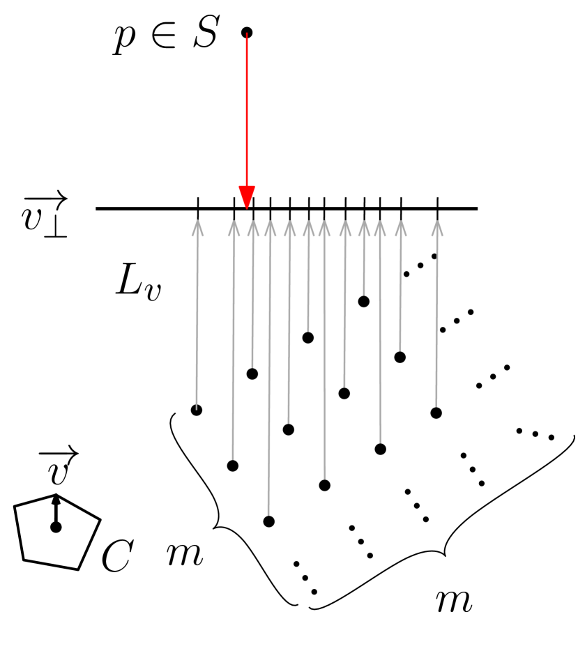
Following previous convention [4, 7, 8, 18, 5], we say that a point set $S$ is a $\delta$ -uniform sample of a surface $\Sigma\subset\mathbb{R}^{d}$ if for every point $p\in\Sigma$ , there exists a point $q\in S$ such that $d(p,q)\leq\delta$ . Let $C\subset\mathbb{R}^{d}$ be a closed, convex polyhedron containing the origin in its interior. Given $C$ , and $x\in\mathbb{R}^{d}$ , define $x+C=\{x+y:y\in C\}$ (the translation of $C$ by $x$ ), and for $r\in\mathbb{R}$ , define $rC=\{ry:y\in C\}$ . A placement of $C$ is a pair $(x,r)$ , where $x\in\mathbb{R}^{d}$ and $r\in\mathbb{R}^{\geq 0}$ , representing the translated and scaled copy $x+rC$ . We refer to $x$ and $r$ as the center and radius of the placement, respectively. Two placements are concentric if they share the same center.

Let $C$ be any closed convex body in $\mathbb{R}^{d}$ containing the origin in its interior. The convex distance function induced by $C$ is the function $d_{C}:\mathbb{R}^{d}\times\mathbb{R}^{d}\rightarrow\mathbb{R}^{\geq 0}$ , where

d_{C}(p,q)=\min\{r:r\geq 0~{}\mathrm{and}~{}q\in p+rC\}

Thus, the convex distance between $p$ and $q$ is determined by the minimum radius placement of $C$ centered at $p$ that contains $q$ (see Figure 2). When $C$ is centrally symmetric, this defines a metric, but for general $C$ , the function $d_{C}$ may not be symmetric. We call the original shape $C$ the unit ball $U_{C}$ under the distance function $d_{C}$ . Note that $d_{C}(a,c)=d_{C}(a,b)+d_{C}(b,c)$ when $a$ , $b$ and $c$ are collinear and appear in that order.

Define an annulus for $C$ to be the set-theoretic difference of two concentric placements $(p+RC)\setminus(p+rC)$ , for $0\leq r\leq R$ . The width of the annulus is $R-r$ . Given a $\delta$ -uniform sample of points, $S$ , there are three placements of $C$ we are interested in:

$\bullet$ Minimum enclosing ball (MinBall): A placement of $C$ of the smallest radius that contains all of the points in $S$ .

$\bullet$ Maximum enclosed ball (MaxBall): A placement of $C$ of the largest radius, centered within the convex hull of $S$ , that contains no points in $S$ .

$\bullet$ Minimum width annulus (MWA): A placement of an annulus for $C$ of minimum width, that contains all of the points in $S$ .

Note that, following the definition of the MaxBall, we require that the center of the MWA must also lie within the convex hull of $S$ . For each of the above placements, we also refer to parameterized versions, for example MinBall( $p$ ), MaxBall( $p$ ), or MWA( $p$ ). These respectively refer to the minimum enclosing ball, maximum enclosed ball, or minimum width annulus centered at the point $p$ .

Further, we use $|{\rm MinBall}(p)|$ and $|{\rm MaxBall}(p)|$ to denote the radius of MinBall $(p)$ and MaxBall $(p)$ , respectively, and we use $|{\rm MWA}(p)|$ to denote the width of MWA $(p)$ .

The ratio, $F$ , of the MinBall over the MaxBall of $S\subset\mathbb{R}^{d}$ under distance function $d_{C}$ defines the fatness of $S$ under $d_{C}$ , such that $F:=|{\rm MinBall}|/|{\rm MaxBall}|$ . Also, we define the concentric fatness as the ratio of the MinBall and MaxBall centered at the MWA, such that $F_{c}:=|{\rm MinBall}(c_{opt})|/|{\rm MaxBall}(c_{opt})|$ where $c_{opt}$ is the center of the MWA. Conversely, we define the slimness to be $f^{-1}=1-F_{c}^{-1}$ , which corresponds to the ratio of the ${\rm MinBall}(c_{opt})$ over the MWA, i.e., $f:=|{\rm MinBall}(c_{opt})|/|{\rm MWA}|$ .

Remark 1

In order for a $\delta$ -uniform sample to represent the surface, $\Sigma$ , with sufficient accuracy for a meaningful ${\rm MWA}$ , we assume that the sample must contain at least one point between corresponding facets of the ${\rm MWA}$ . Where corresponding facets refer to facets of the ${\rm MinBall}$ and ${\rm MaxBall}$ representing the same facet of $U_{C}$ . Therefore, in the remainder of the paper, we assume we have a $\delta$ -uniform sample and that $\delta$ is small enough to guarantee this condition for even the smallest facets.

In practice, it would be easy to determine a small enough $\delta$ before sampling $\Sigma$ , since only sufficiently slim surfaces would benefit from finding the ${\rm MWA}$ , and very fat surfaces would yield increasingly noisy ${\rm MaxBall}$ . One easy approach would be setting $\delta$ to the smallest facet of the ${\rm MinBall}$ and scaling down by an arbitrary constant larger than the maximum expected fatness, such as 100. This example imposes a very generous bound on fatness since it would allow the inner shell to be 1% of the size of the outer shell, practically a single digit constant would often suffice.

Also, note that, for a given center point $c$ , ${\rm MWA}(c)$ is uniquely defined as the annulus centered at $c$ with inner radius $\min_{p\in S}d_{C}(c,p)$ and outer radius $\max_{p\in S}d_{C}(c,p)$ . Further, let us assume that the reference polytope defining our polyhedral distance function has $m$ facets, where $m$ is a fixed constant, since the sample size is expected to be much larger than $m$ . Thus, $d_{C}$ can be calculated in $O(m)$ time; hence, ${\rm MWA}(c)$ can be found in $O(mn)$ time, which is $O(n)$ under our assumption.

3 Approximating the Minimum Width Annulus

Let us first describe how to find a constant factor approximation of ${\rm MWA}$ under translations. Note that, by assumption, the center $c$ of our approximation lies within the convex hull of $S$ . Let us denote the center, outer radius, inner radius, and width of the optimal MWA as $c_{opt}$ , $R_{opt}$ , $r_{opt}$ , and $w_{opt}$ .

We begin with Lemma 3.1, where we prove $c_{opt}$ is within a certain distance from the center of the MinBall $c$ , providing a search region for $c_{opt}$ . In Lemma 3.3, we bound the width achieved by a center-point that is sufficiently close to $c_{opt}$ . We then use this in Lemma 3.5 to prove that $|{\rm MWA}(c)|$ achieves a constant factor approximation.

Lemma 3.1.

The center of the ${\rm MWA}$ , $c_{opt}$ , is within distance $w_{opt}$ of the center of the ${\rm MinBall}$ , $c$ . That is, $d_{C}(c,c_{opt})\leq w_{opt}$ .

Proof 3.2.

Recall our assumption from Remark 1. By our assumption that at least one sample point lies on each facet, MinBall cannot shrink past any facets of MaxBall( $c_{opt}$ ).

Suppose for contradiction that $d_{C}(c,c_{opt})>w_{opt}$ . Let $s$ be the point where a ray projected from $c$ through $c_{opt}$ intersects the boundary of MaxBall( $c_{opt}$ ), and let $R$ denote the radius of the MinBall. Observe that $R$ must be large enough for MinBall to contain $s$ and therefore $R\geq d_{C}(c,s)$ .

$\displaystyle R$	$\displaystyle\geq d_{C}(c,c_{opt})+d_{C}(c_{opt},s)$	by collinearity
	$\displaystyle>w_{opt}+d_{C}(c_{opt},s)$	by assumption
	$\displaystyle=w_{opt}+r_{opt}$	by MaxBall( $c_{opt}$ ).

Thus, since $w_{opt}+r_{opt}=R_{opt}$ , we find $R>R_{opt}$ , which is a contradiction since $R$ must be the smallest radius of the MinBall across all possible centers. Therefore, we have that $d_{C}(c,c_{opt})$ cannot be larger than $w_{opt}$ .

Lemma 3.1 helps us constrain the region within which $c$ must be contained. Let us now reason about how a given center point, $c$ , would serve as an approximation. For convenience, let us define $R:=|{\rm MinBall}(c)|$ and $r:=|{\rm MaxBall}(c)|$ as the radii of the MinBall and MaxBall centered at $c$ , respectively.

Lemma 3.3.

Suppose $c$ is an arbitrary center-point in our search region, and the two directed distances between $c$ and $c_{opt}$ are at most $t$ , i.e., $t\geq\max\{d_{C}(c,c_{opt}),d_{C}(c_{opt},c)\}$ . Then, we have that $|{\rm MWA}(c)|\leq w_{opt}+2t$ .

Proof 3.4.

Knowing that all sample points must be contained within the ${\rm MWA}$ , the ${\rm MWA}(c)$ cannot expand past the furthest or closest point in ${\rm MWA}$ from $c$ under $d_{C}$ . Let us now define these two points and use them to bound the radii for ${\rm MinBall}(c)$ and ${\rm MaxBall}(c)$ .

Let $p$ be the point where the ray from $c$ through $c_{opt}$ intersects the boundary of MinBall( $c_{opt}$ ). ${\rm MinBall}(c)$ cannot extend further than $p$ .

	$\displaystyle d_{C}(c,p)=d_{C}(c,c_{opt})+d_{C}(c_{opt},p)$	$\displaystyle\leq t+d_{C}(c_{opt},p)$
	$\displaystyle R$	$\displaystyle\leq R_{opt}+t.$

Conversely, let $q$ be the intersection point where the ray projected from $c_{opt}$ through $c$ intersects the boundary of MaxBall( $c_{opt}$ ), in which case ${\rm MaxBall}(c)$ cannot collapse further than $q$ .

	$\displaystyle d_{C}(c,q)=d_{C}(c_{opt},q)-d_{C}(c_{opt},c)$	$\displaystyle\geq d_{C}(c_{opt},q)-t$
	$\displaystyle r$	$\displaystyle\geq r_{opt}-t.$

Combining these bounds with the fact that $|MWA(c)|=R-r$ we find that $|\text{MWA}(c)|\leq w_{opt}+2t$ .

For simplicity, let us consider two points $a,b$ to be $t$ -close (under $C$ ) whenever $t\geq\max\{d_{C}(a,b),d_{C}(b,a)\}$ .

Lemma 3.5.

If $c$ is the center of ${\rm MinBall}$ , then ${\rm MWA}(c)$ is a constant factor approximation of the ${\rm MWA}$ , that is, $|{\rm MWA}(c)|\leq b|{\rm MWA}|$ , for some constant $b\geq 1$ , under translations.

Proof 3.6.

From Lemma 3.1, we have that $d_{C}(c,c_{opt})\leq w_{opt}$ . If $c$ and $c_{opt}$ are $w_{opt}$ -close, then we can directly apply the second part of Lemma 3.3 to find $r\geq r_{opt}-w_{opt}$ and $R\leq R_{opt}$ , such that $|{\rm MWA}(c)|\leq R_{opt}-(r_{opt}-w_{opt})$ , thus proving that this is a 2-approximation. If $d_{C}$ is a metric, then $d_{C}(c_{opt},c)=d_{C}(c,c_{opt})$ and this must always be the case. However, if $d_{C}(c_{opt},c)>w_{opt}$ , then we must use the Euclidean distance to find $d_{C}(c_{opt},c)$ . Let vector $u:=c-c_{opt}$ , and let us define unit vectors with respect to $d_{C}$ and $d_{\overline{C}}$ , such that

	$\displaystyle\widehat{u}_{C}=\frac{u}{d_{C}(c_{opt},c)},\hskip 14.22636pt\widehat{u}_{\overline{C}}=\frac{\overline{u}}{d_{C}(c,c_{opt})}$
	$\displaystyle\|\|\widehat{u}_{C}\|\|\kern 1.0ptd_{C}(c_{opt},c)~{}=~{}\|\|u\|\|~{}=~{}\|\|\widehat{u}_{\overline{C}}\|\|\kern 1.0ptd_{C}(c,c_{opt})$
	$\displaystyle d_{C}(c_{opt},c)\leq\frac{\|\|\widehat{u}_{\overline{C}}\|\|}{\|\|\widehat{u}_{C}\|\|}w_{opt}$		from Lemma 3.1.

Under any convex distance function, $\frac{||\widehat{u}_{\overline{C}}||}{||\widehat{u}_{C}||}$ is bounded from above by $A=\max_{v\in\mathbb{R}^{d}}\frac{||\widehat{v}_{\overline{C}}||}{||\widehat{v}_{C}||}$ , which corresponds to finding the direction, $v$ , of the largest asymmetry in $U_{C}$ . Thus, by Lemma 3.3, $|{\rm MWA}(c)|\leq(A+1)w_{opt}$ . Under our (fixed) polyhedral distance function, $A$ is constant; hence, MWA( $c$ ) is a constant-factor approximation.

$(1+\varepsilon)$ -approximation.

Let us now describe how to compute a $(1+\varepsilon)$ -approximation of ${\rm MWA}$ .

We begin with Lemma 3.7, which defines how close to $c_{opt}$ is sufficient for a $(1+\varepsilon)$ -approximation. In Theorem 3.9, we define a grid of candidate center-points so that any point in the search region has a gridpoint sufficiently close to it.

Lemma 3.7.

Suppose $c_{opt}$ and $c$ are $({\varepsilon w}/(2b))$ -close, where $w=|{\rm MWA}(c_{M})|$ , $c_{M}$ is the center of ${\rm MinBall}$ , and $b$ is the constant from Lemma 3.5. Then, ${\rm MWA}(c)$ is a $(1+\varepsilon)$ -approximation of ${\rm MWA}$ under translations.

Proof 3.8.

It suffices to show that the width of our approximation only exceeds the optimal width by a factor of at most $(1+\varepsilon)$ .

Assuming $c$ and $c_{opt}$ are $t$ -close, and using Lemma 3.3, we require that $w_{opt}+2t\leq(1+\varepsilon)w_{opt}$ , i.e., $t\leq\varepsilon w_{opt}/2$ .

Let us then choose $t\leq{\varepsilon w}/(2b)$ , knowing that $w\leq bw_{opt}$ from Lemma 3.5, which is sufficient for achieving a $(1+\varepsilon)$ -approximation.

Knowing how close our approximation’s center must be, we can now present a $(1+\varepsilon)$ -approximation algorithm to find a center satisfying this condition.

Theorem 3.9.

One can achieve a $(1+\varepsilon)$ -approximation of the ${\rm MWA}$ under translations in $O(\varepsilon^{-d}n)$ time.

Proof 3.10.

The MinBall can be computed in $O(n)$ time [16]. By Lemma 3.1, we have that $d_{C}(c,c_{opt})\leq w_{opt}$ , where $c$ is the MinBall center. This implies that $c_{opt}$ must lie within the placement $c+w_{opt}C$ or more generously in $P$ , defined as $c+wC$ . Furthermore, from Lemma 3.7, we know that being $({\varepsilon w}/(2b))$ -close to $c_{opt}$ suffices for an $(1+\varepsilon)$ -approximation. Therefore, overlaying a grid $G$ that covers $P$ , such that any point in $p\in P$ is $({\varepsilon w}/(2b))$ -close to a gridpoint, guarantees the existence of a point $g\in G$ for which ${\rm MWA}(g)$ is a $(1+\varepsilon)$ -approximation.

Since $P$ and $({\varepsilon w}/(2b))$ -closeness are both defined under $d_{C}$ , we translate this to a cubic grid for simplicity. Let $Q$ be the smallest cube enclosing $P$ and $q$ be the largest cube enclosed by $({\varepsilon w}/(2b))C$ . Let us now define a grid, $G$ , to span over $Q$ with cells the size of $q$ .

This grid, $G$ , has $O(Fb/\varepsilon)$ gridpoints per direction and $O(F^{d}b^{d}\varepsilon^{-d})$ gridpoints in total, where $F$ corresponds to the fatness of $C$ under the cubic distance function.

Let us define the cubic distance function, $d_{q}$ , with unit cube $U_{q}=q\cdot(2b)/(\varepsilon w)$ , such that $U_{q}$ is the largest cube enclosed by $C$ .

The grid $G$ guarantees that for every point $p$ , there exists a gridpoint $g\in G$ such that $d_{q}(p,g)\leq{\varepsilon w}/(2b)$ . Since the unit cube is contained within the unit polyhedron, we have that $d_{C}(a,b)\leq d_{q}(a,b)\ \forall a,b$ ; and since $d_{q}$ defines a metric, $p$ must also be $({\varepsilon w}/(2b))$ -close under $d_{C}$ . Finding the gridpoint providing the $(1+\varepsilon)$ -approximation takes $O(F^{d}b^{d}\varepsilon^{-d}n)$ time,¹¹1For metrics, MinBall provides a 2-approximation, thus $b{=}2$ . For non-metrics, we can remove this constant by first using this algorithm with $\varepsilon{=}1$ in order to find a 2-approximation in linear-time, and using this approximation for gridding in the main step. which, under a fixed $d_{C}$ , is $O(\varepsilon^{-d}n)$ time.

Faster grid-search in two dimensions.

The algorithm of Theorem 3.9 recalculates the MWA at every gridpoint. However, small movements along the grid should not affect the MWA much. We use this insight to speed up MWA recalculations for two dimensions.

Let us first define the contributing edge of a sample point, $p\in S$ , as the edge of $C+g$ intersected by the ray emanating from a gridpoint, $g$ , towards $p$ . Under this center-point, $p$ will only directly affect the placement of the contributing edge. Observe that given vectors $\overrightarrow{v}\in C$ , defined as the vectors directed from the center towards each vertex, the planar subdivision, created by rays for each $\overrightarrow{v}$ originating from $g$ , separates points by their contributing edge. For any two gridpoints, $g_{1}$ and $g_{2}$ , and rays projected from them parallel to $\overrightarrow{v}$ , any points within these two rays will contribute to different edges under $g_{1}$ and $g_{2}$ . We denote this region as the vertex slab of vertex $v$ , and the regions outside of this as edge slabs. Points within an edge slab contribute to the same edge under both gridpoints, maintaining the constraints this imposes on the MWA, can therefore be achieved with the two extreme points per edge slab. If we consider vertex slabs for all $g\in G$ , we must be able to quickly calculate the strictest constraints imposed by points in a subset of vertex slabs. An example of the planar subdivision for two points is shown in Figure 3.

Given a grid $G$ , we write $g_{i,j}\in G$ to be the gridpoint at index $(i,j)$ . Consider the set of all grid lines $L_{v}$ defined by rays parallel to $\overrightarrow{v}$ starting at each gridpoint. $L_{v}$ defines a planar subdivision corresponding to the edge slabs between gridpoints. Before attempting to identify the extreme points for each edge slab, we first need to find a quick way to identify the slab in $L_{v}$ that contains a given sample-point, $p$ .

Lemma 3.11.

For a specific vector $\overrightarrow{v}$ and an $m\times m$ grid, we can identify which slab contains a sample point, $p$ , in $O(\log m)$ time with $O(m^{2})$ -time preprocessing.

Proof 3.12.

Consider the orthogonal projection of grid lines in $L_{v}$ onto a line $\overrightarrow{v_{\bot}}$ perpendicular to $\overrightarrow{v}$ , the order in which these lines appear in $\overrightarrow{v_{\bot}}$ defines the possible slabs that could contain $p$ (see Figure 4(a)). We can project a given grid line $l\in L_{v}$ onto $\overrightarrow{v_{\bot}}$ in constant time. With the grid lines in sorted order, we can perform a binary search through the $m^{2}$ points in $O(\log m)$ time to identify the slab containing $p$ .

Using general sorting algorithms, we could sort the grid lines in $O(m^{2}\log m)$ time. However, since these lines belong to a grid, we can exploit the uniformity to sort them in only $O(m^{2})$ time. Consider the two basis vectors defining gridpoint positions $\hat{\imath}=g_{(1,0)}-g_{(0,0)}$ and $\hat{\jmath}=g_{(0,1)}-g_{(0,0)}$ , and their sizes after orthogonal projection onto $\overrightarrow{v_{\bot}}$ , $|\hat{\imath}_{\bot}|$ , and $|\hat{\jmath}_{\bot}|$ . Without loss of generality, assume that $|\hat{\imath}_{\bot}|\geq|\hat{\jmath}_{\bot}|$ , in which case grid lines originating from adjacent gridpoints in the same row must be exactly $|\hat{\imath}_{\bot}|$ away. In addition, any region $|\hat{\imath}_{\bot}|$ -wide, that does not start at a grid line, must contain at most a single point from each row. Furthermore, since points in the same row are always $|\hat{\imath}_{\bot}|$ away, they must appear in the same order in each region.

We can therefore initially split $\overrightarrow{v_{\bot}}$ into regions $|\hat{\imath}_{\bot}|$ wide. Sorting the grid lines $l\in L_{v}$ into their region can therefore be calculated in $O(m^{2})$ time. Now we can sort the $m$ points in the region containing points from every row in $O(m\log m)$ time. Since each region has the same order, we can place points in other regions by following the order found in our sorted region, thus taking $O(m^{2})$ preprocessing time for sorting the points.

Recall that points to the left of a given line $l\in L_{v}$ contribute to the edge to the left of $v$ , i.e., all points belonging to slabs to the left of $l$ . We can therefore isolate the points in these slabs causing the largest potential change in MWA.

Lemma 3.13.

For a vertex $v\in C$ and grid line $l\in L_{v}$ through gridpoint $g$ , let $l_{L}$ and $l_{R}$ refer to the slabs on the subdivision imposed by $L_{v}$ immediately to the left and right of $l$ , respectively. Assuming $l_{L}$ maintains the points to the left of $l$ imposing the strictest constraints on ${\rm MWA}(g)$ , and $l_{R}$ to the right, one can calculate ${\rm MWA}(g)$ in $O(1)$ time.

Proof 3.14.

Finding $\min_{p\in S}d_{C}(g,p)$ and $\max_{p\in S}d_{C}(g,p)$ can now be achieved by optimizing only over the set of points in $\{l_{L}\cup l_{R},\,\forall v{\in}C\}$ and all points in edge slabs. This set would contain two points per vertex and two points per edge, yielding a constant number of points. Thus, MWA( $g$ ) can be found in constant time.

Theorem 3.15.

A $(1+\varepsilon)$ -approximation of the ${\rm MWA}$ in two dimensions can be found in $O(n\log\varepsilon^{-1}+\varepsilon^{-2})$ time under translations.

Proof 3.16.

For each vertex, $v$ , we use Lemma 3.11 to identify the slab for every sample point. For each slab, we maintain only the two extreme points for each of the edges incident on $\overrightarrow{v}$ . Let $\overrightarrow{e}_{L}\in C$ denote the vector describing the edge incident on $\overrightarrow{v}$ from the left, and vice versa for $\overrightarrow{e}_{R}\in C$ incident from the right. For each slab, we maintain only points which when projected in the relevant direction, $\overrightarrow{e}$ , cause the furthest and closest intersections with the boundary (shown for $\overrightarrow{e}_{L}$ in Figure 4(b)).

With a left-to-right pass, we update a slab’s extreme points relative to $\overrightarrow{e}_{L}$ to maintain the extreme points for itself and slabs to its left. With a right-to-left pass, we do the same for $\overrightarrow{e}_{R}$ and maintain points in its slab and slabs to its right.

Thus, for each vertex, we create the slabs in $O(\varepsilon^{-2})$ time, place every sample point in its slab in $O(n\log\varepsilon^{-1})$ time, and maintain only the extreme points per slab in constant time per sample point. With $O(\varepsilon^{-2})$ time to update each slab after processing the sample points, we can update the slabs such that they hold the extreme points across all slabs to their left or right (relative to $\overrightarrow{e}_{L}$ and $\overrightarrow{e}_{R}$ , respectively).

For each edge slab, finding the extreme points is much simpler since finding $\min d_{C}(g,p)$ and $\max d_{C}(g,p)$ will always be based on the same contributing facet for all points within the same edge slab .

Thus, after finding the extreme points in both vertex slabs, we can calculate ${\rm MWA}(g)$ in constant time as described in Lemma 3.13. Taking $O(\varepsilon^{-2})$ time to find $\min_{g\in G}{\rm MWA}(g)$ , which by Theorem 3.9 provides a $(1+\varepsilon)$ -approximation of the minimum width annulus, and considering the $O(n\log\varepsilon^{-1})$ pre-processing time completes the proof of the claimed time bound.

4 Approximating MWA allowing rotations

In this section we consider rotations. As with Lemma 3.7, our goal is to find the maximum tolerable rotation sufficient for a $(1+\varepsilon)$ -approximation. Observe that when centered about the global optimum, the solution found under both rotation and translation is at least as good as the solution found solely through rotation (i.e., under a fixed center). We will therefore first prove necessary bounds for a $(1+\varepsilon)$ -approximation under rotation only with the understanding that they remain when also allowing for translation.

Consider the polyhedral cone around $\overrightarrow{v}$ , and define the bottleneck angle as the narrowest angle between a point on the surface of the polyhedral cone and $\overrightarrow{v}$ . Let $\theta$ be the smallest bottleneck angle across all $\overrightarrow{v}\in C$ . Let MWA ${}_{\alpha}(c$ ) denote the MWA centered at $c$ , where C has been rotated by angle $\alpha$ . Let us also use similar notations for MinBall and MaxBall.

Lemma 4.1.

Rotating by $\alpha$ causes ${\rm MinBall}_{\alpha}(c)$ to grow by at most $\frac{\sin(\pi-\theta-\alpha)}{\sin{\theta}}$ (and the reciprocal for ${\rm MaxBall}_{\alpha}(c)$ ).

Proof 4.2.

Similarly to Lemma 3.3, all sample points must be contained within ${\rm MinBall}(c)$ . MinBall ${}_{\alpha}(c)$ can only expand to the furthest point within ${\rm MinBall}(c)$ under the new rotated distance function. Let us now consider the triangle formed between $c$ , the vertex $v$ of the original MinBall, $v_{0}$ , and the rotated vertex $v_{\alpha}$ (shown in Figure 5(a)). Since our calculations focus towards the same vertex, we can work with Euclidean distances. The quantity $|v_{0}-c|$ defines the radius $r_{1}$ of the original polyhedron, and $r_{2}=|v_{\alpha}-c|$ the radius of the rotated one. With $\gamma=\pi-\theta-\alpha$ as the remaining angle in our triangle and using the sine rule, we find that

\displaystyle\frac{r_{2}}{r_{1}}=\frac{\sin\gamma}{\sin{\theta}}=\frac{\sin(\pi-\theta-\alpha)}{\sin{\theta}}.

Observe that $\theta$ is the angle maximizing this scale difference. This applies to rotating by $\alpha$ in any direction about $\overrightarrow{v}$ (as shown in Figure 5(b)), and since this direction need not coincide with $\theta$ , the scaled polyhedron might not touch the original.

For MaxBall ${}_{\alpha}(c)$ to be contained within MaxBall $(c)$ , the same example holds after switching references to the scaled and original. In this case, $\theta$ minimizes $r_{1}/r_{2}$ .

Let us now determine the rotation from the optimal orientation that achieves a $(1+\varepsilon)$ -approximation.

Lemma 4.3.

Given a center $c$ , we have that ${\rm MWA}_{\alpha}(c)$ is a $(1+\varepsilon)$ -approximation when $\alpha$ is smaller than

\displaystyle\arcsin\left(\frac{\sin\theta}{2f}\left(1{+}\varepsilon\pm\sqrt{(1{+}\varepsilon)^{2}+4f(f-1)}\right)\right)-\theta.

Proof 4.4.

Define $f$ as the ratio of the radius of MinBall( $c_{opt}$ ) to $w_{opt}$ (i.e., $fw_{opt}=|\text{MinBall}(c_{opt})|$ ). Note that $f$ corresponds to the slimness of $S$ under $d_{C}$ over all rotations of $C$ . Using Lemma 4.1, we know that

	$\displaystyle\|\text{MWA}_{\alpha}(c)\|\leq\frac{\sin{\gamma}}{\sin{\theta}}\|{\rm MinBall}(c_{opt})\|-\frac{\sin{\theta}}{\sin{\gamma}}\|{\rm MaxBall}(c_{opt})\|$
	$\displaystyle\frac{\sin{\gamma}}{\sin{\theta}}fw_{opt}-\frac{\sin{\theta}}{\sin{\gamma}}(f{-}1)w_{opt}\leq(1{+}\varepsilon)w_{opt}$		(1)
	$\displaystyle\frac{\sin{\gamma}}{\sin{\theta}}f-\frac{\sin{\theta}}{\sin{\gamma}}(f{-}1)\leq(1{+}\varepsilon).$		(2)

For a $(1+\varepsilon)$ -approximation, $|{\rm MWA}_{\alpha}(c)|\leq(1{+}\varepsilon)w_{opt}$ imposing the right side of Relation (1), its left side follows by definition of $f$ , and Relation (2) by cancellation of $w_{opt}$ . Since $\theta$ is constant, we can rearrange the above into a quadratic equation and solve for $\sin\gamma$ .

\displaystyle\sin{\gamma}=\frac{\sin\theta}{2f}\left(1{+}\varepsilon\pm\sqrt{(1{+}\varepsilon)^{2}+4f(f{-}1)}\right).

(3)

However, $\arcsin$ will find $\gamma\leq\pi$ , whereas we need the obtuse angle $\pi-\gamma$ .

Thus, proving this lemma’s titular bound,

and achieving a $(1+\varepsilon)$ -approximation.

Let us now establish a more generous lower-bound that will prove helpful when developing algorithms.

Lemma 4.5.

The angular deflection required for a $(1+\varepsilon)$ -approximation is larger than ${\theta\varepsilon}/(2f)$ .

Proof 4.6.

Observe that $\gamma$ is of the form $\arcsin(k\sin\theta)$ and thus, in order for $\alpha=\gamma{-}\theta$ to be positive, we must have $\theta<\pi/2$ and $k>1$ . We will prove this is the case.

	$\displaystyle k=\frac{1{+}\varepsilon}{2f}+\sqrt{\left(\frac{1{+}\varepsilon}{2f}\right)^{2}-\frac{1}{f}+1}$		(4)
	$\displaystyle\sqrt{\frac{1}{4f^{2}}-\frac{1}{f}+1}=\left\|1-\frac{1}{2f}\right\|$		(5)
	$\displaystyle k>\frac{1{+}\varepsilon}{2f}+\left\|1-\frac{1}{2f}\right\|=1+\frac{\varepsilon}{2f}.\hskip 11.38092pt$		(6)

Equation (4) follows from Equation (3) after expanding. Relation (6) follows after using Equation (5) as a lower bound for the square root term in Equation (4) since $\varepsilon>0$ and $f>1$ . This allows us to bound $\arcsin\left(\left(1+\dfrac{\varepsilon}{2f}\right)\sin\theta\right)$ by using a Taylor’s series expansion to find $(1+k)\cdot\theta\leq\arcsin((1+k)\sin\theta)$ ,

thus proving that the bound from Lemma 4.3 is greater than $\frac{\theta\varepsilon}{2f}$ .

Lemma 4.7.

For fixed rotation of $C$ , assume we have an $O(g(n))$ -time algorithm for the optimal minimum-width annulus under translation.

We can find a $(1+\varepsilon)$ -approximation of the ${\rm MWA}$ under rotations and translations in $O(f^{d-1}\varepsilon^{1-d}g(n))$ time.

Proof 4.8.

A $d$ -dimensional shape has a $(d{-}1)$ -dimensional axis of rotation. Let us evenly divide the unit circle into $k$ directions. Let us also define a collection of all possible direction combinations as a grid of directions. For each grid direction, rotate $C$ by the defined direction and calculate the MWA in $O(g(n))$ time. The optimal orientation must lie between the $(d{-}1)$ -dimensional cube formed by $2^{d-1}$ grid directions.

Therefore, as long as the diagonal is smaller than $\frac{\theta\varepsilon}{f}$ , there exists a grid direction within $\frac{\theta\varepsilon}{2f}$ of the optimal orientation, which implies a $(1+\varepsilon)$ -approximation by Lemma 4.5. Thus, we can achieve a $(1+\varepsilon)$ -approximation in time $O\left(g(n)\cdot\left(\frac{2\pi f\sqrt{d-1}}{\theta\varepsilon}\right)^{d-1}\right)$ , where $d$ and $\theta$ are constant under a fixed distance function $d_{C}$ .

With a fixed center, Lemma 4.7 can be used to approximate ${\rm MWA}$ under rotations in $O(nf^{d-1}\varepsilon^{1-d})$ time.

Theorem 4.9.

One can find a $(1+\varepsilon)$ -approximation of ${\rm MWA}$ under rotations and translations in $O(f^{d-1}\varepsilon^{1-2d}n)$ time for $d{\geq}3$ , and $O(fn\varepsilon^{-1}\log\varepsilon^{-1}+f\varepsilon^{-3})$ time for $d{=}2$ .

Proof 4.10.

Consider using an approximation algorithm (from Theorems 3.9 or 3.15) instead of an exact algorithm as in Lemma 4.7. Let us define $(1+\xi)$ as the approximation ratio necessary from the subroutines in order to achieve an overall approximation ratio of $(1+\varepsilon)$ , such that $(1+\xi)^{2}=1+\varepsilon$ . Since $\xi=\sqrt{1+\varepsilon}-1$ and $0<\varepsilon<1$ , $\xi$ must be larger than $(\sqrt{2}-1)\cdot\varepsilon$ , and thus, we can always pick a value for $\xi$ which is $O(\varepsilon)$ and achieves the desired approximation. Thus, by following Lemma 4.7, we can find a $(1+(\sqrt{2}-1)\cdot\varepsilon)$ -approximation using the $(1+(\sqrt{2}-1)\cdot\varepsilon)$ -approximation algorithm from Theorem 3.9 to find a $(1+\varepsilon)$ -approximation in $O(f^{d-1}\varepsilon^{1-d}\cdot\varepsilon^{-d}n)$ time. Alternatively, for two dimensions, we can instead use the algorithm from Theorem 3.15 to find a $(1+\varepsilon)$ -approximation in $O(fn\varepsilon^{-1}\log\varepsilon^{-1}+f\varepsilon^{-3})$ time.

References

[1] P. K. Agarwal, S. Har-Peled, and K. R. Varadarajan. Approximating extent measures of points. J. ACM, 51(4):606–635, 2004.
[2] P. K. Agarwal, S. Har-Peled, K. R. Varadarajan, et al. Geometric approximation via coresets. Combinatorial and Computational Geometry, 52(1), 2005.
[3] P. K. Agarwal, S. Har-Peled, and H. Yu. Robust shape fitting via peeling and grating coresets. Discrete & Computational Geometry, 39(1):38–58, 2008.
[4] N. Amenta, D. Attali, and O. Devillers. Size of Delaunay triangulation for points distributed over lower-dimensional polyhedra: a tight bound. Neural Information Processing Systems (NeurIPS): Topological Learning, 2007.
[5] N. Amenta and M. Bern. Surface reconstruction by Voronoi filtering. Discrete & Computational Geometry, 22(4):481–504, 1999.
[6] S. Arya, G. D. da Fonseca, and D. M. Mount. Approximate convex intersection detection with applications to width and Minkowski sums. In 26th European Symposium on Algorithms (ESA). Schloss Dagstuhl-Leibniz-Zentrum fuer Informatik, 2018.
[7] D. Attali and J.-D. Boissonnat. Complexity of the delaunay triangulation of points on polyhedral surfaces. Discrete & Computational Geometry, 30(3):437–452, 2003.
[8] D. Attali and J.-D. Boissonnat. A linear bound on the complexity of the Delaunay triangulation of points on polyhedral surfaces. Discrete & Computational Geometry, 31(3):369–384, 2004.
[9] S. W. Bae. Computing a minimum-width square annulus in arbitrary orientation. Theoretical Computer Science, 718:2–13, 2018.
[10] S. W. Bae. Computing a minimum-width cubic and hypercubic shell. Operations Research Letters, 47(5):398–405, 2019.
[11] S. W. Bae. On the minimum-area rectangular and square annulus problem. Computational Geometry, 92:101697, 2021.
[12] G. Barequet, P. Bose, M. T. Dickerson, and M. T. Goodrich. Optimizing a constrained convex polygonal annulus. J. Discrete Algorithms, 3(1):1–26, 2005.
[13] G. Barequet, M. T. Dickerson, and Y. Scharf. Covering points with a polygon. Computational Geometry, 39(3):143–162, 2008.
[14] P. Bose and P. Morin. Testing the Quality of Manufactured Disks and Cylinders. In G. Goos, J. Hartmanis, J. van Leeuwen, K.-Y. Chwa, and O. H. Ibarra, editors, Algorithms and Computation, volume 1533, pages 130–138. Springer Berlin Heidelberg, Berlin, Heidelberg, 1998.
[15] T. M. Chan. Approximating the diameter, width, smallest enclosing cylinder, and minimum-width annulus. In 16th Symposium on Computational Geometry (SoCG), pages 300–309, 2000.
[16] S. Das, A. Nandy, and S. Sarvottamananda. Linear time algorithm for 1-Center in $\mathfrak{{R}}^{d}$ under convex polyhedral distance function. In D. Zhu and S. Bereg, editors, Frontiers in Algorithmics, volume 9711, pages 41–52. Springer, 2016.
[17] O. Devillers and P. A. Ramos. Computing roundness is easy if the set is almost round. International Journal of Computational Geometry & Applications, 12(3):229–248, 2002.
[18] J. Erickson. Nice point sets can have nasty Delaunay triangulations. In 17th Symposium on Computational Geometry (SoCG), pages 96–105, 2001.
[19] O. N. Gluchshenko, H. W. Hamacher, and A. Tamir. An optimal $O(n\log n)$ algorithm for finding an enclosing planar rectilinear annulus of minimum width. Operations Research Letters, 37(3):168–170, 2009.
[20] K. Mehlhorn, T. C. Shermer, and C. K. Yap. A complete roundness classification procedure. In Proceedings of the Thirteenth Annual Symposium on Computational Geometry - SCG ’97, pages 129–138, Nice, France, 1997. ACM Press.
[21] J. Mukherjee, P. R. Sinha Mahapatra, A. Karmakar, and S. Das. Minimum-width rectangular annulus. Theoretical Computer Science, 508:74–80, 2013.
[22] J. M. Phillips. Coresets and sketches. In Handbook of Discrete and Computational Geometry, pages 1269–1288. Chapman and Hall/CRC, 2017.
[23] U. Thakker, R. Patel, S. Tanwar, N. Kumar, and H. Song. Blockchain for diamond industry: Opportunities and challenges. IEEE Internet of Things Journal, pages 1–1, 2020.
[24] H. Yu, P. K. Agarwal, R. Poreddy, and K. R. Varadarajan. Practical methods for shape fitting and kinetic data structures using coresets. Algorithmica, 52(3):378–402, 2008.

Diamonds are Forever in the Blockchain: Geometric Polyhedral Point-Set Pattern Matching