Devignet: High-Resolution Vignetting Removal via a Dual Aggregated Fusion Transformer With Adaptive Channel Expansion
Abstract
Vignetting commonly occurs as a degradation in images resulting from factors such as lens design, improper lens hood usage, and limitations in camera sensors. This degradation affects image details, color accuracy, and presents challenges in computational photography. Existing vignetting removal algorithms predominantly rely on ideal physics assumptions and hand-crafted parameters, resulting in the ineffective removal of irregular vignetting and suboptimal results. Moreover, the substantial lack of real-world vignetting datasets hinders the objective and comprehensive evaluation of vignetting removal. To address these challenges, we present Vigset, a pioneering dataset for vignetting removal. Vigset includes 983 pairs of both vignetting and vignetting-free high-resolution () real-world images under various conditions. In addition, We introduce DeVigNet, a novel frequency-aware Transformer architecture designed for vignetting removal. Through the Laplacian Pyramid decomposition, we propose the Dual Aggregated Fusion Transformer to handle global features and remove vignetting in the low-frequency domain. Additionally, we propose the Adaptive Channel Expansion Module to enhance details in the high-frequency domain. The experiments demonstrate that the proposed model outperforms existing state-of-the-art methods. The code, models, and dataset are available at https://github.com/CXH-Research/DeVigNet.
Introduction

(a) Input

(b) RIVC

(c) SIVC

(d) ELGAN

(e) Ours

(f) Target
Vignetting is a common optical degradation that results in a gradual decrease in brightness toward the edges of an image. It occurs due to multiple factors such as lens characteristics, filter presence, aperture settings, focal length settings, etc.
Some may confuse the difference between Low-Light Image Enhancement (LLIE) and vignetting removal. LLIE focuses on enhancing the overall brightness of images captured in low-light conditions. Its goal is to improve visibility, reduce noise, and enhance contrast in dark regions. On the other hand, vignetting removal specifically addresses the uneven light projection effects in specific regions of an image, typically towards the edges. Its purpose is to correct this effect and restore a more uniform brightness across the image. Therefore, these two tasks serve distinct purposes and aim to enhance different aspects of image quality.
There are mathematical and prior-based methods available for vignetting removal (Zheng et al. 2008, 2013; Lopez-Fuentes, Oliver, and Massanet 2015). Nevertheless, these approaches have limitations. These approaches ideally assume that the optical center is located at the center of the image, which may not be valid in real-world scenarios. Moreover, these methods can demonstrate bias under certain conditions and frequently necessitate extensive parameter adjustments to achieve optimal performance. In addition, these parameters are highly sensitive to high-resolution images, often leading to inferior outcomes. Another significant challenge arises from the absence of ground truth in the datasets used for evaluation, which contributes to subjective assessments of the experimental results.
To tackle the issue of vignetting, we introduce a dataset named VigSet. The dataset comprises 983 pairs of images captured under various environmental and lighting conditions. Each pair consists of an image captured under optimal lighting conditions, without vignetting, and its corresponding vignetting-free ground truth image. Additionally, we present DeVigNet, a network that employs Dual Aggregated Fusion Transformer and Adaptive Channel Expansion for vignetting removal. We utilize the Laplacian Pyramid (Burt and Adelson 1987; Liang, Zeng, and Zhang 2021; Li et al. 2023a, b) to decompose the image into high-frequency and low-frequency components (You et al. 2022). This decomposition enhances vignetting removal by image sharpening and edge enhancement. We introduce the Dual Aggregated Fusion Transformer for vignetting removal in the low-frequency component, as it primarily contains smoother color information that represents the overall color and distribution. Additionally, the high-frequency component utilizes the Adaptive Channel Expansion Module for handling color edges, texture details, and specific color characteristics. Our experimental results demonstrate the state-of-the-art performance of our method. In addition, Figure 1 provides an intuitive indication of the favorable outcomes attained by DeVigNet. The main contributions of this article are as follows:
-
•
We present VigSet, the first vignetting dataset that includes high-resolution vignetting images along with the corresponding vignetting-free ground truth. VigSet aims to alleviate the current scarcity of vignetting datasets by providing a substantial number of samples accompanied by accurate ground truth information.
-
•
We propose DeVigNet, a network that is based on the Dual Aggregated Fusion Transformer and Adaptive Channel Expansion. It represents the first learning-based model for high-resolution vignetting removal.
-
•
Quantitative and qualitative experiments demonstrate that DeVigNet outperforms state-of-the-art methods on vignetting datasets.
Related Work
Vignetting Removal
A limited number of studies in the field of traditional vignetting removal has proposed methods that are based on mathematical principles, statistical analysis, and prior knowledge. SIVC (Zheng et al. 2013) utilizes the symmetry properties of semicircular tangential gradients and RG distributions to estimate the optical center and correct vignetting. Goldman et al. assume that the vignetting in the image exhibits radial symmetry around its center (Goldman 2010). RIVC (Lopez-Fuentes, Oliver, and Massanet 2015), addresses vignetting removal through the minimization of the log-intensity entropy.
Low-Light Image Enhancement
Traditional methods (Wang et al. 2013; Guo, Li, and Ling 2016; Jobson, Rahman, and Woodell 1997; Cai et al. 2017; Fu et al. 2016, 2015) for Low-Light Image Enhancement often refers to the Retinex theory or histogram equalization.
Recently, the utilization of these learning-based approaches gain traction as a prevalent solution for enhancing low-light images. Several widely recognized datasets are utilized by these learning-based methods. For instance, Wei et al. propose a Low-Light dataset (LOL) (Wei et al. 2018) containing pairs of low/normal-light images. The MIT-Adobe FiveK dataset (Bychkovsky et al. 2011) comprises 5,000 photos that are manually annotated. To ensure the highest quality, the dataset underwent retouching by a team of 5 trained photographers, rendering it well-suited for supervised learning in the context of LLIE. In terms of effective methods, certain technologies have also made contributions. Wang et al. propose Uformer (Wang et al. 2022) employing both local and global dependencies to restore images. The KinD (Zhang, Zhang, and Guo 2019) method proposed by Zhang et al. can be trained and achieves impressive results without the need for explicitly defining a ground truth dataset. Liu et al. (Liu et al. 2021) present a retinex-based network that is both lightweight and efficient. Guo et al. enables end-to-end training without the need for reference images (Guo et al. 2020). Li et al. (Li, Guo, and Loy 2021) introduce an adaptive LLIE network that can operate under diverse lighting conditions without dependence on paired or unpaired training data. Lim et al. (Lim and Kim 2020) propose a method that can independently recover global illumination and local details from the original input, and gradually merge them in the image space. Jiang et al. (Jiang et al. 2021) put forward unsupervised learning into the realm of LLIE using GAN.
Dataset
In our research on vignetting removal, we have encountered limitations in the existing datasets available for evaluating the performance of these methods. These datasets often consist of low-quality images or lack the necessary characteristics for effectively assessing vignetting removal algorithms. Unfortunately, at present, there is no accessible dataset exclusively designed for vignetting removal that provides reliable ground truth for objective evaluation.
Consequently, we introduce VigSet, the first high-resolution dataset that offers a comprehensive collection of paired vignetting and ground truth images, specifically designed for vignetting removal. It consists of 983 pairs of photos captured by DSLR camera and two mobile phones. What distinguishes VigSet from other vignetting datasets is its exceptional diversity, substantial quantity, and most notably, the inclusion of accurate ground truth. This ground truth information serves as a reliable reference for evaluating the effectiveness and performance of vignetting removal algorithms. Furthermore, VigSet stands out as a high-resolution dataset, with images boasting an impressive mean resolution of . This high-resolution characteristic enables researchers and practitioners to conduct detailed analyses and evaluations of vignetting removal techniques.
Equipment for data collection
VigSet employs a variety of three distinct capture devices: Fujifilm X-T4, ONE PLUS 10PRO, and iPhone SE.
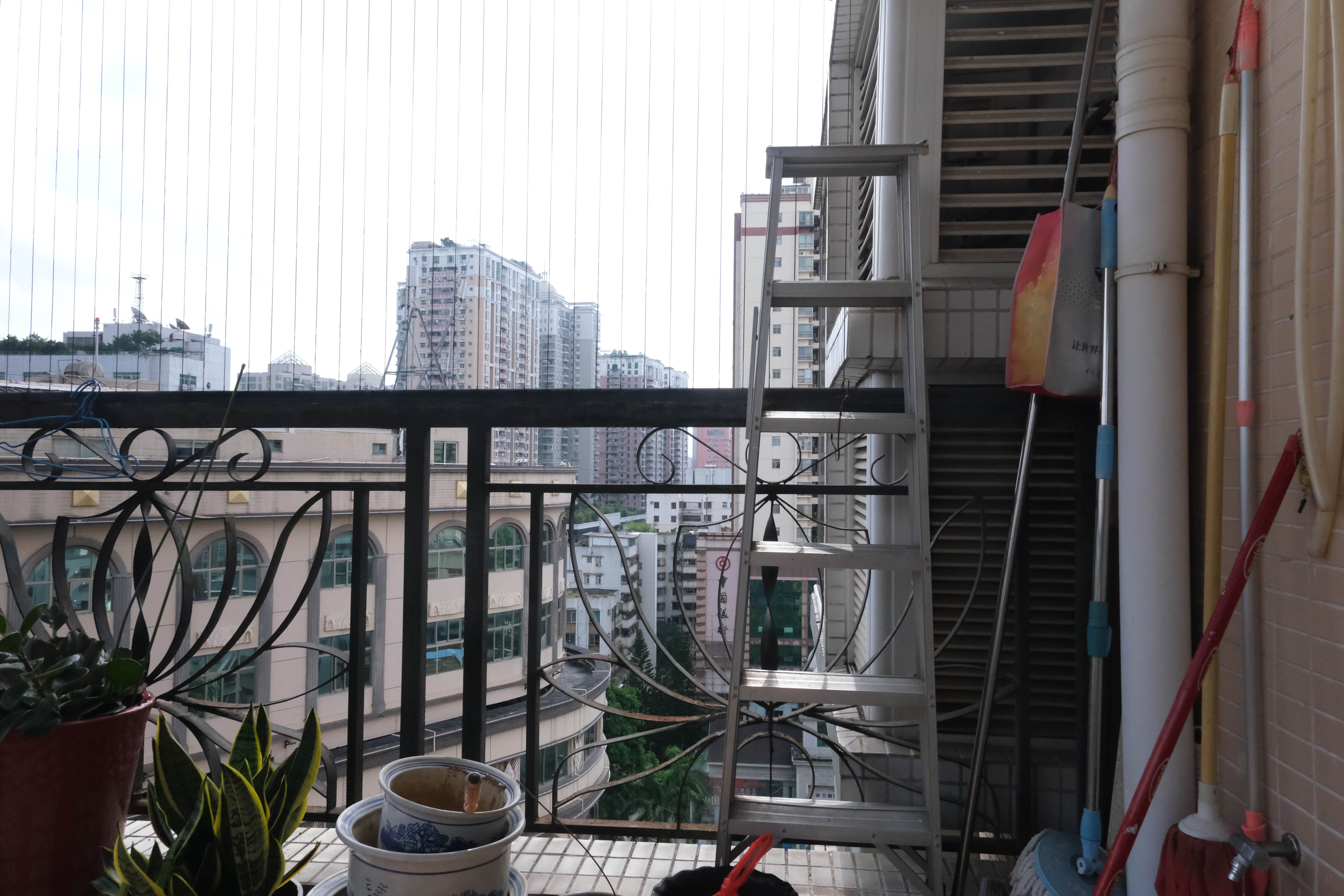
In well-lit situations, vignetting is generally not noticeable. Therefore, we use an ND filter to reduce illumination and capture photos with vignetting. The center light, which passes through an ND filter, travels a shorter distance compared to the light at the edges. This difference in distance contributes to the occurrence of vignetting.

(a)

(b)

(c)
Additionally, to ensure that there is no displacement between each pair of photos and to enhance data diversity, it is crucial to avoid dynamic objects such as swaying tree leaves, moving vehicles, and glass reflections on specific objects that are susceptible to motion. Therefore, we select multiple distinct indoor environments for the data collection. To reduce device vibration caused by manual camera shutter presses, we use remote shutter control to capture steps 2 and 4, as illustrated in Figure 2 (c).
(a)

(b)
Data collection and processing
Figure 2 (a) provides a preview of our experimental configuration designed for capturing VigSet. The process of collecting data is facilitated by adjusting the white ND value controller located on the camera ND filter, as depicted in Figure 2 (c). During the data collection process, we capture images from real-world scenes utilizing experimental equipment. We use a tripod to stabilize the camera and control unrelated variables. The steps of the data collection process are as follows.
-
1.
The camera settings, such as focal length, aperture, exposure, and ISO, are set to fixed values.
-
2.
A vignetting-free image is captured with an ND value of 0, as shown in Figure 3 (a)
-
3.
Continuously modify the value of the ND filter until noticeable vignetting becomes visible in the image.
-
4.
An image with vignetting is captured, as shown in Figure 3 (b)
We exclude images exhibiting obvious motion distortion or lack of focus. Moreover, we conduct group reviews of these photographs to identify and remove any outliers and duplicates.
Methodology
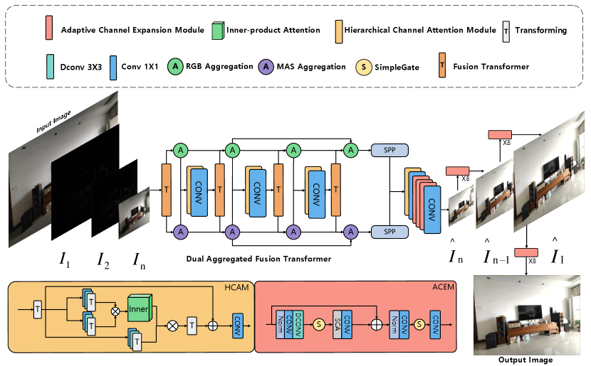
We propose a multi-frequency network based on Dual Aggregated Fusion Transformer with Adaptive Channel Expansion to exploit the features of images at various scales. Specifically, the structure of DeVigNet, as illustrated in Figure 4, includes three major components: The Dual Aggregated Fusion Transformer (DAFT), the Adaptive Channel Expansion Module (ACEM), and the Hierarchical Channel Attention Module (HCAM). In the upcoming sections, we will introduce these components of DeVigNet and the learning criteria.
Dual Aggregated Fusion Transformer
The Dual Aggregated Fusion Transformer (DAFT) is a neural network designed specifically for handling low-frequency information in images. As the foundational architecture, the Fusion Transformer employs multiple attention mechanisms to capture various points of focus, enabling the model to effectively incorporate both local and global information within its representation. Fusion Transformer significantly boosts the expressive capacity of the Transformer network. Figure 4 illustrates the location of these four fusion transformers, wherein each transformer comprises two modules. Each module contains 1, 2, 3, or 4 Transformer Blocks (Dosovitskiy et al. 2021) from left to right. The output of the first module is passed on to the second module, and the final output is obtained by adding the output of the second module to the output of the first module.
Inspired by (Cun, Pun, and Shi 2020), the Aggregation Node is designed as integration operations on the input features. By aggregating the semantic information extracted by the fusion transformer, a richer and more comprehensive global feature representation can be obtained. This Structure facilitates an improved understanding of the image’s structure, texture, and global properties by the model in low frequency, leading to enhancing vignetting removal.
Adaptive Channel Expansion Module
While the primary cause of vignetting is low-frequency color information, some edge information of the images remains. Therefore, motivated by U-Net (Ronneberger, Fischer, and Brox 2015), we propose a structure that integrates Adaptive Contrast Enhancement Module (ACEM) and Laplacian pyramid reconstruction for optimal vignetting removal results in high-frequency.
ACEM is a lightweight module that does not employ any activation functions, and it has been proven that there will be no decrease in performance. Inspired by (Ba, Kiros, and Hinton 2016), the beginning section of ACEM is LayerNorm, which improves stability and reduces computational overhead. The following convolutional layers capture feature information at varying scales. Inspired by (Chen et al. 2022), the Simplified Channel Attention (SCA) and SimpleGate techniques are utilized to enhance network performance. SimpleGate divides the feature maps into two channel dimensions and multiplies them together, leading to a reduction in computational load and complexity. The formula is as follows:
| (1) |
where and are feature maps of the same size. Simplified Channel Attention (SCA) can be considered as a streamlined adaptation of Channel Attention (CA). It captures the essence of CA by retaining only two vital components: aggregating global information and enabling channel-wise interaction. SCA can be described as :
| (2) |
denotes a fully connected layer. represents the global average pooling procedure which combines spatial data into channels. indicates a channel-wise multiplication.
| Methods | LOL | MIT-Adobe FiveK | ||||||
|---|---|---|---|---|---|---|---|---|
| PSNR | SSIM | MAE | LPIPS | PSNR | SSIM | MAE | LPIPS | |
| Input | 7.77 | 0.20 | 99.80 | 0.42 | 12.26 | 0.61 | 55.98 | 0.22 |
| LIME | 16.76 | 0.44 | 30.59 | 0.31 | 13.30 | 0.75 | 52.12 | 0.09 |
| MSRCR | 13.17 | 0.45 | 52.71 | 0.33 | 13.31 | 0.75 | 50.82 | 0.12 |
| NPE | 16.97 | 0.47 | 32.89 | 0.31 | 17.38 | 0.79 | 31.22 | 0.10 |
| WV-SRIE | 11.86 | 0.49 | 65.56 | 0.24 | 18.63 | 0.84 | 26.27 | 0.08 |
| PM-SRIE | 12.28 | 0.51 | 63.28 | 0.23 | 19.70 | 0.84 | 23.42 | 0.07 |
| JieP | 12.05 | 0.51 | 64.34 | 0.22 | 18.64 | 0.84 | 26.42 | 0.07 |
| RetinexNet | 16.77 | 0.42 | 32.02 | 0.38 | 12.51 | 0.69 | 52.73 | 0.20 |
| KID | 17.65 | 0.77 | 31.40 | 0.12 | 16.20 | 0.79 | 35.16 | 0.11 |
| DSLR | 14.98 | 0.60 | 48.90 | 0.27 | 20.24 | 0.83 | 22.45 | 0.10 |
| ELGAN | 17.48 | 0.65 | 34.47 | 0.23 | 16.00 | 0.79 | 36.37 | 0.09 |
| RUAS | 16.40 | 0.50 | 39.11 | 0.19 | 17.91 | 0.84 | 33.12 | 0.08 |
| Zero_DCE | 14.86 | 0.56 | 47.07 | 0.24 | 15.93 | 0.77 | 36.36 | 0.12 |
| Zero_DCE++ | 14.75 | 0.52 | 45.94 | 0.22 | 14.61 | 0.42 | 39.25 | 0.16 |
| Uformer | 18.55 | 0.73 | 28.91 | 0.23 | 21.92 | 0.87 | 17.91 | 0.06 |
| Ours | 21.33 | 0.76 | 19.30 | 0.16 | 23.10 | 0.84 | 15.43 | 0.16 |
Hierarchical Channel Attention Module
Inspired by (Wang et al. 2023), The Hierarchical Channel Attention Module (HCAM) module is dedicated to the hierarchical fusion of features and the acquisition of learnable correlations across diverse layers. The primary function of HCAM is to compute and apply attention weights to the input feature map, resulting in the refinement and enhancement of vignetting features. Initially, HCAM performs a transformation on the input to yield , from successive layers. Subsequently, the (query), (key), and (value) features are extracted using convolutional layers. Subsequently, the , , and features are extracted using convolutional layers.
In this module, Inner-Product Attention plays a crucial role in calculating attention scores by computing the dot product between the query and the key. HCAM adaptively fuses features from different hierarchical levels by conducting weighted operations between values and attention scores. The corresponding output feature can be described as:
| (3) |
where represents Layer Attention, indicates Convolution , can be written as:
| (4) |
Learning Criteria
During the training phase, we employ two loss functions, namely Mean Squared Error () and Structural Similarity Index Measure () (Wang et al. 2004), which offer significant advantages in preserving the intricate details of the image. The mathematical expressions for these losses are as follows:
| (5) |
The weight of is empirically set to 0.4.
Experiments
Methods PSNR SSIM MAE LPIPS PSNR SSIM MAE LPIPS PSNR SSIM MAE LPIPS Input 12.08 0.59 60.04 0.18 12.08 0.58 60.04 0.18 12.08 0.58 60.04 0.19 RIVC 13.08 0.59 55.17 0.18 13.08 0.59 55.17 0.18 13.08 0.59 55.17 0.19 SIVC 14.65 0.62 43.71 0.17 14.65 0.61 43.69 0.17 14.65 0.60 43.70 0.18 LIME 12.42 0.41 51.29 0.41 12.42 0.39 51.29 0.40 12.41 0.37 51.32 0.42 MSRCR 11.20 0.39 60.43 0.44 11.20 0.37 60.43 0.45 11.20 0.35 60.44 0.46 NPE 15.72 0.51 38.60 0.33 15.72 0.49 38.59 0.32 15.72 0.47 38.60 0.33 WV-SRIE 18.84 0.60 26.67 0.22 18.84 0.58 26.67 0.23 18.84 0.56 26.67 0.24 PM-SRIE 19.45 0.66 24.81 0.16 19.45 0.64 24.81 0.17 19.45 0.62 24.81 0.19 JieP 18.93 0.58 26.33 0.24 18.93 0.55 26.32 0.25 18.93 0.54 26.32 0.27 KID 14.73 0.71 44.01 0.18 14.74 0.71 43.95 0.22 14.73 0.71 44.00 0.31 DSLR 19.37 0.65 24.10 0.16 19.37 0.64 24.07 0.20 19.35 0.62 24.10 0.29 ELGAN 16.32 0.73 37.77 0.10 16.32 0.72 37.76 0.11 16.31 0.72 37.77 0.12 RUAS 15.54 0.60 36.93 0.22 15.54 0.57 36.92 0.24 15.54 0.56 36.92 0.25 Zero-DCE 16.28 0.58 34.77 0.26 16.28 0.57 34.77 0.26 16.28 0.55 34.78 0.26 Zero-DCE++ 16.82 0.55 32.31 0.20 16.82 0.52 32.32 0.21 16.81 0.51 32.34 0.23 Uformer 20.95 0.77 21.32 0.19 20.60 0.77 22.80 0.25 20.67 0.77 22.69 0.28 Ours 22.96 0.79 15.82 0.09 22.94 0.78 15.84 0.11 22.94 0.77 15.85 0.13
Ablation Study PSNR SSIM MAE LPIPS PSNR SSIM MAE LPIPS PSNR SSIM MAE LPIPS Input 12.08 0.59 60.04 0.18 12.08 0.58 60.04 0.18 12.08 0.58 60.04 0.19 Ours w/ Depth=3 16.04 0.69 32.44 0.16 16.04 0.69 32.44 0.17 16.04 0.70 32.44 0.19 Ours w/ Depth=4 13.94 0.66 42.62 0.21 13.94 0.67 42.63 0.23 13.94 0.68 42.63 0.22 Ours w/o ACEM 19.66 0.76 23.77 0.11 19.66 0.74 23.78 0.14 19.65 0.74 23.79 0.17 Ours w/o DAFT 18.25 0.73 28.75 0.14 18.25 0.72 28.75 0.15 18.25 0.72 28.75 0.16 DHAN w/ ACEM 21.84 0.75 17.73 0.20 20.95 0.74 19.96 0.21 21.13 0.74 19.25 0.23 Ours 22.96 0.79 15.82 0.09 22.94 0.78 15.84 0.11 22.94 0.77 15.85 0.13

(a) Input

(b) ELGAN

(c) UFormer

(d) Zero-DCE

(e) RIVC

(f) SIVC

(g) Ours

(h) Target
(a) Input

(b) ELGAN

(c) UFormer

(d) Zero-DCE

(e) LIME

(f) NPE

(g) Ours

(h) Target
Experiment Settings
In order to ensure the highest level of fidelity and reliability in our experiments, we have made the deliberate decision to exclusively use the VigSet dataset for vignetting removal. Moreover, we also conduct experiments in the field of LLIE to demonstrate the versatility of DeVigNet in global illuminance adjustment.
In our experiments, we leverage the following datasets:
VigSet: This dataset contains 983 image pairs. We allocate 803 pairs for training purposes and reserve the remaining 180 pairs for testing.
MIT-Adobe FiveK (Bychkovsky et al. 2011) & LOL-v1 (Wei et al. 2018): For these datasets, we adopt the experimental settings delineated in (Wang et al. 2023), ensuring consistency with prior research.
Evaluation Metrics
We evaluate the quality of the enhanced images using four widely adopted metrics: Peak Signal-to-Noise Ratio (PSNR), Structural Similarity (SSIM), Mean Absolute Error (MAE). In addition, to better align with human perceptual conditions, we utilize the Learned Perceptual Image Patch Similarity (LPIPS). These metrics are commonly used in the assessment of image enhancement and low-level computer vision tasks. Higher PSNR and SSIM scores indicate improved visual quality, while lower MAE and LPIPS suggest better accuracy in representing the original image.
Implementation Details
We employ PyTorch to implement our model and conduct experiments using the NVIDIA A40 GPU. We utilize the Adam optimizer, adhering to its default parameter settings. During the training process, all models are trained at a resolution of and subsequently tested at different resolutions. Additionally, we set the batch size to 1 and the learning rate to .
Comparisons with State-of-the-Art
We have performed a comprehensive evaluation of state-of-the-art vignetting removal methods on the VigSet dataset. The compared vignetting methods include SIVC (Zheng et al. 2008) and RIVC (Lopez-Fuentes, Oliver, and Massanet 2015). These methods serve as benchmarks for evaluating the performance of our proposed vignetting removal technique.
Furthermore, we also conduct additional experiments with state-of-the-art LLIE methods. We compare DeVigNet with traditional LLIE methods such as LIME (Guo, Li, and Ling 2016), MSRCR (Jobson, Rahman, and Woodell 1997), and NPE (Wang et al. 2013). Additionally, we evaluate the performance of learning-based LLIE methods, including WV-SRIE (Fu et al. 2016), PM-SRIE (Fu et al. 2015), Uformer (Wang et al. 2022), KID (Zhang, Zhang, and Guo 2019), DSLR (Lim and Kim 2020), ELGAN (Jiang et al. 2021), JieP (Cai et al. 2017), RUAS (Liu et al. 2021), Zero-DCE (Guo et al. 2020), and Zero-DCE++ (Li, Guo, and Loy 2021).
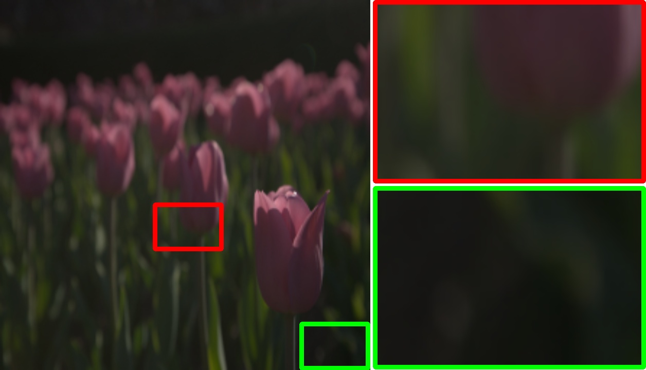
Qualitative results, as shown in Figure 5 demonstrate that our method exhibits significant superiority over others in the vignetting dataset. Our results display enhanced image clarity and more prominent vignetting removal. Moreover, our method achieves competitiveness on the LLIE dataset as shown in Figure 6.
In terms of quantitative results, by comparing our proposed method with these state-of-the-art vignetting and LLIE methods as displayed in Table 1 and Table 2, we can assess its effectiveness and performance in relation to existing methods. This comprehensive evaluation provides insights into the strengths and weaknesses of different approaches and helps to advance the field of vignetting removal.
Conventional methods heavily depend on assumptions based on physics, which are not consistently accurate. Additionally, current LLIE methods are not well-suited for addressing the issue of vignetting. Therefore, based on the data from Table 2, it is evident that traditional methods and LLIE methods exhibit substantial disparities compared to other methods in multiple metrics, particularly in terms of MAE. Additionally, we conducted supplementary quantitative experiments on a LLIE dataset, as presented in Table 1. The results illustrate the strong performance of our method in LLIE. Besides, with the advancement of current technology, capturing high-resolution images has become an essential routine. DeVigNet stands out as the most efficient approach in achieving superior results in vignetting removal across various resolutions when compared to other existing methods.
Ablation Studies
We maintain a similar parameter count across all combinations to ensure a fair comparison. DAFT and ACEM are removed respectively using the comment-out method in the experiments. As shown in Table 3, we conduct ablation studies evaluating various components of our model at different image resolutions. These components include varying the depth of the Laplacian pyramid, as well as ablating the ACEM and DAFT modules.
As the depth of the Laplacian pyramid increases, the magnitude of the low-frequency component decreases. This reduction directly impacts the quality of vignetting removal, especially with respect to preserving low-frequency color information.
DAFT plays a pivotal role in capturing global color information within the low-frequency component of an image. Therefore, models lacking DAFT suffer performance degradation due to the loss of global color context.
Meanwhile, ACEM is primarily utilized to retain edge details during image reconstruction, focusing on the high-frequency portion. Removing ACEM causes models to lose textural information in the reconstruction phase, thereby deteriorating performance due to the absence of high-frequency context.
Additionally, we replace DAFT with DHAN (Cun, Pun, and Shi 2020), the results are shown in Table 3. Accordingly, DAFT and ACEM are responsible for the low-frequency and high-frequency components, respectively. While each component contributes individually to improved vignetting removal performance, their combined effect yields optimal results by leveraging complementary global and local context.
Conclusion
In this paper, we introduce Vigset, the first large-scale high-resolution vignetting removal dataset with ground truth images. Vigset comprises 983 pairs of images captured under different lighting conditions and in various scenes. Additionally, we propose a novel method called DeVigNet, specifically designed for vignetting removal on this dataset. It includes three components: The Dual Aggregated Fusion Transformer, the Adaptive Channel Expansion Module and the Hierarchical Channel Attention Module. By utilizing the Laplacian pyramid, DeVigNet performs vignetting removal on the color information in the high-frequency and low-frequency domains of the image, thereby achieving optimal results. DeVigNet effectively eliminates vignetting effects in images, demonstrating superior performance compared to existing methods in terms of both quality and quantity for vignetting removal.
Acknowledgement
This work was supported in part by the Science and Technology Development Fund, Macau SAR, under Grant 0087/2020/A2 and Grant 0141/2023/RIA2, in part by the National Natural Science Foundations of China under Grant 62172403, in part by the Distinguished Young Scholars Fund of Guangdong under Grant 2021B1515020019, in part by the Excellent Young Scholars of Shenzhen under Grant RCYX20200714114641211.
References
- Ba, Kiros, and Hinton (2016) Ba, J. L.; Kiros, J. R.; and Hinton, G. E. 2016. Layer normalization. arXiv preprint arXiv:1607.06450.
- Burt and Adelson (1987) Burt, P. J.; and Adelson, E. H. 1987. The Laplacian pyramid as a compact image code. In Readings in computer vision, 671–679. Elsevier.
- Bychkovsky et al. (2011) Bychkovsky, V.; Paris, S.; Chan, E.; and Durand, F. 2011. Learning photographic global tonal adjustment with a database of input/output image pairs. In CVPR, 97–104.
- Cai et al. (2017) Cai, B.; Xu, X.; Guo, K.; Jia, K.; Hu, B.; and Tao, D. 2017. A joint intrinsic-extrinsic prior model for retinex. In Proceedings of the IEEE international conference on computer vision, 4000–4009.
- Chen et al. (2022) Chen, L.; Chu, X.; Zhang, X.; and Sun, J. 2022. Simple baselines for image restoration. In European Conference on Computer Vision, 17–33. Springer.
- Cun, Pun, and Shi (2020) Cun, X.; Pun, C.-M.; and Shi, C. 2020. Towards ghost-free shadow removal via dual hierarchical aggregation network and shadow matting gan. In Proceedings of the AAAI Conference on Artificial Intelligence, 10680–10687.
- Dosovitskiy et al. (2021) Dosovitskiy, A.; Beyer, L.; Kolesnikov, A.; Weissenborn, D.; Zhai, X.; Unterthiner, T.; Dehghani, M.; Minderer, M.; Heigold, G.; Gelly, S.; Uszkoreit, J.; and Houlsby, N. 2021. An Image is Worth 16x16 Words: Transformers for Image Recognition at Scale. ICLR.
- Fu et al. (2015) Fu, X.; Liao, Y.; Zeng, D.; Huang, Y.; Zhang, X.-P.; and Ding, X. 2015. A probabilistic method for image enhancement with simultaneous illumination and reflectance estimation. IEEE Transactions on Image Processing, 24(12): 4965–4977.
- Fu et al. (2016) Fu, X.; Zeng, D.; Huang, Y.; Zhang, X.-P.; and Ding, X. 2016. A weighted variational model for simultaneous reflectance and illumination estimation. In Proceedings of the IEEE conference on computer vision and pattern recognition, 2782–2790.
- Goldman (2010) Goldman, D. B. 2010. Vignette and exposure calibration and compensation. IEEE transactions on pattern analysis and machine intelligence, 32(12): 2276–2288.
- Guo et al. (2020) Guo, C.; Li, C.; Guo, J.; Loy, C. C.; Hou, J.; Kwong, S.; and Cong, R. 2020. Zero-reference deep curve estimation for low-light image enhancement. In Proceedings of the IEEE/CVF conference on computer vision and pattern recognition, 1780–1789.
- Guo, Li, and Ling (2016) Guo, X.; Li, Y.; and Ling, H. 2016. LIME: Low-light image enhancement via illumination map estimation. IEEE TIP, 26(2): 982–993.
- Jiang et al. (2021) Jiang, Y.; Gong, X.; Liu, D.; Cheng, Y.; Fang, C.; Shen, X.; Yang, J.; Zhou, P.; and Wang, Z. 2021. Enlightengan: Deep light enhancement without paired supervision. IEEE TIP, 30: 2340–2349.
- Jobson, Rahman, and Woodell (1997) Jobson, D.; Rahman, Z.; and Woodell, G. 1997. A multiscale retinex for bridging the gap between color images and the human observation of scenes. IEEE Transactions on Image Processing, 6(7): 965–976.
- Li, Guo, and Loy (2021) Li, C.; Guo, C.; and Loy, C. C. 2021. Learning to enhance low-light image via zero-reference deep curve estimation. IEEE Transactions on Pattern Analysis and Machine Intelligence, 44(8): 4225–4238.
- Li et al. (2023a) Li, Z.; Chen, X.; Pun, C.-M.; and Cun, X. 2023a. High-Resolution Document Shadow Removal via A Large-Scale Real-World Dataset and A Frequency-Aware Shadow Erasing Net. In Proceedings of the IEEE/CVF International Conference on Computer Vision (ICCV), 12449–12458.
- Li et al. (2023b) Li, Z.; Chen, X.; Wang, S.; and Pun, C.-M. 2023b. A Large-Scale Film Style Dataset for Learning Multi-frequency Driven Film Enhancement. In Proceedings of the Thirty-Second International Joint Conference on Artificial Intelligence, IJCAI-23, 1160–1168.
- Liang, Zeng, and Zhang (2021) Liang, J.; Zeng, H.; and Zhang, L. 2021. High-resolution photorealistic image translation in real-time: A laplacian pyramid translation network. In Proceedings of the IEEE/CVF Conference on Computer Vision and Pattern Recognition, 9392–9400.
- Lim and Kim (2020) Lim, S.; and Kim, W. 2020. Dslr: Deep stacked laplacian restorer for low-light image enhancement. IEEE TMM, 23: 4272–4284.
- Liu et al. (2021) Liu, R.; Ma, L.; Zhang, J.; Fan, X.; and Luo, Z. 2021. Retinex-inspired unrolling with cooperative prior architecture search for low-light image enhancement. In CVPR, 10561–10570.
- Lopez-Fuentes, Oliver, and Massanet (2015) Lopez-Fuentes, L.; Oliver, G.; and Massanet, S. 2015. Revisiting image vignetting correction by constrained minimization of log-intensity entropy. In Advances in Computational Intelligence: 13th International Work-Conference on Artificial Neural Networks, IWANN 2015, Palma de Mallorca, Spain, June 10-12, 2015. Proceedings, Part II 13, 450–463. Springer.
- Ronneberger, Fischer, and Brox (2015) Ronneberger, O.; Fischer, P.; and Brox, T. 2015. U-net: Convolutional networks for biomedical image segmentation. In Medical Image Computing and Computer-Assisted Intervention–MICCAI 2015: 18th International Conference, Munich, Germany, October 5-9, 2015, Proceedings, Part III 18, 234–241. Springer.
- Wang et al. (2013) Wang, S.; Zheng, J.; Hu, H.-M.; and Li, B. 2013. Naturalness Preserved Enhancement Algorithm for Non-Uniform Illumination Images. IEEE Transactions on Image Processing, 22(9): 3538–3548.
- Wang et al. (2023) Wang, T.; Zhang, K.; Shen, T.; Luo, W.; Stenger, B.; and Lu, T. 2023. Ultra-high-definition low-light image enhancement: a benchmark and transformer-based method. In Proceedings of the AAAI Conference on Artificial Intelligence, volume 37, 2654–2662.
- Wang et al. (2004) Wang, Z.; Bovik, A. C.; Sheikh, H. R.; and Simoncelli, E. P. 2004. Image quality assessment: from error visibility to structural similarity. IEEE transactions on image processing, 13(4): 600–612.
- Wang et al. (2022) Wang, Z.; Cun, X.; Bao, J.; and Liu, J. 2022. Uformer: A general u-shaped transformer for image restoration. In CVPR, 17683–17693.
- Wei et al. (2018) Wei, C.; Wang, W.; Yang, W.; and Liu, J. 2018. Deep retinex decomposition for low-light enhancement. In BMVC.
- You et al. (2022) You, S.; Lei, B.; Wang, S.; Chui, C. K.; Cheung, A. C.; Liu, Y.; Gan, M.; Wu, G.; and Shen, Y. 2022. Fine perceptive gans for brain mr image super-resolution in wavelet domain. IEEE transactions on neural networks and learning systems.
- Zhang, Zhang, and Guo (2019) Zhang, Y.; Zhang, J.; and Guo, X. 2019. Kindling the darkness: A practical low-light image enhancer. In ACMMM, 1632–1640.
- Zheng et al. (2013) Zheng, Y.; Lin, S.; Kang, S. B.; Xiao, R.; Gee, J. C.; and Kambhamettu, C. 2013. Single-Image Vignetting Correction from Gradient Distribution Symmetries. IEEE Trans Pattern Anal Mach Intell, 35(6): 1480–1494.
- Zheng et al. (2008) Zheng, Y.; Yu, J.; Kang, S. B.; Lin, S.; and Kambhamettu, C. 2008. Single-image vignetting correction using radial gradient symmetry. In 2008 IEEE Conference on Computer Vision and Pattern Recognition, 1–8. IEEE.