Deterministic $k$ -Vertex Connectivity in $k^{2}$ Max-flows

Chaitanya Nalam [email protected]. University of Michigan, USA Thatchaphol Saranurak [email protected]. University of Michigan, USA. Supported by NSF CAREER grant 2238138. Sorrachai Yingchareonthawornchai [email protected]. Aalto University, Finland

Abstract

An $n$ -vertex $m$ -edge graph is $k$ -vertex connected if it cannot be disconnected by deleting less than $k$ vertices. After more than half a century of intensive research, the result by [Li et al. STOC’21] finally gave a randomized algorithm for checking $k$ -connectivity in near-optimal $\widehat{O}(m)$ time.¹¹1We use $\widehat{O}(\cdot)$ to hide an $n^{o(1)}$ factor. Deterministic algorithms, unfortunately, have remained much slower even if we assume a linear-time max-flow algorithm: they either require at least $\Omega(mn)$ time [Even’75; Henzinger Rao and Gabow, FOCS’96; Gabow, FOCS’00] or assume that $k=o(\sqrt{\log n})$ [Saranurak and Yingchareonthawornchai, FOCS’22].

We show a deterministic algorithm for checking $k$ -vertex connectivity in time proportional to making $\widehat{O}(k^{2})$ max-flow calls, and, hence, in $\widehat{O}(mk^{2})$ time using the deterministic max-flow algorithm by [Brand et al. FOCS’23]. Our algorithm gives the first almost-linear-time bound for all $k$ where $\sqrt{\log n}\leq k\leq n^{o(1)}$ and subsumes up to a sub polynomial factor the long-standing state-of-the-art algorithm by [Even’75] which requires $O(n+k^{2})$ max-flow calls.

Our key technique is a deterministic algorithm for terminal reduction for vertex connectivity: given a terminal set separated by a vertex mincut, output either a vertex mincut or a smaller terminal set that remains separated by a vertex mincut.

We also show a deterministic $(1+\epsilon)$ -approximation algorithm for vertex connectivity that makes $O(n/\epsilon^{2})$ max-flow calls, improving the bound of $O(n^{1.5})$ max-flow calls in the exact algorithm of [Gabow, FOCS’00]. The technique is based on Ramanujan graphs.

1 Introduction

Vertex connectivity of an $n$ -vertex $m$ -edge undirected graph $G$ , denoted by $\kappa_{G}$ , is the minimum number of vertices to be removed to disconnect the graph (or to become a singleton). Vertex connectivity along with its related problem called edge connectivity (where we remove edges to disconnect the graph) are both fundamental and very well-studied problems in graph algorithm research [Men27, Kle69, Pod73, ET75, Eve75, Gal80, EH84, Mat87, BDD⁺82, LLW88, CT91, NI92, CR94, Hen97, HRG00, Gab06, CGK14], see [NSY19] for more discussion. The complexity of the edge connectivity problem is well-understood: It can be solved in nearly linear time using randomization by Karger since 2000 [Kar00] and, more recently, it can also be solved deterministically in near-linear time [KT15, HRW17] and even in weighted case [LP20, Li21].

For vertex connectivity, there is still a large gap in our understanding. Aho, Hopcroft, and Ullman asked almost 50 years ago if vertex connectivity can be solved in linear time [AHU74]. The answer is affirmative (up to a subpolynomial factor) using randomization: Recent developments [NSY19, FNS⁺20, LNP⁺21] culminate in a celebrated “polylog max-flow” time, which is almost linear by the recent breakthrough in max-flow problem [CKL⁺22].

Deterministic algorithms, on the other hand, have remained much slower. In the discussion below, we will assume a linear-time deterministic max-flow algorithm so that we can highlight the development of ideas related to vertex connectivity itself and not about the implementation of max-flow algorithms. This is actually without loss of generality because Brand et al. [BCG⁺23] recently showed an almost-linear-time deterministic max-flow algorithm. Let us consider the problem of checking $k$ -vertex connectivity (i.e., deciding if vertex connectivity is at least $k$ or outputs a minimum vertex cut).²²2Note that, for all results stated below including our results, we can assume that $m=O(nk)$ by using the linear-time sparsification algorithm by [NI92]. When $k\leq 3$ , $O(m)$ -time algorithms are known using a depth-first search [Tar72] and a data structure called SPQR tree [HT73]. Very recently, [SY22] showed an $\widehat{O}(m2^{O(k^{2})})$ -time algorithm which is almost-linear for all $k=o(\sqrt{\log n})$ . For general $k$ , half a century ago, Kleitman [Kle69] showed an algorithm that makes $O(nk)$ max-flow calls. Then, Even [Eve75] improved the number of max-flow calls to $O(n+k^{2})$ . [HRG00] later showed how to implement the first $n$ calls to max-flow in Even’s algorithm in $O(mn)$ time, without assuming a linear-time max-flow algorithm. The currently fastest deterministic algorithm is by Gabow [Gab06]. The bound stated in his paper is $O(\min\{n^{3/4},k^{1.5}\}km+mn)$ time, but this bound is based on max-flow algorithms that are slower than linear time. One can show that his algorithms take time proportional to $O(n+k\min\{k,\sqrt{n}\})$ max flow calls, which improved upon Even’s algorithm when $k\geq\sqrt{n}$ .

To summarize state of the art, for any $k\geq\sqrt{\log n}$ , all known deterministic algorithms require $\Omega(n)$ max-flow calls, which is $\Omega(mn)$ time even if we assume a linear time max-flow algorithm.

1.1 Our Results

In this paper, we show a deterministic algorithm for checking $k$ -vertex connectivity in $\widehat{O}(k^{2})$ max-flows. Let $G=(V,E)$ be an undirected graph. A vertex cut $(L,S,R)$ is a partition of the vertex set $V$ such that there is no edge between $L$ and $R$ . The size of $(L,S,R)$ is $|S|$ .

Theorem 1.1.

There is a deterministic algorithm that takes as inputs an $n$ -vertex $m$ -edge undirected graph $G=(V,E)$ , and connectivity parameter $k$ , and either outputs a vertex cut of size less than $k$ or concludes that $G$ is $k$ -vertex connected. The algorithm makes calls to unit-vertex-capacity max-flow instances with $\widehat{O}(mk^{2})$ number of edges in total and spends an additional $\widehat{O}(mk^{2})$ time.

In particular, our algorithm runs in $o(n)$ max-flows whenever $k\ll\sqrt{n}$ . This is the first algorithm that improves the long-standing state-of-the-art algorithm [Eve75] that runs in $O(n+k^{2})$ max-flows. Using the almost linear time deterministic max-flow algorithm [BCG⁺23], our algorithm runs in $\widehat{O}(mk^{2})$ time, which is the fastest whenever $k\ll\sqrt{n}$ . Our algorithm exponentially improves the dependency on $k$ from the recent $\widehat{O}(m2^{O(k^{2})})$ -time algorithm [SY22].

We also show a $(1+\epsilon)$ -approximation algorithm for computing vertex connectivity of $G$ , $\kappa_{G}$ .

Theorem 1.2.

There is a deterministic algorithm that takes an $n$ -vertex $m$ -edge undirected graph $G$ and accuracy parameter $\epsilon\in(0,1)$ as inputs and outputs a vertex cut of size at most $\lfloor(1+\epsilon)\kappa_{G}\rfloor$ . The algorithm makes $O(n/\epsilon^{2})$ calls to unit-vertex-capacity $(s,t)$ -max-flows on $G$ and spends additional $O(n/\epsilon^{2})$ time.

In particular, this algorithm runs in $\widehat{O}(\frac{1}{\epsilon^{2}}\cdot mn)$ time using the max-flow algorithm by [BCG⁺23]. This is the first deterministic approximation algorithm that runs in $\ll mn^{1.5}$ time, and improves upon the exact algorithm [Gab06] that requires $n^{1.5}$ max-flows in the general case.

1.2 Techniques

The key to our result is the terminal reduction algorithm for vertex connectivity that runs in $\widehat{O}(k^{2})$ max-flows. Let $G=(V,E)$ be an $n$ -vertex $m$ -edge undirected graph with terminal set $T\subseteq V$ . A $T$ -Steiner vertex cut $(L,S,R)$ is a vertex cut such that $T\cap L\neq\emptyset$ and $T\cap R\neq\emptyset$ . We denote $\kappa_{G}(T)$ as the size of the minimum $T$ -Steiner vertex cut in $G$ or $n-1$ if it does not exist. By definition, vertex connectivity of $G$ , denoted by $\kappa_{G}$ is equal to $\kappa_{G}(V)$ . We omit the subscript when the context is clear. Our main technical result is:

Theorem 1.3 (Terminal reduction).

There is a deterministic algorithm that takes as inputs an $n$ -vertex $m$ -edge undirected graph $G=(V,E)$ , along with a terminal set $T\subseteq V$ and a cut parameter $k$ , and outputs either a vertex cut of size less than $k$ or a new terminal set $T^{\prime}\subseteq V$ of size at most $|T|/2$ such that $\kappa(T^{\prime})<k$ if $\kappa(T)<k$ . The algorithm makes calls to unit-vertex-capacity max-flow instances with $\widehat{O}(mk^{2})$ number of edges in total and spends an additional $\widehat{O}(mk^{2})$ time.

Intuitively, terminal reduction means we find a smaller terminal set $T^{\prime}$ such that the minimum $T$ -Steiner cut of size less than $k$ remains $T^{\prime}$ -Steiner. Given Theorem 1.3, our main theorem follows immediately.

Proof of Theorem 1.1.

To check $k$ -vertex connectivity of a graph $G=(V,E)$ , we start with the entire vertex set $V$ as a terminal set, and repeatedly apply Theorem 1.3 for $O(\log n)$ times until we obtain a vertex cut of size less than $k$ or the terminal set becomes empty ( $T=\emptyset$ ) for which we conclude that $G$ is $k$ -vertex connected. ∎

Prior to our work, [LP20] (implicitly) showed exactly the same terminal reduction algorithm as in Theorem 1.3 except their algorithm is for edge mincuts and they guaranteed that $T^{\prime}\subseteq T$ , i.e., the output terminal $T^{\prime}$ is always a subset of the input terminal $T$ . This is not guaranteed by our Theorem 1.3.

Terminal Reduction Framework.

The key method to the proof of Theorem 1.3 is to generalize the vertex reduction framework in [SY22] to the terminal setting. At a high-level, the vertex reduction framework in [SY22] consists of two steps.

1.

First, given a graph $G=(V,E)$ , their algorithm outputs either a vertex cut of size $<k$ or a terminal set $T\subseteq V$ of size $\ll n$ such that $\kappa_{G}(T)<k$ iff $\kappa_{G}<k$ .
2.

In the second step, which is a vertex reduction step, given the terminal set $T$ from the first step, their algorithm outputs a smaller graph $H$ of size $\widehat{O}(|T|)<m/2$ such that $\kappa_{G}<k$ iff $\kappa_{H}<k$ .

The two-step vertex reduction framework [SY22] allows them to solve $k$ -vertex connectivity after repeatedly applying it for $O(\log n)$ times. The drawback in their algorithm is that their second step requires $\widehat{O}(m2^{O(k^{2})})$ time, which is very slow when $k\gg\sqrt{\log n}$ .

In this paper, we consider the generalization, of the first step of the vertex reduction framework [SY22], to the terminal setting:

Given a graph $G=(V,E)$ and its terminal set $T\subseteq V$ , output either a vertex cut of size less than $k$ or a terminal set $T^{\prime}$ of size at most $|T|/2$ such that $\kappa(T^{\prime})<k$ iff $\kappa(T)<k$ .

As a result, the new algorithm bypasses the second step of the vertex reduction framework [SY22] by directly reducing the terminal set while maintaining the Steiner connectivity of the output terminal set. Thus, we avoid spending $\widehat{O}(m2^{O(k^{2})})$ time for vertex reduction as in [SY22]. By Theorem 1.3, we only spend $\widehat{O}(mk^{2})$ time instead (using a deterministic linear-time max-flow algorithm [BCG⁺23]). The bottleneck of $k^{2}$ factor stems from the key subroutine in our terminal reduction that handles terminal-unbalanced vertex cuts which we discuss next. We say that a vertex cut $(L,S,R)$ is terminal-unbalanced if $\min\{|T\cap L|,|T\cap R|\}\leq n^{o(1)}$ .

Handling Terminal-unbalanced Vertex Cuts.

For simplicity, consider the following task:

Given a terminal set $T\subseteq V$ with a promised that there is a vertex cut $(L,S,R)$ of size less than $k$ such that $|T\cap L|=1,|T\cap R|\geq 1$ , design a fast algorithm that outputs a vertex cut of size less than $k$ .

If the vertex cut $(L,S,R)$ with the above promise is such that $S\cap T=\emptyset$ , then we say that $(L,S,R)$ isolates $T$ . In this case, we can apply the isolating vertex cut lemma [LNP⁺21] to deterministically output a vertex cut of size less than $k$ in time proportional to $O(\log|T|)$ calls of max-flows and we are done. In general, the vertex cut $(L,S,R)$ may not be $T$ -isolating because possibly $S\cap T\neq\emptyset$ . As a result, it remains to solve the following task.

Find a subset $T^{\prime}\subseteq T$ where $(L,S,R)$ isolates $T^{\prime}$ , i.e., $|T^{\prime}\cap L|=1,|T^{\prime}\cap S|=0,|T^{\prime}\cap R|\geq 1$ .

To do so, we construct a family $\mathcal{F}$ of subsets $U\subseteq T$ of size $|\mathcal{F}|\leq k^{2}\log^{O(1)}n$ such that $(L,S,R)$ must isolate some $U^{\prime}\in\mathcal{F}$ via a Hit and miss hash family [KP20]. Given such a family $\mathcal{F}$ , we apply the isolating vertex cut lemma on each $U\in\mathcal{F}$ to obtain a vertex cut of size less than $k$ as desired. The total running time is roughly $k^{2}\log^{O(1)}n\cdot O(\log|T|)=k^{2}\log^{O(1)}n$ calls to max-flows.

Using Ramanujan graphs for Approximate Mincuts.

The goal is to find a vertex cut of size at most $(1+\epsilon)\kappa_{G}$ . If the minimum degree is at most $(1+\epsilon)\kappa_{G}$ , we can simply return the neighbor set of the min-degree vertex, sacrificing a $(1+\epsilon)$ factor. Otherwise, it is easy to show that any minimum cut $(L,S,R)$ is such that $|L|,|R|\geq\epsilon\kappa_{G}$ , i.e., the cut is quite balanced. We show that Ramanujan graphs can give us a list of $O(n/\epsilon^{2})$ vertex pairs such that a pair $(s,t)$ must exist where $s\in L,t\in R$ . Thus, we will identify a minimum vertex cut by running unit-vertex-capacity $(s,t)$ -max-flows on graph $G$ for each of the $O(n/\epsilon^{2})$ vertex pairs.

To obtain the above list of vertex pairs, let $X=(V,E_{X})$ be a regular Ramanujan graph with degree $\Theta(1/\epsilon^{2})$ . Assuming $|L|\leq|R|$ , we want to show that there exists an edge $(s,t)\in E_{X}$ where $s\in L$ and $t\in R$ . There are two cases. If $|L|\geq\Omega(\epsilon n)$ , then such an edge $(s,t)\in E_{X}$ must exist by the expander mixing lemma as observed before in [Gab06]. Otherwise, we use the known fact that strong spectral expansion of $X$ implies strong vertex expansion for all “small” sets of $X$ . Since $|L|\leq O(\epsilon n)$ , one can show that the vertex expansion of $L$ is at least $2/\epsilon$ , that is $|N_{X}(L)|\geq 2|L|/\epsilon\geq 2\kappa_{G}$ where $N_{X}(L)$ denotes the set of neighbors of $L$ in $X$ . So $N_{X}(L)\setminus(L\cup S)\neq\emptyset$ , i.e., $N_{X}(L)\cap R\neq\emptyset$ . This again implies an edge $(s,t)\in E_{X}$ where $s\in L$ and $t\in R$ .

1.3 Organization

We start with introducing the notations needed for the rest of the paper in Section 2. In Section 3, we prove our main technical result which is the fast terminal reduction algorithm (Theorem 1.3) that implies our main result Theorem 1.1. In Section 4, we use the Ramanujan expanders to obtain a faster approximation algorithm, proving Theorem 1.2.

2 Preliminaries

When we say a graph $G=(V,E)$ , we denote $n=|V|$ and $m=|E|$ unless stated otherwise. Let $A,B\subseteq V$ , we use $E(A,B)$ to denote the set of edges whose one endpoint belongs to $A$ and the other belongs to $B$ . For the rest of the paper, unless stated otherwise, when we say an algorithm, we mean a deterministic algorithm. When we say $k$ -connected, we mean $k$ -vertex connected. When we say a cut, we mean vertex cut.

For any vertex set $S$ , we denote $G-S$ as the graph $G$ after removing all vertices in $S$ . A vertex cut $(L,S,R)$ is a partition of the vertex set $V$ such that there is no edge between $L$ and $R$ . We say that a vertex set $S$ is a vertex separator (or simply a separator) if $G-S$ is disconnected. By definition, the vertex set $S$ in a vertex cut $(L,S,R)$ is a separator. We say that $S$ separates $x$ and $y$ for some $x,y\in V$ if $x,y\not\in S$ and there is no path from $x$ to $y$ in $G-S$ . The minimum number of vertices we need to remove to separate some pair of vertices in the graph $G=(V,E)$ is called vertex connectivity denoted by $\kappa_{G}$ and those set of vertices $S$ is called vertex mincut.

Let $u,v\in V$ , we use $\kappa(u,v)$ to denote the minimum number of vertices need to be removed to disconnect $u$ from $v$ (or $n-1$ if it is not possible). Let $T\subseteq V$ be a set of terminals, we use $\kappa(T)=\min_{x,y\in T}\kappa(x,y)$ to denote the steiner vertex connectivity of terminal set $T$ which is the minimum number of vertices to be removed to disconnect at least one terminal from other terminals. The set $S$ that separates $T$ is called steiner cut. If it is of minimum possible size then it is called minimum steiner cut or minimum separator of set $T$ . If $|T|\leq 1$ , then $\kappa(T)=n-1$ .

We define the terminal expansion $h_{T}$ of a vertex cut $(L,S,R)$ in graph $G$ with respect to the terminal set $T$ as follows:

h_{T}(L,S,R)=\frac{|S|}{\min\{|T\cap(L\cup S)|,|T\cap(R\cup S)|\}}.

We say the cut $(L,S,R)$ is $(T,\phi)$ -expanding in $G$ if $h_{T}(L,S,R)\geq\phi$ and $(T,\phi)$ -sparse if $h_{T}(L,S,R)<\phi$ . We say that a graph $G$ is a $(T,\phi)$ -expander if every vertex cut $(L,S,R)$ such that $\min\{|T\cap(L\cup S)|,|T\cap(R\cup S)|\}>0$ in the graph $G$ is $(T,\phi)$ -expanding.

3 An Exact Algorithm

In this section, we prove the main result stated in Theorem 1.1. The main result follows from our terminal reduction algorithm. We recall Theorem 1.3.

See 1.3

Recall that Theorem 1.1 follows from Theorem 1.3. Indeed, starting as the entire vertex $V$ as a terminal set, we repeatedly applying Theorem 1.3 for $O(\log n)$ times until we obtain a vertex cut of size less than $k$ or the terminal set becomes empty for which we know that the graph is $k$ -connected.

The rest of the section is devoted to proving Theorem 1.3. In Section 3.1, we show how to find a terminal-unbalanced mincut that has at most $\beta$ terminals on the smaller side, which will help to solve the vertex mincut fast when the graph is an expander in the base case of our algorithm. Section 3.2 defines the concept of $k$ -left and $k$ -right graphs that helps us to implement the divide-and-conquer approach by using structural properties of the vertex mincut. In Section 3.3, we describe a slow terminal reduction algorithm based on the notion of $k$ -left and $k$ -right graphs. In Section 3.4, we provide a fast implementation of the algorithm described in Section 3.3 and prove the running time guarantee stated in Theorem 1.3 using the algorithm in Section 3.1 as a base case.

3.1 Unbalanced Vertex Cuts

Let $G=(V,E)$ be a graph with terminal set $T\subseteq V$ . We say that a vertex cut $(L,S,R)$ is $(T,\beta)$ -unbalanced if $\min\{|T\cap(L\cup S)|,|T\cap(S\cup R)|\}<\beta$ and $(T,\beta)$ -balanced otherwise. Both sides of the cuts (including the separator) contain less than $\beta$ terminals. This section shows how to find such a cut if it exists.

Theorem 3.1.

There is an algorithm, denoted as Unbalanced $(G,T,\beta)$ , that takes as input a graph $G=(V,E)$ , a terminal set $T\subseteq V$ , and a parameter $\beta\geq 2$ , and outputs a separator $S$ with the following guarantee: if $G$ contains a $(T,\beta)$ -unbalanced vertex mincut, then $S_{\min}$ is a minimum separator.

The algorithm makes calls to max-flows such that the total number of edges in all max-flow instances is at most $O(m\beta^{2}\log^{5}|T|)$ , and the algorithm spends $O(m\beta^{2}\log^{4}|T|)$ time outside the max-flow calls.

Lemma 3.2.

There exists an algorithm that, given parameters $t$ and $\beta\geq 2$ as input, constructs a family $\mathcal{T}$ of subsets of the terminal set $T$ where $|T|=t$ , of size $|\mathcal{T}|\leq O(\beta^{2}\log^{4}t)$ in time $O(\beta t\log^{2}t)$ with the following guarantee: for every $(T,\beta)$ -unbalanced vertex cut $(L,S,R)$ , there exists a terminal set $T^{\prime}\in\mathcal{T}$ such that $(L,S,R)$ isolates $T^{\prime}$ .

The proof of Lemma 3.2 is deferred to the end of this section. The construction is relatively standard and based on the Hit and Miss hash family from [KP20]. The second tool is the vertex version of the isolating cuts from [LNP⁺21].

Lemma 3.3 (Lemma 4.2 of [LNP⁺21]).

There exists an algorithm that takes an input graph $G=(V,E)$ and an independent set $I\subset V$ of size at least 2, and outputs for each $v\in I$ , a $({v},I\setminus{v})$ -min-separator $C_{v}$ . The algorithm makes $(s,t)$ max-flow calls on unit-vertex-capacity graphs with $O(m\log|I|)$ total number of vertices and edges and takes $O(m)$ additional time.

Given the two ingredients, we are now ready to prove our main theorem of the section.

Proof of Theorem 3.1.

The algorithm Unbalanced $(G,T,\beta)$ is as follows. First, construct a terminal set family $\mathcal{T}$ using Lemma 3.2 with $t=|T|,\beta$ as inputs. For every $T^{\prime}\in\mathcal{T}$ , compute an arbitrary maximal independent set $I_{T^{\prime}}$ of $T^{\prime}$ and apply Lemma 3.3 on graph $G$ and terminal set $I_{T^{\prime}}$ as inputs. Finally, we return $S_{\min}$ where $S_{\min}$ is the minimum separator over all the $({v},I\setminus\{v\})$ -min-separators $C_{v}$ for all $v\in I_{T^{\prime}}$ and over all $T^{\prime}\in\mathcal{T}$ .

Now we prove the correctness of this algorithm. Let $(L,S,R)$ be the $(T,\beta)$ -unbalanced vertex mincut in graph $G$ . From Lemma 3.2, $(L,S,R)$ must isolate some terminal set $T^{\prime}\in\mathcal{T}$ . Let $v\in L\cap T^{\prime}$ be the isolated terminal. Note that $v$ is not adjacent to any other terminal $v^{\prime}\in T^{\prime}$ , so $v$ must be in the maximal independent set $I_{T^{\prime}}\subseteq T^{\prime}$ . Since $S$ is a $(v,I_{T^{\prime}}\setminus\{v\})$ min-separator, $|S_{\min}|\leq|S|$ and we are done.

It remains to bound running time. From Lemma 3.2, the time taken to construct $\mathcal{T}$ is $O(\beta t\log^{2}t)$ . The time to compute the maximal independent sets $I_{T^{\prime}}$ over all $T^{\prime}\in\mathcal{T}$ is $O(m\beta^{2}\log^{4}t)$ since $|\mathcal{T}|\leq O(\beta^{2}\log^{4}t)$ . Lastly, we analyze the total time to invoke Lemma 3.3. The algorithm makes max-flow calls on unit-vertex-capacity graphs with $O(\beta^{2}\log^{4}t)\times O(m\log t)=O(m\beta^{2}\log^{5}t)$ total number of vertices and edges and a total additional time of at most $O(\beta^{2}\log^{4}t)\times O(m)=O(m\beta^{2}\log^{4}t)$ outside max-flow calls. ∎

Hence, the rest of the section is devoted to proving Lemma 3.2. We must introduce some formalism used in [KP20] with slight modification for constructing such a terminal sets family.

Definition 3.4 (Hit and Miss hash family).

Given $N,a,b,q,l,s\in\mathbb{N}$ such that $b\leq a$ , we say that $\mathcal{H}\coloneqq\{h_{i}:[N]\rightarrow[q]\mid i\in[l]\}$ is a $[N,a,b,l,s]_{q}$ -Hit and Miss (HM) hash family if

1.

For every pair of mutually disjoint subsets $A,B$ of $[N]$ , where $|A|\leq a$ and $|B|\leq b$ , there exists some $i\in[l]$ such that:

$\forall(x,y)\in A\times B,h_{i}(x)\neq h_{i}(y)$
2.

For every $h_{i}\in\mathcal{H}$ and every $j\in[q]$ we either have $h_{i}^{-1}(j)=\emptyset$ or $|h_{i}^{-1}(j)|\geq s$ where $h_{i}^{-1}(j)=\{x\in[N]\mid h_{i}(x)=j\}$ denotes the set of all elements whose hash value is $j$ for the hash function $h_{i}$ and we call $s$ to be the minimum support size of the hash family $\mathcal{H}$ .

The computation time of a $[N,a,b,l,s]_{q}$ is defined to be the time needed to output the $l\times N$ matrix with entries in $[q]$ whose $(i,x)^{th}$ entry is $h_{i}(x)$ for $h_{i}\in\mathcal{H}$ .

Below, we show an HM-hash family with small $l$ and alphabet size $q$ but with large minimum support $s$ . The construction is based on Lemma 16 of [KP20], but they did not analyze the minimum support size $s$ and the construction time. Since both minimum support size $s$ and construction time are crucial for us, we give the proof for completeness.

Claim 3.5.

Given $N,a,b\in\mathbb{N}$ such that $b\leq a$ and $N\geq 200ab\log^{2}N$ , there exists a $[N,a,b,1+ab\log N,\frac{N}{O(ab\log^{2}N)}]_{O(ab\log^{2}N)}$ -HM hash family that can be constructed in time $O(abN\log N)$ .

Proof.

We first state the construction of the HM-hash family from Lemma 16 of [KP20] and then prove the bounds on parameters $l,q,s$ and running time. Given $N,a,b$ as inputs, let $\mathcal{P}$ be the set of first $1+ab\log N$ prime numbers. The hash family $\mathcal{H}$ is defined as follows.

\mathcal{H}\coloneqq\{h_{p}:[N]\mapsto[q]\text{ with }h_{p}(x)=x(\operatorname{mod}p)\mid p\in\mathcal{P}\}.

Note that $p\leq q$ for all $p\in\mathcal{P}$ . From Lemma 16 of [KP20], we have the correctness guarantee that it hits and misses every pair of disjoint subsets $A,B$ of size $a,b$ respectively. It is also clear from above that $|\mathcal{H}|=l=1+ab\log N$ . Since the value of $(1+ab\log N)^{th}$ prime is at most $(1+ab\log N)\log{(1+ab\log N)}=O(ab\log^{2}N)$ , $q$ is bounded by $O(ab\log^{2}N)$ .

From [LP02], we know that it takes $\tilde{O}(\log^{6}n)$ time to verify whether a number $n$ is prime. So to construct the set $\mathcal{P}$ it takes $O(ab\log^{2}N)\times\tilde{O}(\log^{6}(O(ab\log^{2}N)))=O(ab\log^{2}N\log^{6}a)$ . Computing the hash value matrix takes $l\times N=O(abN\log N)$ . Hence the total time to construct the hash family $\mathcal{H}$ is at most $O(abN\log N)$ .

It remains to prove that the minimum support size $s$ is at least $N/O(ab\log^{2}N)$ . For every $h_{p}\in\mathcal{H}$ and $j\in[q]$ , if $j\geq p$ , then $h^{-1}(j)$ is empty. Otherwise, when $j<p$ , we have from the definition of $h_{p}$ that $|h_{p}^{-1}(j)|\geq\lfloor{N/p}\rfloor\geq N/O(ab\log^{2}N)$ as $p\leq 100ab\log^{2}N$ . ∎

From the guarantees given in 3.5, we are now ready to construct our set family and prove Lemma 3.2.

Proof of Lemma 3.2.

Given $t,\beta$ as inputs, let $N=t,a=\beta-1,b=1$ . Since $\beta\geq 2$ we have $b\leq a$ . We can assume $t\geq 200\beta\log^{2}t$ . Otherwise, we can construct the terminal family $\mathcal{T}$ by choosing all possible pairs of the set $[t]=T$ . Since there is at least one terminal in $L$ and $R$ , one of the pairs is isolated by $(T,\beta)$ -unbalanced cut $(L,S,R)$ . The size of the family is at most $O(\beta^{2}\log^{4}t)$ and the time taken to construct is at most $O(\beta^{2}\log^{4}t)\leq O(\beta t\log^{2}t)$ .
Since $b\leq a$ and $N\geq 200ab\log^{2}N$ , we can apply 3.5 and construct a HM hash family

\mathcal{H}=[t,\beta-1,1,O(\beta\log t),\frac{t}{O(\beta\log^{2}t)}]_{O(\beta\log^{2}t)}.

We construct the terminal set family $\mathcal{T}$ from $\mathcal{H}$ as follows.

\mathcal{T}=\{h_{p}^{-1}(j)\mid h_{p}\in\mathcal{H},j\in[p]\}.

The size of the terminal set family $\mathcal{T}$ is at most $|\mathcal{H}|\times q\leq\beta\log t\times\beta\log^{2}t=\beta^{2}\log^{3}t$ . For each hash function $h_{p}\in\mathcal{H}$ , we can construct all terminal sets $\{h_{p}^{-1}(j)\mid j\in[p]\}\subseteq\mathcal{T}$ in one go by evaluating $h_{p}(x)$ over all $x\in[t]$ . So it takes $t\times|\mathcal{H}|\leq O(\beta t\log t)$ time for the construction of $\mathcal{T}$ . It remains to prove that for every $(T,\beta)$ -unbalanced cut $(L,S,R)$ , there exists a terminal set $T^{\prime}\in\mathcal{T}$ such that $(L,S,R)$ isolates $T^{\prime}$ .

Let $(L,S,R)$ be a $(T,\beta)$ -unbalanced cut with $|T\cap(L\cup S)|<\beta$ . Let $B=\{v\}$ where $v\in T\cap L$ is any arbitrary terminal and $A=(T\cap(L\cup S))\setminus\{v\}$ . $A$ and $B$ are disjoint subsets of $T$ with $|B|=1$ and $|A|<\beta-1$ . Based on the Definition 3.4, there exists a hash function $h\in\mathcal{H}$ that hashes $v$ to a different value from all other terminals in $A$ . Let $j=h(v)$ . Then, there exists a set $T^{*}=h^{-1}(j)\in\mathcal{T}$ that contains $v$ and does not contain any other terminal in $L\cup S$ . From 3.5, we have the guarantee that every non-empty set in $\mathcal{T}$ has size at least $s=t/100\beta\log^{2}t\geq 2$ as $t\geq 200\beta\log^{2}t$ . Hence, we can conclude that $T^{*}\cap R\neq\emptyset$ and $(L,S,R)$ isolates $T^{*}$ . ∎

3.2 Terminal Cut Recursion Lemma

In this section, we define the key ideas that enable us to use the divide and conquer technique on graphs while preserving terminal vertex mincut. We first define in Definition 3.6 the notion of $k$ -left and $k$ -right graphs for a given cut parameter $k$ with respect to a vertex cut $(L,S,R)$ of $G$ . We then prove in Lemma 3.7 that the divide step preserves the terminal mincut of size less than $k$ and that the terminal mincut is recoverable from the smaller graphs in Lemma 3.8.

Definition 3.6.

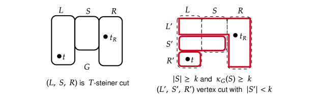
Let $G=(V,E)$ be a graph with terminal set $T\subseteq V$ . Let $(L,S,R)$ be a vertex cut in $G$ . We define the $k$ -left graph $G_{L}$ (w.r.t $(L,S,R)$ ) of $G$ as the graph $G$ after replacing $R$ with a clique $K_{R}$ of size $k$ (selecting an arbitrary set of $k$ vertices that contains one terminal denoted as $t_{R}$ ), followed by adding biclique edges between $S$ and $K_{R}$ . Optionally, we remove all edges inside $S$ , see Figure 1 for illustration. The definition of the $k$ -right graph $G_{R}$ is similar where $K_{L}$ is a clique replacing $L$ with $t_{L}$ as a terminal in $K_{L}$ .

Refer to caption — Figure 1: $G_{L},G_{R}$ are $k$ -left, $k$ -right graphs of $G$ w.r.t cut $(L,S,R)$ .

Let $G$ be a graph with terminal set $T$ . Let $(L,S,R)$ be a $T$ -Steiner cut, and let $T_{L}:=T\cap L$ , $T_{R}:=T\cap R$ . Let $G_{L}$ be the $k$ -left graph w.r.t. $(L,S,R)$ and denote $t_{R}$ to be an arbitrary terminal in the clique. We also define $G_{R}$ and $t_{L}$ symmetrically.

Lemma 3.7.

If $\kappa_{G}(T)<k$ , then $\min\{\kappa_{G}(S),\kappa_{G_{L}}(T_{L}\cup\{t_{R}\}),\kappa_{G_{R}}(T_{R}\cup\{t_{L}\})\}<k$ .

Proof.

If $|S|<k$ , then $\kappa_{G_{L}}(T_{L}\cup\{t_{R}\}),\kappa_{G_{R}}(T_{R}\cup\{t_{L}\})<k$ follows by Definition 3.6 and the fact that $(L,S,R)$ is a $T$ -Steiner cut as shown in the left side of Figure 2. Now we assume $|S|\geq k$ . Since $\kappa_{G}(T)<k$ , there is a min Steiner cut $(L^{\prime},S^{\prime},R^{\prime})$ of size less than $k$ . If $\kappa_{G}(S)<k$ , then we are done. Now assume $\kappa_{G}(S)\geq k$ . Thus, $S^{\prime}$ does not separate $x,y$ for all $x,y\in S$ . That is, $S\subseteq L^{\prime}\cup S^{\prime}$ or $S\subseteq S^{\prime}\cup R^{\prime}$ , i.e., $S\cap R^{\prime}=\emptyset$ or $S\cap L^{\prime}=\emptyset$ . WLOG, we assume $S\cap R^{\prime}=\emptyset$ . Since $S^{\prime}$ is a $T$ -Steiner cut, $R^{\prime}\cap T\neq\emptyset$ , and so there must be a terminal vertex from $T$ in $L\cap R^{\prime}$ or in $R\cap R^{\prime}$ . Let $t\in T$ be a terminal vertex in $L\cap R^{\prime}$ (otherwise, the argument is symmetric).

Next, we prove that $S^{\prime}\subseteq L\cup S$ (i.e., $S^{\prime}\cap R=\emptyset$ ) as shown in the right side of Figure 2. Let $Z:=N_{G}(L\cap R^{\prime})$ . Since $T\cap L^{\prime}\neq\emptyset$ and $t\in L\cap R^{\prime}$ , $Z$ is a $T$ -Steiner cut. Since $S\cap R^{\prime}=\emptyset$ and there is no edge from $L\cap R^{\prime}$ to $R$ as there are no edges from $L$ to $R$ , we have $Z=S^{\prime}\cap(L\cup S)\subseteq S^{\prime}$ . Therefore, $|S^{\prime}|=|S^{\prime}\cap(L\cup S)|+|S^{\prime}\cap R|=|Z|+|S^{\prime}\cap R|$ . Observe that $|S^{\prime}|=|Z|$ since $Z$ is a $T$ -Steiner cut where $Z\subseteq S^{\prime}$ and $S^{\prime}$ is a min $T$ -Steiner cut. So, $|S^{\prime}\cap R|=0$ , and thus $S^{\prime}\cap R=\emptyset$ .

Finally, we argue that $S^{\prime}$ is a $T_{L}\cup\{t_{R}\}$ -Steiner cut in $G_{L}$ , refer Figure 3. Since $R^{\prime}\cap S=\emptyset$ and $S^{\prime}\cap R=\emptyset$ , $S^{\prime}$ remains a separator in $G_{L}$ . It remains to prove that $S^{\prime}$ separates $t$ and $t_{R}$ in $G_{L}$ . Observe that $S^{\prime}$ separates $t$ and $y$ in $G$ for all $y\in R$ . In particular, $S^{\prime}$ separates $t$ and $t_{R}$ in $G$ . Therefore, $S^{\prime}$ separates $t$ and $t_{R}$ in $G_{L}$ . ∎

Lemma 3.8.

A separator of size less than $k$ in $G_{L}$ or $G_{R}$ is also a separator in $G$ . Furthermore, for all $x,y\in V(G_{L})$ (or in $V(G_{R})$ ), a min $(x,y)$ -separator of size less than $k$ in $G_{L}$ (or $G_{R}$ ) is also an $(x,y)$ -separator in $G$ .

Proof.

We prove for $G_{L}$ . The proof for $G_{R}$ is similar. Let $(L^{\prime},S,R^{\prime})$ be a vertex cut smaller than $k$ in $G_{L}$ . We prove that there is $S^{\prime\prime}\subseteq S^{\prime}$ such that $S^{\prime\prime}$ is a separator in $G$ . If true, then $S^{\prime}$ must also be a separator in $G$ , and we are done. Since $|S^{\prime}|<k$ and $K_{R}$ has $k$ vertices, there is a vertex $x\in K_{R}$ that is in $L^{\prime}$ or in $R^{\prime}$ . WLOG, $x\in L^{\prime}$ . Since we have biclique edges between $K_{R}$ and $S$ in $G_{L}$ and there is no edge between $L^{\prime}$ and $R^{\prime}$ , $S\subseteq L^{\prime}\cup S^{\prime}$ and $K_{R}\subseteq L^{\prime}\cup S^{\prime}$ .

By moving the clique to $L^{\prime}$ as shown in Figure 4, $(L^{\prime\prime},S^{\prime\prime},R^{\prime}):=(L^{\prime}\cup K_{R},S^{\prime}-K_{R},R^{\prime})$ is a vertex cut in $G_{L}$ . To obtain $G$ from $G_{L}$ , we replace $K_{R}$ with $R$ , add edges between $R$ and $R\cup S$ according to $G$ and (possibly) add edges inside $S$ . Since $K_{R}\subseteq L^{\prime\prime}$ and $S\subseteq L^{\prime\prime}\cup S^{\prime\prime}$ , we never add an edge from $L^{\prime\prime}\cup R$ to $R^{\prime}$ . Therefore, $(L^{\prime\prime}\cup R-K_{R},S^{\prime\prime},R^{\prime})$ is a vertex cut in $G$ , and so $S^{\prime\prime}=S^{\prime}-K_{R}\subseteq S^{\prime}$ remains a separator in $G$ . The proof for the second statement is similar. ∎

3.3 Terminal Reduction Algorithm

We now describe our algorithm that takes as inputs $G=(V,E),T\subseteq V$ and outputs either a separator of size less than $k$ or a terminal set $T^{\prime}\subset V$ of size $|T^{\prime}|<|T|/2$ such that $\kappa_{G}(T^{\prime})<k$ whenever $\kappa_{G}(T)<k$ . We only prove the correctness of Theorem 1.3 using this algorithm and defer the implementation and proof of runtime guarantee to the next section.

Algorithm.

Let $k,\phi,\bar{\phi}$ be the global parameters such that $\bar{\phi}>\phi$ . Given a graph $G$ , if it is a $(T,\phi)$ -expander, we can find mincut using Theorem 3.1 as any cut of size less than $k$ is $(T,k/\phi)$ -unbalanced. If $T$ has at most $10k/\phi$ terminals, we can run $(s,t)$ -max-flow on all pairs of terminals to find the mincut.

So we can assume that there are at least $10k/\phi$ many terminals, and the graph has $(T,\phi)$ -sparse cut. Let $(L,S,R)$ be a $(T,\bar{\phi})$ -sparse cut. We construct $G_{L}$ and $G_{R}$ w.r.t the vertex cut $(L,S,R)$ as defined in Definition 3.6 such that $t_{R}$ and $t_{L}$ are the terminals present in the clique $K_{R}$ and $K_{L}$ respectively and recurse on them. For $G_{L}$ , we consider the terminals present in $L$ and the terminal $t_{R}$ in $K_{R}$ i.e. $(T\cap L)\cup\{t_{R}\}$ , similarly, for $G_{R}$ . Note that we ignore the terminals of $S$ in both cases.

If either of the recursive calls returns a separator of size less than $k$ , we return that separator. Otherwise, they return terminal sets $S^{\prime}_{L}$ and $S^{\prime}_{R}$ such that $\kappa_{G_{L}}(S^{\prime}_{L})<k$ whenever $\kappa_{G_{L}}(T_{L}\cup\{t_{R}\})<k$ and $\kappa_{G_{R}}(S^{\prime}_{R})<k$ whenever $\kappa_{G_{R}}(T_{R}\cup\{t_{L}\})<k$ . From Lemma 3.7, we have $\min\{\kappa_{G}(S),\kappa_{G_{L}}(T_{L}\cup\{t_{R}\}),\kappa_{G_{R}}(T_{R}\cup\{t_{L}\})\}<k$ whenever $\kappa_{G}(T)<k$ . Hence we have $\min\{\kappa_{G}(S),\kappa_{G_{L}}(S^{\prime}_{L}),\kappa_{G_{R}}(S^{\prime}_{R})\}<k$ whenever $\kappa_{G}(T)<k$ and hence we return $T^{\prime}=S\cup S^{\prime}_{L}\cup S^{\prime}_{R}$ as the new terminal set.

We formally describe the algorithm in Algorithm 1 and prove its correctness in the following lemma.

Global variables: Connectivity parameter

k

and

0.5>\bar{\phi}>\phi>0

Input: A graph

G=(V,E)

and a terminal set

T\subseteq V

, and connectivity parameter

k

and

0.5>\bar{\phi}>\phi>0

Output: Either a separator of size less than

k

or a new terminal set

T^{\prime}\subseteq V

1 if $G$ is a $(T,\phi)$ -vertex expander or $|T|\leq 10k/\phi$ then

2 return

\emptyset

\kappa_{G}(T)\geq k

. Otherwise, return a separator of size less than

k

using all pairs max-flows or using Theorem 3.1.

3Let

(L,S,R)

be a

(T,\bar{\phi})

-sparse cut.

4 Let

G_{L}

and

G_{R}

k

-left and

k

-right graphs of

G

w.r.t.

(L,S,R)

5 Let

t_{R}

be a terminal in the clique of

G_{L}

, and

t_{L}

be a terminal in the clique of

G_{R}

6 Let

T_{L}=T\cap L

, and

T_{R}=T\cap R

S^{\prime}_{L}\leftarrow\textsc{ReduceTerminalSlow}_{k,\phi,\bar{\phi}}(G_{L},T_{L}\cup\{t_{R}\})

S^{\prime}_{R}\leftarrow\textsc{ReduceTerminalSlow}_{k,\phi,\bar{\phi}}(G_{R},T_{R}\cup\{t_{L}\})

9 if $S^{\prime}_{L}$ (or $S^{\prime}_{R}$ ) is a separator in $G_{L}$ (or $G_{R}$ ) of size $<k$ then

10 By Lemma 3.8, it must be a separator in

G

11 return the corresponding separator.

12else

S^{\prime}_{L}

and

S^{\prime}_{R}

are both new terminal sets of

G

14 return $S_{L}^{\prime}\cup S^{\prime}_{R}\cup S.$

Algorithm 1 ReduceTerminalSlow

{}_{k,\phi,\bar{\phi}}(G,T)

Lemma 3.9.

Algorithm 1 on $G,T$ with parameters $k,\phi,\bar{\phi}$ outputs either a separator of size $<k$ or a new terminal set $T^{\prime}\subseteq V$ such that $\kappa(T^{\prime})<k$ whenever $\kappa(T)<k$ .

Observe that the new terminal set $T^{\prime}$ size depends on the recursion depth, which we bound in the next section.

Proof.

We prove that Algorithm 1 outputs correctly as stated on every connected graph with a terminal set by induction on the number of terminals $t$ . Observe that the parameters $k,\phi,\bar{\phi}$ are fixed. When $t\leq 10k\phi^{-1}$ , it is the base case and we handle it by computing all pairs max-flow over the terminal set $T$ . Next, for all $t\geq 10k\phi^{-1}+1$ , we assume that the statement holds up to $t-1$ terminals, and we now prove that the statement continues to hold for $t$ terminals. If $G$ is a $(T,\phi)$ -expander, then we know that $G$ has a $(T,k/\phi)$ -unbalanced cut and we can use Theorem 3.1 in this case to detect a cut of size less than $k$ . Otherwise, let $(L,S,R)$ be a $(T,\bar{\phi})$ -sparse cut. Denote $T_{L}=T\cap L,T_{R}=T\cap R,T_{S}=T\cap S$ . We prove that $|T_{L}|,|T_{R}|\geq 2$ . If true, then $G_{L}$ and $G_{R}$ will have $|T_{L}\cup\{t_{R}\}|\leq t-1$ and $|T_{R}\cap\{t_{L}\}|\leq t-1$ terminals, respectively, so that we can apply inductive hypothesis on them. Suppose $|T_{L}|=1$ . Then, the expansion $h(L,S,R)=|S|/(1+|T_{S}|)$ . If $T_{S}=\emptyset$ , then $h(L,S,R)\geq 1>\bar{\phi}$ . Otherwise, $h(L,S,R)=\frac{|S|}{1+|T_{S}|}\geq\frac{|T_{S}|}{1+|T_{S}|}\geq 1/2>\bar{\phi}$ . In either case, we have a contradiction.

It remains to prove that Algorithm 1 on $G$ and terminal set $T$ outputs correctly as stated in the lemma. Let $S^{\prime}_{L}$ and $S^{\prime}_{R}$ be the output from $\textsc{ReduceTerminalSlow}_{k,\phi,\bar{\phi}}(G_{L},T_{L}\cup\{t_{R}\})$ and $\textsc{ReduceTerminalSlow}_{k,\phi,\bar{\phi}}(G_{R},T_{R}\cup\{t_{L}\})$ , respectively. By inductive hypothesis, $S^{\prime}_{L}$ is either a separator in $G_{L}$ of size $<k$ or a new terminal set such that $\kappa_{G_{L}}(S^{\prime}_{L})<k$ whenever $\kappa_{G}(T_{L}\cup\{t_{R}\})<k$ . Similarly, $S^{\prime}_{R}$ is either a separator in $G_{R}$ of size $<k$ or a new terminal set such that $\kappa_{G_{R}}(S^{\prime}_{R})<k$ whenever $\kappa_{G}(T_{R}\cup\{t_{L}\})<k$ . If $S^{\prime}_{L}$ or $S^{\prime}_{R}$ is a separator for $G_{L}$ or $G_{R}$ , respectively, then Lemma 3.8 implies that one of them is a separator in $G$ , and we are done. Now, assume that $S^{\prime}_{L}$ and $S^{\prime}_{R}$ are the new terminal sets. We prove that $\kappa_{G}(S^{\prime}_{L}\cup S^{\prime}_{R}\cup S)<k$ whenever $\kappa_{G}(T)<k$ . Let us assume that $\kappa_{G}(T)<k$ . We are done if $\kappa_{G}(S)<k$ . Now, assume $\kappa_{G}(S)\geq k$ . By Lemma 3.7, either $\kappa_{G_{L}}(T_{L}\cup\{t_{R}\})<k$ or $\kappa_{G_{R}}(T_{R}\cup\{t_{L}\})<k$ , and thus $\kappa_{G_{L}}(S^{\prime}_{L})<k$ or $\kappa_{G_{R}}(S^{\prime}_{R})<k$ . By Lemma 3.8, $\kappa_{G}(S^{\prime}_{L})<k$ or $\kappa_{G}(S^{\prime}_{R})<k$ , and we are done.∎

3.4 Fast Implementation of Algorithm 1

We have proved the correctness of Algorithm 1 (ReduceTerminalSlow) in the previous section. In this section, we use the following important lemma from [LS22] to implement ReduceTerminal following the approach in Algorithm 1.

Lemma 3.10 ([LS22]).

Let $G=(V,E)$ be an $n$ -vertex $m$ -edge graph with a terminal set $T\subseteq V$ . Given a parameter $0<\bar{\phi}\leq 1/10$ and $1\leq r\leq\left\lfloor\log_{20}n\right\rfloor$ , there is a deterministic algorithm, $\textsc{TerminalBalancedCutOrExpander}(G,T,\bar{\phi},r)$ , that computes a vertex cut $(L,S,R)$ (but possibly $L=S=\emptyset$ ) of $G$ (where we denote $T_{L\cup S}:=T\cap(L\cup S)$ and $T_{R\cup S}:=T\cap(R\cup S)$ ) such that $|S|\leq\bar{\phi}|T_{L\cup S}|$ which further satisfies

•

either $|T_{L\cup S}|,|T_{R\cup S}|\geq|T|/3$ ; or
•

$|T_{R\cup S}|\geq|T|/2$ and $G[R\cup S]$ is a $(T_{R\cup S},\phi)$ -vertex expander for some $\phi=\bar{\phi}/\log^{O(r^{5})}m$ .

The running time of this algorithm is $O(m^{1+o(1)+O(1/r)}\log^{O(r^{4})}(m)/\phi)$ .

Algorithm.

$\textsc{ReduceTerminal}_{k,\phi}$ takes $G=(V,E)$ and $T\subseteq V$ as inputs and outputs either a separator of size less than $k$ or a new terminal set of a smaller size where $k,\phi$ are the global parameters.

If the graph has a small number of terminals, say at most $10k/\phi$ , then we run max-flow on all pairs of the terminals, and we either return the mincut or return an empty terminal set denoting that $\kappa_{G}(T)\geq k$ . Let $r,\bar{\phi}$ be parameters as defined in the Algorithm 2 which are given as inputs to TerminalBalancedCutOrExpander along with $G,T$ that outputs a cut $(L,S,R)$ .

From the Lemma 3.10 guarantee, the graph $G$ is a $(T,\phi)$ -expander if $L=S=\emptyset$ . Based on the definition of the expander, there are at most $\Theta(k/\phi)$ number of terminals on the smaller side of the mincut; hence it is $(T,\beta)$ -unbalanced for $\beta=\Theta(k/\phi)$ and we use Theorem 3.1 (Unbalanced) to solve for a cut of size less than $k$ .

Hence, $L\neq S\neq\emptyset$ and we get a $(T,\bar{\phi})$ -sparse cut by Lemma 3.10. If $|S|<k$ , we return $S$ as the separator. Otherwise, we have the two cases mentioned in the Lemma 3.10. In both cases, we must recurse on the left side of the cut. Hence, we construct the $k$ -left graph $G_{L}$ as defined in Definition 3.6 and apply recursively $\textsc{ReduceTerminal}_{k,\phi}$ with $G_{L},(T\cap L)\cup\{t_{R}\}$ as inputs where $t_{R}$ is any arbitrary terminal in $R$ . If the output $S^{\prime}_{L}$ is a separator, then we return it.

Otherwise, we have to recurse on the right side, so we construct $G_{R}$ similarly. If we are in the first case of Lemma 3.10, then we simply call $\textsc{ReduceTerminal}_{k,\phi}$ with the terminal set $(T\cap R)\cup\{t_{L}\}$ , where $t_{L}$ is arbitrary terminal in $R$ . If the output $S^{\prime}_{R}$ is a separator, then we return it. Otherwise, $S^{\prime}_{R}$ is the terminal set that we need to recurse.

If we are in the second case of Lemma 3.10, then we have the guarantee that $G[S\cup R]$ is a $(T_{R\cup S},2\phi)$ -vertex expander. We prove that $k$ -right graph (w.r.t. $(L,S,R)$ ) $G_{R}$ is still an $(T_{R\cup S}\cup\{t_{L}\},\phi)$ -vertex expander. Note in this case we do not remove the edges inside $S$ while constructing $G_{R}$ .

Claim 3.11.

If $G[S\cup R]$ is a $(T_{R\cup S},2\phi)$ -vertex expander, then the $k$ -right graph $G_{R}$ is a $(T_{R\cup S}\cup\{t_{L}\},\phi)$ -vertex expander.

Proof.

Suppose there is a $(T_{R\cup S}\cup\{t_{L}\},\phi)$ -sparse cut $(L^{\prime},S^{\prime},R^{\prime})$ in $G_{R}$ . By removing the clique in $G_{R}$ , we obtain another cut $(L^{\prime\prime},S^{\prime\prime},R^{\prime\prime})$ in $G[S\cup R]$ where $L^{\prime\prime}=L^{\prime}-V(K_{L})$ $S^{\prime\prime}=S^{\prime}-V(K_{L})$ and $R^{\prime\prime}=R-V(K_{L})$ . The expansion $h(L^{\prime\prime},S^{\prime\prime},R^{\prime\prime})$ is

\frac{|S^{\prime\prime}|}{|T_{R\cup S}\cap(L^{\prime\prime}\cup S^{\prime\prime})|}\leq\frac{|S^{\prime}|}{|T_{R\cup S}\cap(L^{\prime}\cup S^{\prime})|}\leq\frac{|S^{\prime}|}{|(T_{R\cup S}\cup\{t_{L}\})\cap(L^{\prime}\cup S^{\prime})|-1}<2\phi.

The first inequality follows since $|T_{R\cup S}\cap(L^{\prime\prime}\cup S^{\prime\prime})|=|T_{R\cup S}\cap(L^{\prime}\cup S^{\prime})|$ . The last inequality follows since $(L^{\prime},S^{\prime},R^{\prime})$ is a $(T_{R\cup S}\cup\{t_{L}\},\phi)$ -sparse, and thus $|(T_{R\cup S}\cup\{t_{L}\})\cap(L^{\prime}\cup S^{\prime})|\geq 2$ . So, $(L^{\prime\prime},S^{\prime\prime},R^{\prime\prime})$ is $(T_{R\cup S},2\phi)$ -sparse in $G[S\cup R]$ , a contradiction. ∎

Hence, we can just use Unbalanced on $G_{R}$ with $(T\cap(R\cup S))\cup\{t_{L}\}$ as the terminal set and $\beta=\Theta(k/\phi)$ . If it returns a separator, we return it. Otherwise, we guarantee no terminal cut of size less than $k$ in $G_{R}$ ; hence, we need not recurse further so $S^{\prime}_{R}=\emptyset$ . Finally, we return the union of $S^{\prime}_{L},S,S^{\prime}_{R}$ as the new terminal set.

We describe the algorithm formally in Algorithm 2 and prove the correctness and running time guarantee in Lemma 3.12.

Global variables: the original input graph

G^{\textrm{orig}}=(V^{\textrm{orig}},E^{\textrm{orig}})

whose min degree is

\geq k

. The parameters

\phi=(1/\log^{(\log\log|V^{\textrm{orig}}|)^{6}}|E^{\textrm{orig}}|)\in(0,1/10)

and

k

are also global.

Input: A graph

G=(V,E)

with terminal set

T\subseteq V

Output: A separator of size

<k

or a new terminal set.

r\leftarrow\log\log|V|

\bar{\phi}\leftarrow 2\cdot\phi\cdot\log^{O(r^{5})}|E|

3 if $|T|\leq 10k/\phi$ then

4 Let

S^{\prime}

be a minimizer of

\min_{x,y\in T}\kappa_{G}(x,y)

5 return

S^{\prime}

|S^{\prime}|<k

, otherwise return an empty (terminal) set.

(L,S,R)\leftarrow\textsc{TerminalBalancedCutOrExpander}(G,\bar{\phi},r)

8 if $L=S=\emptyset$ then

S^{\prime}\leftarrow\textsc{Unbalanced}(G,T,\beta)

where

\beta=\Theta(k\phi^{-1})

using Theorem 3.1.

10 return

S^{\prime}

|S^{\prime}|<k

, otherwise return an empty (terminal) set.

12if $|S|<k$ then return $S$

Let

T_{L}=T\cap L,T_{L\cup S}=T\cap(L\cup S),T_{R}=T\cap R

and

T_{R\cup S}=T\cap(R\cup S)

// By Lemma 3.10,

(L,S,R)

(T,\bar{\phi})

-sparse.

13 Let

G_{L}

be the

k

-left graph of

G

w.r.t.

(L,S,R)

, and

t_{R}

be a terminal in the clique of

G_{L}

where we remove all edges in

E_{G_{L}}(S,S)

from

G_{L}

S^{\prime}_{L}\leftarrow\textsc{ReduceTerminal}_{\phi,k}(G_{L},T_{L}\cup\{t_{R}\})

16 if $S^{\prime}_{L}$ is a separator then

return $S^{\prime}_{L}$

|S^{\prime}_{R}|<k

19Let

G_{R}

be the

k

-right graph of

G

w.r.t.

(L,S,R)

, and

t_{L}

be a terminal in the clique of

G_{R}

where we remove all edges in

E_{G_{R}}(S,S)

from

G_{R}

if and only if

\min\{T_{L\cup S},T_{R\cup S}\}\geq|T|/3

21if $\min\{|T_{L\cup S}|,|T_{R\cup S}|\}\geq|T|/3$ then

S^{\prime}_{R}\leftarrow\textsc{ReduceTerminal}_{\phi,k}(G_{R},T_{R}\cup\{t_{L}\})

23 if $S^{\prime}_{R}$ is a separator then

return $S^{\prime}_{R}$

|S^{\prime}_{R}|<k

26else

27 By 3.11,

G_{R}

is a

(T_{R\cup S}\cup\{t_{L}\},\phi)

-vertex expander.

S^{\prime}_{R}\leftarrow\textsc{Unbalanced}(G_{R},T_{R\cup S}\cup\{t_{L}\},\beta)\text{ where }\beta=\Theta(k\phi^{-1})

using Theorem 3.1.

29 if $S^{\prime}_{R}$ is a separator of size $<k$ then

30 return $S^{\prime}_{R}$

31 else

S^{\prime}_{R}\leftarrow\emptyset

S^{\prime}_{L}

and

S^{\prime}_{R}

are new terminal sets.

34 return $S^{\prime}_{L}\cup S\cup S^{\prime}_{R}$ as a new terminal set.

Algorithm 2 ReduceTerminal

{}_{\phi,k}(G,T)

Lemma 3.12.

Let $G=(V,E)$ be a graph with a terminal set $T\subseteq V$ where $G$ has min-degree at least $k$ and $|V|=n,|E|=m,\phi\in(0,1/10)$ . The algorithm ReduceTerminal ${}_{\phi,k}(G,T)$ (Algorithm 2) either returns a separator of size $<k$ or a new terminal set $T^{\prime}\subseteq V$ such that $\kappa(T^{\prime})<k$ whenever $\kappa(T)<k$ . Furthermore, $|T^{\prime}|\leq\bar{\phi}|T|(1+\phi)^{O(\log n)}$ where $\bar{\phi}=\phi\cdot m^{o(1)}$ . The algorithm runs $O(m^{\prime 1+o(1)}\phi^{-1})$ time outside max-flow calls, and the total number of edges in all max-flow instances is $O(m^{\prime}k^{2}\phi^{-2}\log^{2}n)$ where $m^{\prime}=(1+4\bar{\phi})^{O(\log n)}m$ .

The main theorem Theorem 1.3 is implied by substituting an appropriate value of $\phi$ as given in Algorithm 2. The rest of the section is devoted to proving the Lemma 3.12.

Correctness.

We show that Algorithm 2 follows the description of Algorithm 1, i.e., it implements Algorithm 1. By Lemma 3.9, this means that Algorithm 2 outputs either a separator of size less than $k$ or a new terminal set $T^{\prime}\subseteq V$ such that $\kappa(T^{\prime})<k$ whenever $\kappa(T)<k$ . The base cases happen when $|T|\leq 10k/\phi$ (Algorithm 2) or when $L=S=\emptyset$ (Algorithm 2). The correctness is immediate if $|T|\leq 10k/\phi$ . If $L=S=\emptyset$ at Algorithm 2, then $G$ is a $(T,2\phi)$ -vertex expander, so $G$ contains a $(T,\beta)$ -unbalanced vertex mincut whenever $\kappa_{G}(T)<k$ . By Theorem 3.1, Unbalanced $(G,T,\beta)$ outputs a separator $S^{\prime}$ of size less than $k$ whenever $\kappa_{G}(T)<k$ . If $|S^{\prime}|\geq k$ , we have verified that $\kappa_{G}(T)\geq k$ , and thus an empty terminal set is returned correctly. If $|S|<k$ (Algorithm 2), then $S$ must be a separator of $G$ , and we are done.

We now assume that we do not execute the base cases. By Lemma 3.10, $(L,S,R)$ is a $(T,\bar{\phi})$ -sparse. We recurse on $(G_{L},T_{L}\cup\{t_{R}\})$ in the same way as in Algorithm 1. For $G_{R}$ , either we recurse on $(G_{R},T_{R}\cup\{t_{L}\})$ or we immediately solve $G_{R}$ . If $\min\{|T_{L\cup S}|,|T_{R\cup S}|\}\geq|T|/3$ , then we recurse on $(G_{R},T_{R}\cup\{t_{L}\})$ in the same way as in Algorithm 1. Otherwise, Lemma 3.10 together with 3.11 imply that $G_{R}$ is $(T_{R\cup S}\cup\{t_{L}\},\phi)$ -vertex expander. Thus, $G_{R}$ contains a $(T_{R\cup S}\cup\{t_{L}\},\beta)$ -unbalanced vertex mincut whenever $\kappa_{G_{R}}(T_{R\cup S}\cup\{t_{L}\})<k$ . By Theorem 3.1, Unbalanced $(G_{R},T_{R\cup S}\cup\{t_{L}\},\beta)$ (Algorithm 2) outputs a separator $S^{\prime}_{R}$ of size $<k$ whenever $\kappa_{G_{R}}(T_{R\cup S}\cup\{t_{L}\})<k$ . If $|S^{\prime}_{R}|\geq k$ , then $\kappa_{G_{R}}(T_{R\cup S}\cup\{T_{L}\})\geq k$ , and thus we can view the subproblem on $G_{R}$ as returning $S^{\prime}_{R}$ as an emptyset, and hence the new terminal set $S^{\prime}_{L}\cup S\cup S^{\prime}_{R}$ is returned according to Algorithm 1.

Recursion tree.

It remains to analyze the size of the new terminal and the total running time. We first set up notations regarding the recursion tree $\mathcal{T}$ . Let $G^{\textrm{orig}},T^{\textrm{orig}}$ be the graph and its terminal set at the root of the recursion tree $\textsc{ReduceTerminal}_{\phi,k}(G^{\text{orig}},T^{\text{orig}})$ . We represent each subproblem by $(G,T)$ , the graph and its terminal set. If $G$ is $(T,\phi)$ -vertex expander or $|T|\leq 10k/\phi$ , then we treat this subproblem as a leaf node in the recursion tree. Otherwise, we obtain a $(T,\bar{\phi})$ -sparse cut $(L,S,R)$ , and recurse on $(G_{L},T_{L}\cup\{t_{R}\})$ and $(G_{R},T_{R}\cup\{t_{R}\})$ . Here, we treat $(G_{L},T_{L}\cup\{t_{R}\})$ and $(G_{R},T_{R}\cup\{t_{L}\})$ as a left child and a right child – respectively of $(G,T)$ . Furthermore, for each internal node $(G,T)$ , we also denote $(G,T;(L,S,R))$ where $(L,S,R)$ is the sparse cut obtained in the subproblem. For the analysis, let us assume that Algorithm 2 is always false. Each subproblem’s sparse cut has size at least $k$ , which can only give a worse bound.

Lemma 3.13.

The depth of the recursion tree $\mathcal{T}$ is $O(\log|T^{\textrm{orig}}|)=O(\log n)$ .

Proof.

Let $(G,T)$ be any internal node in the recursion tree. Let $(L,S,R)$ be $(T,\bar{\phi})$ -sparse cut in $G$ with the properties as stated in Lemma 3.10. We show that the terminal set of each subproblem decreases by a constant factor. If $|T_{L\cup S}|,|T_{R\cup S}|\geq|T|/3$ , then $|T_{L}|,|T_{R}|\leq|T|-|T|/3\leq 2|T|/3$ . Therefore, $|T_{L}\cup\{t_{R}\}|,|T_{R}\cup\{t_{L}\}|\leq 2|T|/3+1\leq 0.77|T|$ . The last inequality follows since $|T|\geq 10k/\phi$ . Otherwise, $G_{R}$ is $(T_{R}\cup\{t_{L}\},\phi)$ -vertex expander, and we treat the right subproblem as a leaf in the recursion tree. In this case, $|T_{L}|=|T|-|T_{R\cup S}|\leq|T|/2$ , and thus $|T_{L}\cup\{t_{R}\}|=|T_{L}|+1\leq 0.6|T|$ . ∎

The size of the new terminal set.

If $\textsc{ReduceTerminal}_{\phi,k}(G^{\text{orig}},T^{\text{orig}})$ returns a separator, then it must be of size less than $k$ , and we are done. Now we assume that a terminal set $T^{\prime}$ is returned where we denote $t=|T^{\text{orig}}|,t^{\prime}=|T^{\prime}|$ . Thus, every subproblem in the recursion must return a (possibly empty) terminal set. Let $(G,T;(L,S,R))$ be an internal node in the recursion tree. Let $G_{L}$ and $G_{R}$ be the $k$ -left/-right graphs of $G$ w.r.t. $(L,S,R)$ , respectively. Denote $t_{0}=|T|$ , we have $|T_{L}\cup\{t_{R}\}|+|T_{R}\cup\{t_{L}\}|\leq t_{0}+2\leq(1+\phi)t_{0}$ . The last inequality follows since $|T|\geq 10k\phi^{-1}\geq 10\phi^{-1}$ for non-base cases. Therefore, at level, $i$ , the total number of terminals (as inputs) is at most $(1+\phi)^{i-1}t$ . Let $\ell$ be the recursion depth. The total number of terminals as inputs to each subproblem at all levels is $O((1+\phi)^{\ell+1}t)$ . Next, we bound the size of the output terminals. Observe that, every internal node $(G,T;(L,S,R))$ , $(L,S,R)$ is a $(T,\bar{\phi})$ -sparse cut, and thus $|S|\leq\bar{\phi}|T_{L\cup S}|\leq\bar{\phi}\cdot t_{0}$ . Therefore, the number of output terminals is at most $\bar{\phi}$ times the total number of input terminals. Thus, $|T^{\prime}|=t^{\prime}\leq\bar{\phi}(1+\phi)^{\ell+1}|T|\leq\bar{\phi}(1+\phi)^{O(\log n)}|T|$ . The last inequality follows by Lemma 3.13.

Running time.

We bound the total number of edges of the graphs (as an input to each subproblem) in the recursion tree. Let $(G,T;(L,S,R))$ be an internal node in the recursion tree. We assume that $\min\{T_{L\cup S},T_{R\cup S}\}\geq|T|/3$ because otherwise we would recurse only on $G_{L}$ . We denote $n_{0}=|V(G)|,m_{0}=|E(G)|,m_{L}=|E(G_{L})|,m_{R}=|E(G_{R})|$ . Therefore,

\displaystyle m_{L}+m_{R}\leq m_{0}+2(|S|k+k^{2})\leq m_{0}+4|S|k\leq m_{0}+4\bar{\phi}\cdot n_{0}k\leq m_{0}(1+4\bar{\phi})

The first inequality follows since there are $|S|k+k^{2}$ additional edges from biclique edges in $G_{L}$ and $G_{R}$ and the clique edges, and we remove edges between $S$ in both $G_{L}$ and $G_{R}$ . The second inequality follows since $|S|\geq k$ . The third inequality follows since $|S|\leq\bar{\phi}\cdot|T_{L\cup S}|\leq\bar{\phi}n_{0}$ . The last inequality follows since the min-degrees of $G_{L}$ and $G_{R}$ are at least $k$ .

Therefore, at level $i$ , the total number of edges is at most $O(m(1+4\bar{\phi})^{i-1})$ . By summing over all $i$ , the total number of edges in the recursion tree is $O(m(1+4\bar{\phi})^{\ell+1})=O(m(1+4\bar{\phi})^{O(\log n)})$ . Finally, we bound the running time using Theorem 3.1 at the base cases and Lemma 3.10 at each internal node of the recursion tree. At the base cases, every instance of $m^{\prime}$ edges takes $O(m^{\prime}\beta^{2}\log^{4}(n))=\tilde{O}(m^{\prime}k^{2}\phi^{-2})$ time outside the max-flows, and the number of edges in all max-flow instances is at most $O(m^{\prime}\beta^{2}\log^{5}(n))=O(m^{\prime}k^{2}\phi^{-2}\log^{5}(n))$ . At each internal node in the recursion, each instance of $m^{\prime}$ edges takes $m^{\prime 1+o(1)}\phi^{-1}$ .

4 A $(1+\epsilon)$ -Approximation Algorithm

In this section, we give a $(1+\epsilon)$ -approximation algorithm for vertex connectivity. Recall Theorem 1.2 from Section 1.

See 1.2

The main idea of the algorithm is to use two graphs³³3the first graph is an induced sub-graph of an expander and the second graph is small set vertex expander. and apply $(s,t)$ -min cut on all the edges of them. We start with defining the guarantees required from these graphs and then state and prove the correctness of the algorithm.

Lemma 4.1 (Induced sub-graph of Ramanujan expander).

Given an integer $n$ and a degree parameter $d$ , a graph $H=(V_{H},E_{H})$ with maximum degree $4d$ and $|V_{H}|=n$ can be constructed in time $O(nd)$ such that for any $L,R\subseteq V_{H}$ , if $|L|\cdot|R|\cdot d\geq 4c_{{\ref{lem:gabow00}}}^{2}n^{2}$ for universal constant $c_{{\ref{lem:gabow00}}}$ from Lemma 4.4, then $E_{H}(L,R)\neq\emptyset$ .

A graph $X=(V_{X},E_{X})$ is called $(\alpha,\beta)$ -vertex expander for some $\alpha\leq 1,\beta\geq 0$ , if for every subset $L\subset V_{X}$ with $|L|\leq\alpha|V_{X}|$ we have $|N_{X}(L)|\geq\beta|L|$ where $N_{X}(L)=\{u\in V\setminus L\mid\exists v\in L\text{ such that }(u,v)\in E_{X}\}$ represents the neighborhood of $L$ in $X$ .

Lemma 4.2 (Small set vertex expander).

Given an integer $n$ and a parameter $\epsilon$ , a $(\frac{\epsilon}{20c^{2}},\frac{2}{\epsilon})$ -vertex expander, $H=(V_{H},E_{H})$ with $|V_{H}|=n$ and maximum degree $O(1/\epsilon)$ can be constructed in $O(n/\epsilon)$ time.

Before proving Theorem 1.2, we must observe a structural property of the $(1+\epsilon)$ -approximate minimum cut. Let $\delta$ be the minimum degree of the graph $G$ .

Claim 4.3.

Let $(L,S,R)$ be any minimum vertex cut of size $\kappa_{G}$ in graph $G=(V,E)$ with minimum degree $\delta\geq(1+\epsilon)\kappa_{G}$ . We have $\min(|L|,|R|)\geq\epsilon\kappa_{G}$ .

Proof.

WLOG, we can assume $|L|\leq|R|$ and $v$ be any arbitrary vertex in $L$ . Since $(L,S,R)$ is a vertex cut, $N(v)\subseteq L\cup S\setminus\{v\}$ . So we have

(1+\epsilon)\kappa_{G}\leq\delta\leq|N(v)|\leq|L|+|S|-1=|L|+\kappa_{G}-1

which implies $|L|\geq\epsilon\kappa_{G}$ . ∎

The above lemma tells us that if the minimum degree of graph $\delta\geq(1+\epsilon)\kappa_{G}$ , every minimum cut has at least $\epsilon\kappa_{G}$ vertices on both sides. We are now ready to state our algorithm and prove its correctness and running time.

Input: A graph

G=(V,E)

, approximation parameter

\epsilon

Output: A separator

S

of graph

G

with guarantee of

|S|<\lfloor(1+\epsilon)\kappa_{G}\rfloor

1 Let

c_{{\ref{lem:gabow00}}}

be the universal constant given in Lemma 4.4.

2 Let

H_{1}=(V,E_{H_{1}})

be the graph constructed with

|V|,d=\frac{1600c_{{\ref{lem:gabow00}}}^{6}}{\epsilon^{2}}

as inputs to Lemma 4.1

3 Let

H_{2}=(V,E_{H_{2}})

be the

(\frac{\epsilon}{20c_{{\ref{lem:gabow00}}}^{2}},\frac{2}{\epsilon})

-vertex expander constructed with

|V|,\epsilon

as inputs to Lemma 4.2

4 Let

S

be the minimum separator seen so far, initialized with

V

5 for $e=(s,t)\in E_{H_{1}}\cup E_{H_{2}}$ do

6 Compute

T=

min

(s,t)

-separator in

G

7 if $|T|<|S|$ then

S=T

10if $\delta<|S|$ then

11 return

N(v)

where

v\in V

such that

\deg(v)=\delta

12else

13 return

S

Algorithm 3 ApproxVertexMinCut

(G,\epsilon)

We prove the correctness and running time of Algorithm 3, thus proving Theorem 1.2.

Proof of Theorem 1.2.

Let $(L,S,R)$ be a minimum vertex cut in the graph $G$ with $|V|=n$ . We construct $H_{1},H_{2}$ by giving required inputs to Lemmas 4.1 and 4.2 respectively. Since the three graphs $G,H_{1},H_{2}$ have same number of vertices, we can assume they are having same vertex set $V$ by mapping them arbitrarily.

If $|L|\geq\frac{\epsilon n}{20c_{{\ref{lem:gabow00}}}^{2}}$ and $|R|\geq\frac{\epsilon n}{20c_{{\ref{lem:gabow00}}}^{2}}$ , then in graph $H_{1}$ , we have

|L|\cdot|R|\cdot d\geq\frac{\epsilon n}{20c_{{\ref{lem:gabow00}}}^{2}}\cdot\frac{\epsilon n}{20c_{{\ref{lem:gabow00}}}^{2}}\cdot\frac{1600c_{{\ref{lem:gabow00}}}^{6}}{\epsilon^{2}}\geq 4c_{{\ref{lem:gabow00}}}^{2}n^{2}.

From the guarantee of Lemma 4.1 we have $E_{H_{1}}(L,R)\neq\emptyset$ hence, we find $S$ computing $(s,t)$ -separator across that edge.

Otherwise, we can assume WLOG $|L|<\frac{\epsilon n}{20c_{{\ref{lem:gabow00}}}^{2}}$ . We can also assume that $\delta\geq(1+\epsilon)\kappa_{G}$ otherwise, we would return the neighborhood of the minimum degree vertex in Algorithm 3. Hence from 4.3 we have $|L|\geq\epsilon\kappa_{G}$ .

From the guarantee of Lemma 4.2 we have, $|N_{H_{2}}(L)|\geq\frac{2}{\epsilon}|L|\geq 2\kappa_{G}$ . Hence, in $H_{2}$ there exists a neighbour of $L$ in $R$ as $|S|=\kappa_{G}$ , implies $E_{H_{2}}(L,R)\neq\emptyset$ . Applying $(s,t)$ -max-flow on two endpoints of an edge in $E_{H_{2}}(L,R)$ gives us the minimum separator.

We apply $(s,t)$ -max-flow on $G$ for every edge $(s,t)\in E_{H_{1}}\cup E_{H_{2}}$ which are at most $O(n/\epsilon^{2})$ in total. The total additional time to construct both $H_{1},H_{2}$ is at most $O(n/\epsilon^{2})$ from the time guarantees of Lemmas 4.1 and 4.2. ∎

The rest of the section discusses constructing the graphs $H_{1},H_{2}$ stated in Algorithm 3.

Induced sub-graph of Ramanujan expander.

Here we prove Lemma 4.1. We construct the first graph from Ramanujan expanders. Ramanujan expanders are graphs with the strongest spectral expansion guarantee, which by the expander mixing lemma (see e.g. [Vad12]), implies that any two large enough sub-sets have an edge between them. This is formally described in the following theorem taken from [Gab06].

Lemma 4.4 (Discussion above Lemma 2.4 in [Gab06]).

Given integers $n,d\in\mathbb{N}$ , there exists a $d^{\prime}$ -regular Ramanujan expander $X=(V_{X},E_{X})$ with $|V_{X}|\leq c_{{\ref{lem:gabow00}}}n$ , $d\leq d^{\prime}\leq 4d$ for some universal constant $c_{{\ref{lem:gabow00}}}$ and can be constructed in time $O(nd)$ . We also have guarantee that for any $L,R\subseteq V_{X}$ , if $|L|\cdot|R|\cdot d^{\prime}\geq 4|V_{X}|^{2}$ , then $E_{X}(L,R)\neq\emptyset$ .

Proof of Lemma 4.1.

Given integers $n,d$ apply Lemma 4.4 and construct $d^{\prime}$ -regular Ramanujan expander $X=(V_{X},E_{X})$ in time $O(nd)$ . We construct $H=(V_{H},E_{H})$ from $X$ as follows. Let $V_{H}$ be any arbitrary subset of $V_{X}$ of size $n$ and $E_{H}=E_{X}(V_{H},V_{H})$ which is the subset of edges $E_{X}$ whose both endpoints are in $V_{H}$ . Hence it takes at most $O(nd)$ total time to construct the graph $H$ . Maximum degree of $H$ is at most $d^{\prime}\leq 4d$ from Lemma 4.4.

For any $L,R\subseteq V_{H}\subseteq V_{X}$ , if we have

|L|\cdot|R|\cdot d^{\prime}\geq|L|\cdot|R|\cdot d\geq 4c_{{\ref{lem:gabow00}}}^{2}n^{2}\geq 4|V_{X}|^{2}

as $d^{\prime}\geq d$ , $|L||R|d\geq 4c_{{\ref{lem:gabow00}}}^{2}n^{2}$ and $|V_{X}|\leq c_{{\ref{lem:gabow00}}}n$ respectively. From Lemma 4.4 we have guarantee that $E_{X}(L,R)\neq\emptyset$ , hence $E_{H}(L,R)\neq\emptyset$ . ∎

Small set vertex expander.

Here we prove Lemma 4.2. As explained below, we create the second graph using Ramanujan expanders, which have a high spectral expansion that implies good vertex expansion.

Let $A$ be the adjacency matrix of the graph $G$ and $D$ be the diagonal matrix with $i^{th}$ diagnoral entry as $\deg(v_{i})$ where $v_{i}$ is the $i^{th}$ vertex of graph $G$ . Let $\lambda_{1}(G),\lambda_{2}(G),\dots$ be the eigenvalues of the matrix $AD^{-1}$ sorted from high to low according to their absolute values. We recall the following fact of Ramanujan graphs.

Fact 4.5 ([LPS86]).

Let $X=(V_{X},E_{X})$ be the $d^{\prime}$ -regular Ramanujan graph with $n^{\prime}$ vertices constructed using Lemma 4.4. We have $\lambda_{2}(X)\leq 2\sqrt{d^{\prime}-1}/d^{\prime}$ .

The spectral expansion $\gamma(G)$ of the graph $G$ is defined as $1-\lambda_{2}(G)$ . It is known that strong spectral expansion implies strong vertex expanders as stated below.

Lemma 4.6 (Lemma 4.6 from [Vad12] “spectral expansion implies vertex expansion”).

If $G$ is a regular digraph with spectral expansion $\gamma(G)=1-\lambda_{2}(G)$ then, for every $\alpha\in[0,1]$ , $G$ is an $(\alpha,\frac{1}{\alpha+(1-\alpha)\lambda_{2}(G)^{2}}-1)$ ⁴⁴4the lemma has extra $-1$ in the expansion parameter resulting due to change in the definition of $(\alpha,\beta)$ -vertex expander.-vertex expander.

Note that the statement works for undirected graphs by considering any undirected graph as a digraph by having two directed edges in both directions for each undirected edge. Now, we conclude the following claim.

Claim 4.7.

Given an integer $n$ and approximation parameter $\epsilon$ , we can construct a $(\frac{\epsilon}{10c_{{\ref{lem:gabow00}}}},\frac{4}{\epsilon})$ -vertex expander, $X=(V_{X},E_{X})$ of size at most $c_{{\ref{lem:gabow00}}}n$ and maximum degree $O(1/\epsilon)$ in time $O(n/\epsilon)$ .

Proof.

Let $X$ be the Ramanujan graph constructed with $n,d=40c_{{\ref{lem:gabow00}}}/\epsilon$ as inputs. From the guarantees of Lemma 4.4 we know that $|V_{X}|\leq c_{{\ref{lem:gabow00}}}n$ and is $d^{\prime}$ -regular with $d\leq d^{\prime}\leq 4d$ . From 4.5 we know that the second eigenvalue of $X$ , $\lambda_{2}(X)\leq 2\sqrt{d^{\prime}-1}/d^{\prime}\leq 2/\sqrt{d}$ .

Hence, by setting $\alpha=\epsilon/10c_{{\ref{lem:gabow00}}}$ in Lemma 4.6 we can conclude that $X$ is a $(\epsilon/10c_{{\ref{lem:gabow00}}},\beta)$ where $\beta=\frac{1}{(1-\alpha)\lambda_{2}(X)^{2}+\alpha}-1\geq\frac{1}{\frac{4}{d}+\frac{\epsilon}{10c_{{\ref{lem:gabow00}}}}}-1\geq\frac{4}{\epsilon}$ as $c_{{\ref{lem:gabow00}}}\geq 1$ and $\epsilon\leq 1$ . The time to construct the graph $X$ is at most $O(nd)=O(n/\epsilon)$ . ∎

Note that the graph $X$ we constructed above is of size at most $c_{{\ref{lem:gabow00}}}n$ , but we need a vertex expander of size $n$ . Taking any induced sub-graph of size $n$ would not solve the problem as it might not be a vertex expander. Below, we show that contracting groups of vertices where each group is small preserves the vertex expansion.

Claim 4.8.

If $G=(V_{G},E_{G})$ is a $(\alpha,\beta)$ -vertex expander with $|V_{G}|=\rho n,|E_{G}|=m$ for some parameter $\rho>1$ , then we can construct a $(\frac{\alpha}{\lceil\rho\rceil},\frac{\beta\lfloor\rho\rfloor}{\lceil\rho\rceil})$ -vertex expander $H=(V_{H},E_{H})$ of size $n$ in $O(m)$ time.

Proof.

If $\rho$ is an integer, we obtain $H$ by contracting arbitrary groups of $\rho$ vertices in $G$ . However, if $\rho$ is not an integer, we contract arbitrary groups of $\lfloor\rho\rfloor$ or $\lceil\rho\rceil$ many vertices together to achieve a graph of size exactly $n$ .

Let $L_{H}\subset V_{H}$ is of size at most $\alpha n/\lceil\rho\rceil$ . For each $v\in V_{H}$ let $C_{v}\subset V_{G}$ denote the set of vertices in $G$ contracted to form $v$ . Uncontracting the set of vertices in $L_{H}$ , we get $L_{G}=\cup_{v\in L_{H}}C_{v}$ . We have $|L_{G}|\leq\lceil\rho\rceil|L_{H}|\leq\alpha n$ , hence we have $|N_{G}(L_{G})|\geq\beta|L_{G}|$ as $G$ is a $(\alpha,\beta)$ -vertex expander.

Let $C[N_{G}(L_{G})]=\{v\in V_{H}\mid C_{v}\cap N_{G}(L_{G})\neq\emptyset\}$ be the set of contracted vertices in $V_{H}$ such that corresponding set $C_{v}\subset V_{G}$ has at least one vertex from $N_{G}(L_{G})$ . Observe that $C[N_{G}(L_{G})]=N_{H}(L_{H})$ . Every vertex in $C[N_{G}(L_{G})]$ has at least one edge from a vertex in $L_{H}$ as the edge across $L_{G}$ and $N_{G}(L_{G})$ is preserved after contraction. Hence, $C[N_{G}(L_{G})]\subseteq N_{H}(L_{H})$ . Every vertex $v\in N_{H}(L_{H})$ has a vertex $u\in L_{H}$ such that $(u,v)\in E_{H}$ . Uncontracting $u,v$ we have every vertex $w\in C_{v}$ that has edges from some vertex $x\in C_{u}\subset L_{G}$ should belong to $N_{G}(L_{G})$ , hence $v\in C[N_{G}(L_{G})]$ and we have $N_{H}(L_{H})\subseteq C[N_{G}(L_{G})]$ .

We have

|N_{H}(L_{H})|=|C[N_{G}(L_{G})]|\geq\frac{|N_{G}(L_{G})|}{\lceil\rho\rceil}\geq\frac{\beta|L_{G}|}{\lceil\rho\rceil}\geq\frac{\beta\lfloor\rho\rfloor}{\lceil\rho\rceil}|L|.

The first and third inequalities follow as we contract at most $\lceil\rho\rceil$ and at least $\lfloor\rho\rfloor$ many vertices in $G$ to construct $H$ . Hence, expansion is at least $\frac{\beta\lfloor\rho\rfloor}{\lceil\rho\rceil}$ .

The time taken to contract arbitrary vertices is at most $O(m)$ by just going over each edge and mapping them to the new contracted vertices. ∎

We now conclude the proof of Lemma 4.2.

Proof of Lemma 4.2.

With $n,\epsilon$ as inputs to 4.7, we construct a $(\frac{\epsilon}{10c_{{\ref{lem:gabow00}}}},\frac{4}{\epsilon})$ -vertex expander of size $\rho n$ where $1\leq\rho\leq c_{{\ref{lem:gabow00}}}$ in time $O(n/\epsilon)$ with $O(n/\epsilon)$ edges. We now use 4.8 to reduce the size of the graph and construct a $(\frac{\epsilon}{10c_{{\ref{lem:gabow00}}}\lceil\rho\rceil},\frac{4\lfloor\rho\rfloor}{\epsilon\lceil\rho\rceil})$ -vertex expander in time $O(n/\epsilon)$ , which is also a $(\frac{\epsilon}{20c_{{\ref{lem:gabow00}}}^{2}},\frac{2}{\epsilon})$ -vertex expander as $c_{{\ref{lem:gabow00}}}\geq 1$ . Hence, the total time is at most $O(n/\epsilon)$ . ∎

5 Open Problems

Exact vertex connectivity.

It remains elusive whether there exists a linear-time deterministic algorithm for vertex connectivity as postulated by [AHU74]. Even an algorithm with running time $\widehat{O}(mn)$ , independent from $k$ , is already very interesting as asked by Gabow [Gab06]. The currently fastest deterministic algorithm can be obtained by plugging an almost-linear-time max flow algorithm by [BCG⁺23] into the algorithm by Gabow [Gab06]. This will result in an algorithm that takes $\widehat{O}(m(n+k\min\{k,\sqrt{n}\})=\widehat{O}(mn^{1.5})$ time.

Approximate vertex connectivity.

Can we obtain an $(1+\epsilon)$ -approximation algorithm using $o(n)$ max-flow calls? The problem seems challenging to us even when we promise that there exists a vertex mincut $(L,S,R)$ where $|L|,|S|,|R|=\Omega(n)$ . Note that if randomization is allowed in this case, we can solve the problem with high probability by sampling $O(\log n)$ vertex pairs $(s,t)$ and compute $(s,t)$ vertex mincut, taking a total time of only $O(\log n)$ max flow calls.

Steiner vertex connectivity.

Our terminal reduction algorithm (Theorem 1.3) does not guarantee that $T^{\prime}\subset T$ , i.e., the output terminal is a subset of the input terminal. Is it possible to strengthen our algorithm to guarantee this with the same running time? This would imply a deterministic $\widehat{O}(mk^{2})$ -time algorithm for the Steiner vertex mincut problem, matching the conditional lower bound for dense graphs [HLSW23]. A randomized algorithm for Steiner vertex mincut with near-optimal $\widehat{O}(mk^{2})$ time is implicit in the literature.⁵⁵5To see this, let $T$ be the terminal set and $(L,S,R)$ be a Steiner vertex mincut of size less than $k$ . The algorithm starts by sampling each terminal with probability $1/k$ and so, with probability $\Omega(1/k^{2})$ , we have $T\cap S$ is empty, but both $T\cap L$ and $T\cap R$ are not empty. Assuming this event, one can use the isolating vertex cut technique together with further subsampling (see [LNP⁺21]) to detect a Steiner mincut using $\log^{O(1)}n$ max-flows. By repeating the algorithm $O(k^{2}\log n)$ times, we will detect a Steiner mincut with high probability.

Acknowledgement

This project has received funding from the European Research Council (ERC) under the European Union’s Horizon 2020 research and innovation programme under grant agreement No 759557.

References

[AHU74] Alfred V. Aho, John E. Hopcroft, and Jeffrey D. Ullman. The Design and Analysis of Computer Algorithms. Addison-Wesley, 1974.
[BCG⁺23] Jan van den Brand, Li Chen, Maximilian Probst Gutenberg, Rasmus Kyng, Yang P. Liu, Richard Peng, Sushant Sachdeva, and Aaron Sidford. A deterministic almost-linear time algorithm for minimum-cost flow. In FOCS, 2023.
[BDD⁺82] Michael Becker, W. Degenhardt, Jürgen Doenhardt, Stefan Hertel, Gerd Kaninke, W. Kerber, Kurt Mehlhorn, Stefan Näher, Hans Rohnert, and Thomas Winter. A probabilistic algorithm for vertex connectivity of graphs. Inf. Process. Lett., 15(3):135–136, 1982.
[CGK14] Keren Censor-Hillel, Mohsen Ghaffari, and Fabian Kuhn. Distributed connectivity decomposition. In PODC, pages 156–165. ACM, 2014.
[CKL⁺22] Li Chen, Rasmus Kyng, Yang P. Liu, Richard Peng, Maximilian Probst Gutenberg, and Sushant Sachdeva. Maximum flow and minimum-cost flow in almost-linear time. In FOCS, pages 612–623. IEEE, 2022.
[CR94] Joseph Cheriyan and John H. Reif. Directed s-t numberings, rubber bands, and testing digraph k-vertex connectivity. Combinatorica, 14(4):435–451, 1994. Announced at SODA’92.
[CT91] Joseph Cheriyan and Ramakrishna Thurimella. Algorithms for parallel k-vertex connectivity and sparse certificates (extended abstract). In STOC, pages 391–401. ACM, 1991.
[EH84] Abdol-Hossein Esfahanian and S. Louis Hakimi. On computing the connectivities of graphs and digraphs. Networks, 14(2):355–366, 1984.
[ET75] Shimon Even and Robert Endre Tarjan. Network flow and testing graph connectivity. SIAM J. Comput., 4(4):507–518, 1975.
[Eve75] Shimon Even. An algorithm for determining whether the connectivity of a graph is at least k. SIAM J. Comput., 4(3):393–396, 1975.
[FNS⁺20] Sebastian Forster, Danupon Nanongkai, Thatchaphol Saranurak, Liu Yang, and Sorrachai Yingchareonthawornchai. Computing and testing small connectivity in near-linear time and queries via fast local cut algorithms. In SODA, pages 2046–2065. SIAM, 2020.
[Gab06] Harold N. Gabow. Using expander graphs to find vertex connectivity. J. ACM, 53(5):800–844, 2006. Announced at FOCS’00.
[Gal80] Zvi Galil. Finding the vertex connectivity of graphs. SIAM J. Comput., 9(1):197–199, 1980.
[Hen97] Monika Rauch Henzinger. A static 2-approximation algorithm for vertex connectivity and incremental approximation algorithms for edge and vertex connectivity. J. Algorithms, 24(1):194–220, 1997.
[HLSW23] Zhiyi Huang, Yaowei Long, Thatchaphol Saranurak, and Benyu Wang. Tight conditional lower bounds for vertex connectivity problems. In STOC, pages 1384–1395. ACM, 2023.
[HRG00] Monika Rauch Henzinger, Satish Rao, and Harold N. Gabow. Computing vertex connectivity: New bounds from old techniques. J. Algorithms, 34(2):222–250, 2000. Announced at FOCS’96.
[HRW17] Monika Henzinger, Satish Rao, and Di Wang. Local flow partitioning for faster edge connectivity. In Proceedings of the Twenty-Eighth Annual ACM-SIAM Symposium on Discrete Algorithms, SODA 2017, Barcelona, Spain, Hotel Porta Fira, January 16-19, pages 1919–1938, 2017.
[HT73] John E. Hopcroft and Robert Endre Tarjan. Dividing a graph into triconnected components. SIAM J. Comput., 2(3):135–158, 1973.
[Kar00] David R. Karger. Minimum cuts in near-linear time. J. ACM, 47(1):46–76, 2000. announced at STOC’96.
[Kle69] D Kleitman. Methods for investigating connectivity of large graphs. IEEE Transactions on Circuit Theory, 16(2):232–233, 1969.
[KP20] Karthik Cs and Merav Parter. Deterministic replacement path covering. CoRR, abs/2008.05421, 2020.
[KT15] Ken-ichi Kawarabayashi and Mikkel Thorup. Deterministic global minimum cut of a simple graph in near-linear time. In STOC, pages 665–674. ACM, 2015.
[Li21] Jason Li. Deterministic mincut in almost-linear time. In STOC, pages 384–395. ACM, 2021.
[LLW88] Nathan Linial, László Lovász, and Avi Wigderson. Rubber bands, convex embeddings and graph connectivity. Combinatorica, 8(1):91–102, 1988. Announced at FOCS’86.
[LNP⁺21] Jason Li, Danupon Nanongkai, Debmalya Panigrahi, Thatchaphol Saranurak, and Sorrachai Yingchareonthawornchai. Vertex connectivity in poly-logarithmic max-flows. In STOC ’21: 53rd Annual ACM SIGACT Symposium on Theory of Computing, Virtual Event, Italy, June 21-25, 2021, pages 317–329. ACM, 2021.
[LP02] H. W. Lenstra and Carl Pomerance. Primality testing with gaussian periods. In Manindra Agrawal and Anil Seth, editors, FST TCS 2002: Foundations of Software Technology and Theoretical Computer Science, pages 1–1, Berlin, Heidelberg, 2002. Springer Berlin Heidelberg.
[LP20] Jason Li and Debmalya Panigrahi. Deterministic min-cut in poly-logarithmic max-flows. In 61st IEEE Annual Symposium on Foundations of Computer Science, FOCS 2020. IEEE Computer Society, 2020.
[LPS86] A Lubotzky, R Phillips, and P Sarnak. Explicit expanders and the ramanujan conjectures. In Proceedings of the Eighteenth Annual ACM Symposium on Theory of Computing, STOC ’86, page 240–246, 1986.
[LS22] Yaowei Long and Thatchaphol Saranurak. Near-optimal deterministic vertex-failure connectivity oracles. In 63rd IEEE Annual Symposium on Foundations of Computer Science, FOCS 2022, Denver, CO, USA, October 31 - November 3, 2022, pages 1002–1010. IEEE, 2022.
[Mat87] David W. Matula. Determining edge connectivity in o(nm). In FOCS, pages 249–251. IEEE Computer Society, 1987.
[Men27] Karl Menger. Zur allgemeinen kurventheorie. Fund. Math., 10:(1):96––115, 1927.
[NI92] Hiroshi Nagamochi and Toshihide Ibaraki. A linear-time algorithm for finding a sparse k-connected spanning subgraph of a k-connected graph. Algorithmica, 7(5&6):583–596, 1992.
[NSY19] Danupon Nanongkai, Thatchaphol Saranurak, and Sorrachai Yingchareonthawornchai. Breaking quadratic time for small vertex connectivity and an approximation scheme. In STOC, pages 241–252. ACM, 2019.
[Pod73] VD Podderyugin. An algorithm for finding the edge connectivity of graphs. Vopr. Kibern, 2:136, 1973.
[SY22] Thatchaphol Saranurak and Sorrachai Yingchareonthawornchai. Deterministic small vertex connectivity in almost linear time. In FOCS, pages 789–800. IEEE, 2022.
[Tar72] Robert Endre Tarjan. Depth-first search and linear graph algorithms. SIAM J. Comput., 1(2):146–160, 1972. Announced at FOCS’71.
[Vad12] Salil P. Vadhan. Pseudorandomness. Now Publishers Inc., Hanover, MA, USA, 2012.

Deterministic kk-Vertex Connectivity in k2k^{2} Max-flows

Abstract

1 Introduction

1.1 Our Results

Theorem 1.1.

Theorem 1.2.

1.2 Techniques

Theorem 1.3 (Terminal reduction).

Proof of Theorem 1.1.

Terminal Reduction Framework.

Handling Terminal-unbalanced Vertex Cuts.

Using Ramanujan graphs for Approximate Mincuts.

1.3 Organization

2 Preliminaries

3 An Exact Algorithm

3.1 Unbalanced Vertex Cuts

Theorem 3.1.

Lemma 3.2.

Lemma 3.3 (Lemma 4.2 of [LNP+21]).

Proof of Theorem 3.1.

Definition 3.4 (Hit and Miss hash family).

Claim 3.5.

Proof.

Proof of Lemma 3.2.

3.2 Terminal Cut Recursion Lemma

Definition 3.6.

Lemma 3.7.

Proof.

Lemma 3.8.

Proof.

3.3 Terminal Reduction Algorithm

Algorithm.

Lemma 3.9.

Proof.

3.4 Fast Implementation of Algorithm 1

Lemma 3.10 ([LS22]).

Algorithm.

Claim 3.11.

Proof.

Lemma 3.12.

Correctness.

Recursion tree.

Lemma 3.13.

Proof.

The size of the new terminal set.

Running time.

4 A (1+ϵ)(1+\epsilon)-Approximation Algorithm

Lemma 4.1 (Induced sub-graph of Ramanujan expander).

Lemma 4.2 (Small set vertex expander).

Claim 4.3.

Proof.

Proof of Theorem 1.2.

Induced sub-graph of Ramanujan expander.

Lemma 4.4 (Discussion above Lemma 2.4 in [Gab06]).

Proof of Lemma 4.1.

Small set vertex expander.

Fact 4.5 ([LPS86]).

Lemma 4.6 (Lemma 4.6 from [Vad12] “spectral expansion implies vertex expansion”).

Claim 4.7.

Proof.

Claim 4.8.

Proof.

Proof of Lemma 4.2.

5 Open Problems

Exact vertex connectivity.

Approximate vertex connectivity.

Steiner vertex connectivity.

Acknowledgement

References

Deterministic $k$ -Vertex Connectivity in $k^{2}$ Max-flows

Lemma 3.3 (Lemma 4.2 of [LNP⁺21]).

4 A $(1+\epsilon)$ -Approximation Algorithm