Detecting parity violation from axion inflation with third generation detectors
Abstract
A gravitational wave background is expected to emerge from the superposition of numerous gravitational wave sources of both astrophysical and cosmological origin. A number of cosmological models can have a parity violation, resulting in the generation of circularly polarised gravitational waves. We investigate the constraining power of third generation Einstein Telescope and Cosmic Explorer detectors, for a gravitational wave background generated by early universe axion inflation.
Introduction— A stochastic gravitational wave background (SGWB) is expected to be created from the overlap of gravitational waves (GWs) coming from many independent sources. A number of early universe cosmological sources leading to a SGWB have been proposed, including inflation Chung et al (2000), cosmic strings Vilenkin et al (2000), first order phase transitions (see, e.g. Caprini et al (2016); Hindmarsh et al (2020)), or cosmological models inspired from string theory (see, e.g. Gasperini (1993); Gasperini 2 (2007)).
A number of mechanisms in the early universe can create parity violation Alexander et al (2006) that may manifest itself in the production of asymmetric amounts of right- and left-handed circularly polarised isotropic GWs. A detection and subsequent analysis of a polarised SGWB can place constraints on parity violating theories. Searches for parity violation in the LIGO-Virgo data has been explored Crowder et al (2006); Martinovic et al (2006).
In this study we focus on parity violation effects from axion inflation sourced GWs (e.g., Sorbo (2011); Neil Barnaby and Marco Peloso (2011); Mohamed M. Anber and Lorenzo Sorbo (2012)) in the context of the upcoming 3rd generation (3g) detectors Einstein Telescope (ET) ET_Collab (2021) and Cosmic Explorer (CE) Reitze et al (2006).
We adopt the formalism Martinovic et al (2006) presented in Naoki Sto and Atsushi Taruya (2012). We first highlight the methodology and then apply it to a parity violating axion inflation model.
Method— We perform parameter estimation and fit GW models to data using a hybrid frequentist-Bayesian approach Andrew Matas and Joseph Romano (2020). We construct a Gaussian log-likelihood for a multi-baseline network
| (1) |
is the frequency-dependent cross-correlation estimator of the SGWB for detectors , and its variance Bruce Allen and Joseph Romano (1999) for model parameters . The cross-correlation statistics are constructed using strain data from the individual detectors. We assume that correlated noise sources have been either filtered out Michael W. Coughlin (2018) or accounted for Meyers et al. (2020). The normalised GW energy density model we fit to the data is
| (2) |
stands for the standard overlap reduction function of detectors , and denote the overlap function associated with the parity violation term Joseph D. Romano and Neil J. Cornish (2017). The polarisation degree, , takes on values between -1 (fully left polarisation) and 1 (fully right polarisation), with for unpolarised isotropic SGWB. [More details can be seen in Appendix A.]
Axion Inflation— Consider a pseudoscalar inflaton field coupled to U(1) gauge fields as Michael S. Turner and Lawrence M. Widrow (1988); Garretson, W. Daniel and Field, George B. and Carroll, Sean M. (1992); Anber, Mohamed M and Sorbo, Lorenzo (2006)
| (3) |
() is the (dual) field strength tensor, is the mass scale suppressing higher dimensional operators of the theory, and parametrises the strength of the inflaton gauge field coupling, for all . The resulting equations of motion imply
| (4) |
where is defined as
| (5) |
stands for the potential of the inflaton field, is the number of e-folds, we have partial derivatives and , and dot denotes a derivative with respect to cosmic time . Equation (4), obtained under the assumption , , , can be then used to numerically calculate the evolution of in terms of frequency as Domcke, Valerie and Pieroni, Mauro and Binétruy, Pierre (2016)
| (6) |
Domcke, Valerie and Pieroni, Mauro and Binétruy, Pierre (2016) and defined as the total number of e-folds after the CMB scales exited the horizon. In terms of the number of e-folds, can be written as .
Given a scalar potential , one can use Planck 2018 data Aghanim, N. et al. (2020) to impose parameter constraints. A well-approximated solution for tensor and scalar perturbations reads Neil Barnaby and Marco Peloso (2011); Linde, Andrei and Mooij, Sander and Pajer, Enrico (2013)
| (7) |
and
| (8) |
with
being the radiation energy density today and the reduced Planck mass set to unity.
There is an additional constraint one however should take into account. Density perturbations produced during inflation could collapse and form primordial black holes (PBHs), leading to a possible risk of PBH overproduction Josan, Amandeep S. and Green, Anne M. and Malik, Karim A. (2009); Byrnes, Christian T. and Copeland, Edmund J. and Green, Anne M. (2012); Linde, Andrei and Mooij, Sander and Pajer, Enrico (2013). The upper bound on scalar power spectrum from the non-detection of PBHs is García-Bellido, Juan and Peloso, Marco and Unal, Caner (2016).
Among the different axion inflation models, let us consider the well-motivated quadratic model A.D. Linde (1983); Makino, Nobuyoshi and Sasaki, Misao (1991); McAllister, Liam and Silverstein, Eva and Westphal, Alexander (2010); Dimopoulos, S and Kachru, S and McGreevy, J and Wacker, J G (2008)
| (9) |
from the chaotic potential class A.D. Linde (1983). Resulting spectra with maximum strength () Domcke, Valerie and Pieroni, Mauro and Binétruy, Pierre (2016) and gauge fields are shown in Fig. 1.
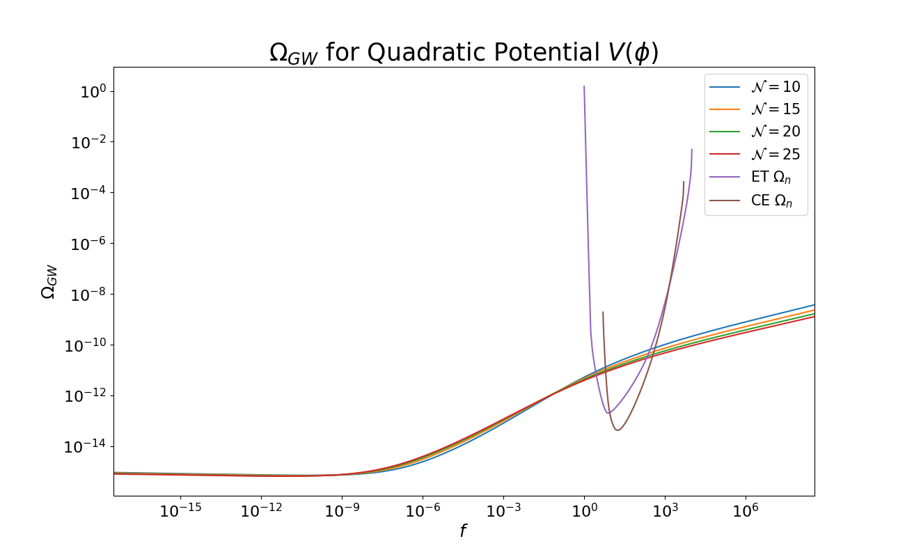
The corresponding polarisation degree reads Sorbo (2011):
| (10) |
We show in Fig. 2 the polarisation degree for GW spectra with and .
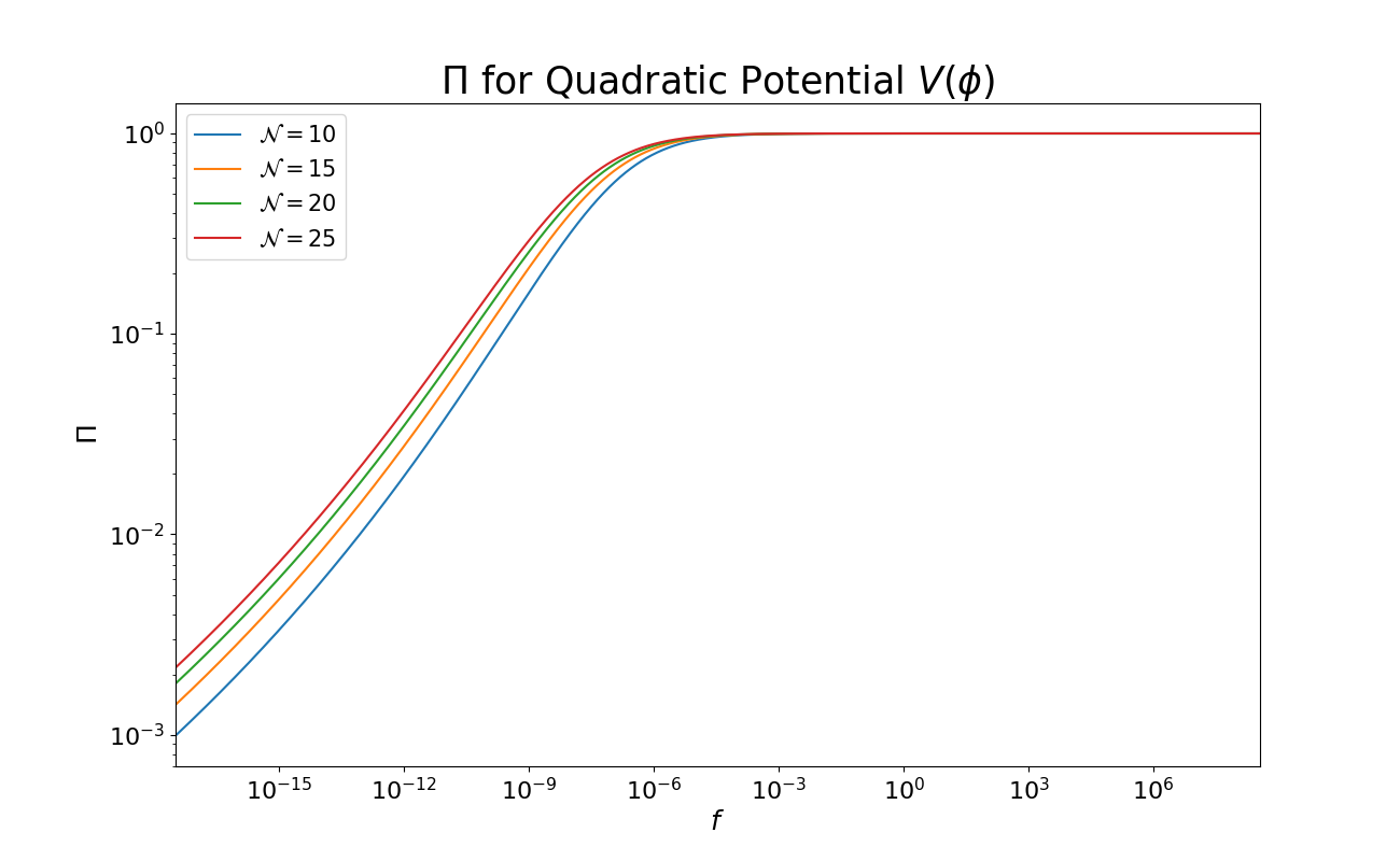
For Hz, almost entirely right-handed polarisation (approximately constant ) is expected, as one can see from Fig. 2.
Analysing a LIGO and Virgo network with A+ noise sensitivity design Barsotti, L., McCuller, L., Evans, M., Fritschel, P.The A+ design curve we have found that such a configuration could not provide any promising results, hence we will consider a 3g network.
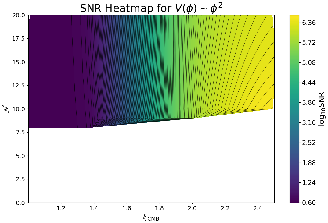
Results— Using ET and CE noise sensitivity curves Evans, M., Sturani, R., Vitale, S., Hall, E.Unofficial sensitivity curves (ASD), we construct a combined noise energy density Joseph D. Romano and Neil J. Cornish (2017). For the quadratic model we are focusing on, we consider 3500 random samples of discrete number of gauge fields , assuming also . For these samples we then calculate the corresponding spectra using Eqs. (7) and (8). If the resulting is below the PBH upper limit, we compute the corresponding signal-to-noise (SNR) ratio assuming years of observation Joseph D. Romano and Neil J. Cornish (2017). Our results, shown in Fig. 3, imply that quadratic models with and yield strong GW spectra with (all below the PBH upper limit).
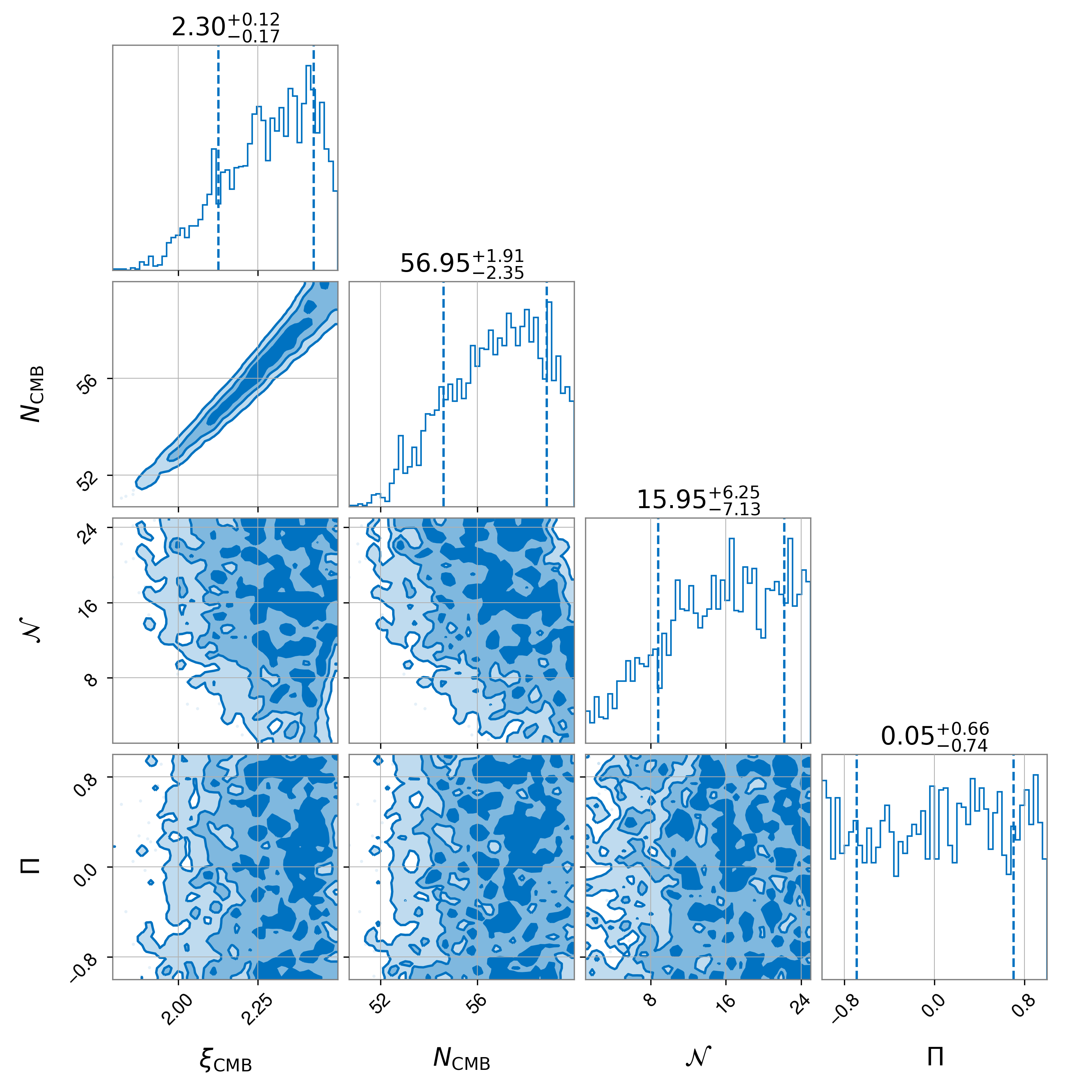
Let us first consider a triangular, three interferometer (60 degree opening angles, each separated by 10 km) design for the ET network located at the Virgo detector site. We inject a GW signal assuming an observation time of 3 years, , and . We search uniformly for , number of U(1) gauge fields , total e-folds and parity violation parameter . The corner plot of the posterior distribution is shown in Fig. 4. It is clear that while reasonable constraints can be placed on and , this is not the case for . Poor constraints on are expected since different values of lead to similar spectra within the relevant ET frequency range (see Fig. 1). An inability to place constraints on is also clear since for the ET network, two ET interferometers have resulting in for any value of when using this formalism. The Bayes factor clearly indicates a preference for the quadratic model with respect to noise.
To improve the parameter estimation, let us add additional 3g detectors. As one can see from Fig. 3, a large SNR could be obtained with and . We thus perform 500 Monte Carlo GW injections with , assuming and . The choice of is made such that we have the strongest signal (see, Fig. 1). We analyse our results using one ET located at the Virgo site, with either one Cosmic Explorer (CE) located at the LIGO Hanford detector site Aasi, J. and others (2015), or two CEs located at the LIGO Hanford and Livingston sites, respectively.
In Fig. 5 we plot the percent confidence that based off of each injection’s results 111Percent confidence that is the proportion of the posterior distribution that is greater than 0.. We list in Table 1 the injected for which 68%, 95% and 99.7% confidence can be achieved.
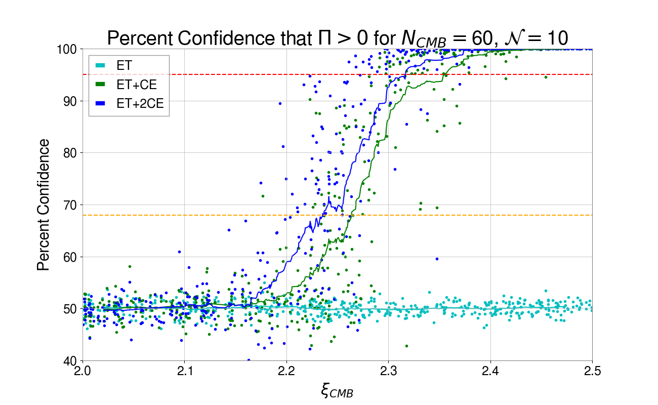
| Confidence | ET + CE | ET + 2 CEs |
|---|---|---|
| 68% | 2.26 | 2.24 |
| 95% | 2.35 | 2.32 |
| 99.7% | 2.43 | 2.39 |
Figure 5 clearly shows that additional 3g detectors improve our parity violation detection outlook. For quadratic models with , one can claim with at least 95% certainty using just two 3g detectors.
We plot in Fig. 6 the Bayes factors for the 500 injections. It is clear that the strength of improves drastically with each additional CE detector in the network. Strong preference () for our parity violating quadratic potential model can be achieved with .
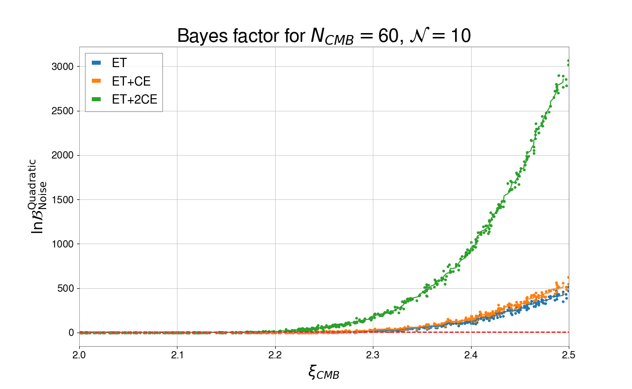
It is worth noting that our analysis assumed a total number of e-folds . A smaller would generate stronger in the 3g detector frequency range. Thus, our results must be seen as a conservative insight for the quadratic potential model.
Conclusions— We have studied detection of parity violation with 3g detectors sourced from axion inflation focusing on the quadratic potential.
Using this model, we showed that we can avoid the overproduction of PBHs by considering at least 10 U(1) gauge field couplings. Large SNR was obtained when .
We showed that a SGWB with large examined by a ET network alone can constrain and reasonably well, but it is unable to constrain the polarisation degree of the spectrum . Despite this, a Bayes factor was obtained in this analysis - indicating a strong preference for the quadratic axion inflation model with respect to noise.
Adding additional CE detectors to the network, we can better constrain the polarisation degree. With two 3g detectors (ET and CE) alone, one can claim with at least 95% confidence that when . However, a network of three 3g detectors (ET and 2 CEs) is needed in order to make a confident claim about the detection of a quadratic axion inflation signature. Each additional CE detector added to the 3g network results in a drastic improvement in retrieved .
Acknowledgements.
We thank LIGO-Virgo-KAGRA collaboration stochastic members for discussions related to axion inflation. We acknowledge computational resources provided by the LIGO Laboratory and supported by National Science Foundation Grants PHY-0757058 and PHY-0823459. This paper has been given LIGO DCC number LIGO-P2100430, an Einstein Telescope (ET) documentation number ET-0457A-21, and a KCL TPPC number 2021-93. M.S. is supported in part by the Science and Technology Facility Council (STFC), United Kingdom, under the research grant ST/P000258/1. Software packages used in this paper are matplotlib mat (2007), numpy np (2011), bilby bilby (2019), ChainConsumer cs (2016).Appendix A Methods
We normalize GW energy density for our data with
| (11) |
using model parameters , where we denote as the standard overlap reduction function of two detectors , and as the overlap function associated with the parity violation term defined as:
| (12) |
where stands for the contraction of the tensor modes of polarisation to the detector’s geometry. The polarisation degree, , takes on values between -1 (fully left polarisation) and 1 (fully right polarisation), with being an unpolarised isotropic SGWB.
To proceed we perform parameter estimation and fit GW models to data using a hybrid frequentist-Bayesian approach Andrew Matas and Joseph Romano (2020). We construct a Gaussian log-likelihood for a multi-baseline network
| (13) |
where is the frequency-dependent cross-correlation estimator of the SGWB for detectors , and is its variance Bruce Allen and Joseph Romano (1999). We assume that correlated noise sources have been either filtered out Michael W. Coughlin (2018) or accounted for Meyers et al. (2020). The normalised GW energy density model we fit to the data is , with parameters including both GW parameters as well as parameters of the model.
References
- Chung et al (2000) Daniel J.H. Chung, Edward W. Kolb, Antonio Riotto and Igor I. Tkachev, Physical Review D 62, (2000), URL http://dx.doi.org/10.1103/PhysRevD.62.043508.
- Vilenkin et al (2000) A. Vilenkin, and T. Damour, Physical Review Letters 85, 3761–3764 (2000), URL http://dx.doi.org/10.1103/PhysRevLett.85.3761.
- Caprini et al (2016) C. Caprini, M. Hindmarsh, T. Konstandin, J. Kozaczuk, G. Nardini, J.M. No, A. Petiteau, P. Schwaller and G. Servant, et al. JCAP 04, 601 (2016), URL https://doi.org/10.1088/1475-7516/2016/04/001.
- Hindmarsh et al (2020) M. Hindmarsh M. Lüben, J. Lumma and M. Pauly, SciPostPhysLectNotes.24 (2020), URL https://doi.org/10.21468/SciPostPhysLectNotes.24.
- Gasperini (1993) M. Gasperini, and G. Veneziano, Astroparticle Physics 1, 317–339 (1993), URL http://dx.doi.org/10.1016/0927-6505(93)90017-8.
- Gasperini 2 (2007) M. Gasperini, Elements of String Cosmology (2007).
- Alexander et al (2006) S. Alexander, M. Peskin, M. Sheikh-Jabbari, Physical Review Letters 96, (2006), URL http://dx.doi.org/10.1103/PhysRevLett.96.081301.
- Crowder et al (2006) S.G. Crowder, R. Nambda, V. Mandic, S. Mukohyama, M. Peloso, Physical Letters B 726, (2013), URL http://dx.doi.org/10.1016/j.physletb.2013.08.077.
- Martinovic et al (2006) K. Martinovic, C. Badger, M. Sakellariadou, V. Mandic, Physical Letters D 104, (2021), URL http://dx.doi.org/10.1103/PhysRevD.104.L081101.
- Sorbo (2011) L. Sorbo, Journal of Cosmology and Astroparticle Physics 2011, (2011), URL http://dx.doi.org/10.1088/1475-7516/2011/06/003.
- Neil Barnaby and Marco Peloso (2011) N. Barnaby, M. Peloso, Physical Review Letters 106, (2011), URL http://dx.doi.org/10.1103/PhysRevLett.106.181301.
- Mohamed M. Anber and Lorenzo Sorbo (2012) M.M. Anber, L. Sorbo, Physical Review D 85, (2012), URL http://dx.doi.org/10.1103/PhysRevD.85.123537.
- ET_Collab (2021) ET collaboration, URL http://www.et-gw.eu.
- Reitze et al (2006) D. Reitze, R. Adhikari, S. Ballmer, B. Barish, L. Barsotti, G. Billingsley, D.A. Brown, Y. Chen, D. Coyne, R. Eisenstein, M. Evans, P. Fritschel, E. Hall, A. Lazzarini, G. Lovelace, J. Read, B.S. Sathyaprakash, D. Shoemaker, J. Smith, C. Torrie, S. Vitale, R. Weiss, C. Wipf, M. Zucker, URL https://arxiv.org/abs/1907.04833.
- Naoki Sto and Atsushi Taruya (2012) N. Seto, T. Atsushi, Phys. Rev. Lett. 99, (2007), URL https://link.aps.org/doi/10.1103/PhysRevLett.99.121101.
- Andrew Matas and Joseph Romano (2020) A. Matas, J. Romano, Physical Review D 103, (2021), URL https://link.aps.org/doi/10.1103/PhysRevD.103.062003.
- Bruce Allen and Joseph Romano (1999) B. Allen, J. Romano, Physical Review D 59, (1999), URL https://link.aps.org/doi/10.1103/PhysRevD.59.102001.
- Michael W. Coughlin (2018) M.W. Coughlin et al., Physical Review D 97, (2018), URL https://link.aps.org/doi/10.1103/PhysRevD.97.102007.
- Meyers et al. (2020) P.M. Meyers, K. Martinovic, N. Christensen, M. Sakellariadou, Physical Review D 102, (2020), URL https://link.aps.org/doi/10.1103/PhysRevD.102.102005.
- Joseph D. Romano and Neil J. Cornish (2017) J. Romano, N.J. Cornish, Living Reviews in Relativity 20, (2017), URL http://dx.doi.org/10.1007/s41114-017-0004-1.
- Michael S. Turner and Lawrence M. Widrow (1988) M.S. Turner, L.M. Widrow, Phys. Rev. D 37, (1988), URL https://link.aps.org/doi/10.1103/PhysRevD.37.2743.
- Garretson, W. Daniel and Field, George B. and Carroll, Sean M. (1992) W.D. Garretson, G.B. Field, S.M. Carroll, Phys. Rev. D 46, (1992), URL http://dx.doi.org/10.1103/PhysRevD.46.5346.
- Anber, Mohamed M and Sorbo, Lorenzo (2006) M.M. Anber, L. Sorbo, Journal of Cosmology and Astroparticle Physics 2006, (2006), URL http://dx.doi.org/10.1088/1475-7516/2006/10/018.
- Domcke, Valerie and Pieroni, Mauro and Binétruy, Pierre (2016) V. Domcke, M. Pieroni, P. Binétruy, Journal of Cosmology and Astroparticle Physics 2016, (2016), URL http://dx.doi.org/10.1088/1475-7516/2016/06/031.
- Aghanim, N. et al. (2020) N. Aghanim et al., Astronomy & Astrophysics 641, (2020), URL http://dx.doi.org/10.1051/0004-6361/201833910.
- Linde, Andrei and Mooij, Sander and Pajer, Enrico (2013) A. Linde, S. Mooij, E. Enrico, Physical Review D 87, (2013), URL http://dx.doi.org/10.1103/PhysRevD.87.103506.
- Josan, Amandeep S. and Green, Anne M. and Malik, Karim A. (2009) A.S. Josan, A.M. Green, K.A. Malik, Physical Review D 79, (2009), URL http://dx.doi.org/10.1103/PhysRevD.79.103520.
- Byrnes, Christian T. and Copeland, Edmund J. and Green, Anne M. (2012) C.T. Byrnes, E.J. Copeland, A.M. Green, Physical Review D 86, (2012), URL http://dx.doi.org/10.1103/PhysRevD.86.043512.
- García-Bellido, Juan and Peloso, Marco and Unal, Caner (2016) J. García-Bellido, M. Peloso, C. Unal, Journal of Cosmology and Astroparticle Physics 2016, (2016), URL http://dx.doi.org/10.1088/1475-7516/2016/12/031.
- A.D. Linde (1983) A.D. Linde, Physics Letters B 129, (1983), URL https://www.sciencedirect.com/science/article/pii/0370269383908377.
- Makino, Nobuyoshi and Sasaki, Misao (1991) N. Makino, M. Sasaki, Progress of Theoretical Physics 86, (1991), URL https://doi.org/10.1143/ptp/86.1.103.
- McAllister, Liam and Silverstein, Eva and Westphal, Alexander (2010) L. McAllister, E. Silverstein, A. Westphal, Physical Review D 82, (2010), URL http://dx.doi.org/10.1103/PhysRevD.82.046003.
- Dimopoulos, S and Kachru, S and McGreevy, J and Wacker, J G (2008) S. Dimopoulos, S. Kachru, J. McGreevy, J. Wacker, Journal of Cosmology and Astroparticle Physics 2008, (2008), URL http://dx.doi.org/10.1088/1475-7516/2008/08/003.
- (34) L. Barsotti, L. McCuller, M. Evans, P. Fritschel, URL https://dcc.ligo.org/LIGO-T1800042/public.
- Evans, M., Sturani, R., Vitale, S., Hall, E.Unofficial sensitivity curves (ASD) M. Evans, R. Sturani, S. Vitale, E. Hall, URL https://dcc.ligo.org/LIGO-T1500293/public.
- Aasi, J. and others (2015) J. Aasi et al., Class. Quant. Grav. 32, (2015), URL http://dx.doi.org/10.1088/0264-9381/32/7/074001.
- mat (2007) J.D. Hunter, Computing in Science & Engineering 9, 90–95 (2007), URL https://link.aps.org/doi/10.1109/MCSE.2007.55.
- np (2011) S. van der Walt, S.C. Colbert, and G. Varoquaux, Computing in Science & Engineering 13, 22–30 (2011).
- bilby (2019) G. Ashton et al, Astrophys. J. Suppl. 241, 27 (2019), URL https://link.aps.org/doi/10.3847/1538-4365/ab06fc.
- cs (2016) S.R. Hinton, The Journal of Open Source Software 1, 00045 (2016), URL https://link.aps.org/doi/10.21105/joss.00045.