Detecting ionized bubbles around luminous sources during the reionization era using HI 21-cm signal
Abstract
Measuring the properties of the intergalactic medium (IGM) and sources during the Epoch of Reionization (EoR) is of immense importance. We explore the prospects of probing the IGM and sources through redshifted 21-cm observations of individual ionized bubbles surrounding known luminous sources during the EoR. Accordingly, we simulate HI 21-cm maps, foreground contaminants, and system noise which are specific to the uGMRT and SKA1-Low observations. Following the subtraction of the foreground from the total visibility, we employ a visibility-based matched filter technique to optimally combine the desired HI 21-cm signal while minimizing the system noise. Our analysis suggests that these ionized bubbles can be detected with more than significance using approximately and hours of observation time with the uGMRT at redshift and , respectively, when the mean neutral hydrogen fraction outside the targeted bubble is . The SKA1-Low should be able to detect these bubbles with more than significance using only hrs of observations. The total observing time increases both for the uGMRT and SKA1-Low when the mean neutral hydrogen fraction outside the targeted bubble decreases. Further, we investigate the impact of foreground subtraction on the detectability and find the signal-to-noise ratio decreases when smaller bandwidth is used. More importantly, we show that the matched filtering method can measure ionized bubble radius and constrain HI-neutral fraction reasonably well, providing deeper insights into the source properties and the intergalactic medium.
1 Introduction
It is widely accepted that ionizing UV radiation from the first galaxies and quasars began to ionize the neutral hydrogen (HI) in the intergalactic medium (IGM) during the redshift range from to [1, 2, 3, 4]. During this process, fully ionized regions, commonly referred to as ionized bubbles, began to form around these early galaxies and quasars, marking the onset of the epoch of reionization (EoR). As time progressed, these ionized bubbles grew and eventually merged, resulting in the ionization of the entire universe [5, 6, 7].
In recent times, there have been detections of several bright QSOs during the EoR [8, 9, 10, 11, 12, 13, 14, 15], and a handful of bright galaxies have also been detected at high redshifts as well [16, 17]. These bright, luminous sources will produce large ionized bubbles (HII regions) around them within the IGM. At the initial and intermediate stages of reionization, isolated or nearly isolated ionized bubbles are expected, which will remain buried inside the neutral (or partially ionized) IGM. Observations of redshifted HI 21-cm signal are a promising tool to study the epoch of reionization, including the individual ionized regions [18, 19, 20, 21, 22, 23, 24, 25, 26]. However, there are enormous challenges associated with these detections, as the signal is weaker by several orders of magnitude compared to the foreground contaminants [27, 28, 29, 30]. Moreover, the system noise is much stronger than the desired HI signal.
Previous studies have explored the detection of HII regions in HI 21-cm images [31, 18, 32, 23, 24, 25, 26]. This method enables direct estimation of the HI neutral fraction, the sizes of ionized bubbles, and the properties of the underlying sources. However, direct imaging of HI using redshifted 21-cm signal during the Epoch of Reionization (EoR) is challenging with current instruments like the uGMRT, LOFAR, MWA due to their limited sensitivities. The SKA1-Low is anticipated to produce images of individual ionized bubbles using the HI 21-cm signal, but this requires considerably long observation times.
This work investigates the prospects of individually detecting isolated ionized bubbles within the IGM, around known luminous sources using the matched filter algorithm. This technique works when the system noise of the radio interferometer dominates over the targeted HI signal. But the functional form of the targeted signal is known. The idea of applying a matched filter technique was first proposed in [33], which presents a visibility-based analytical framework to study the feasibility of detecting individual ionized bubbles during the EoR through radio-interferometric observations of redshifted HI 21-cm radiation. Later, it was shown that fluctuating intergalactic medium outside the targeted ionized bubble behaves as noise and hinders the detection of ionized bubbles of small sizes with radius Mpc [34]. Subsequent work such as [35] used detailed numerical simulations to study the detection prospects and associated challenges. [36] presents scaling relations, which enable us to quickly estimate detection prospects for various ionized bubble sizes, redshifts, and instruments. Further, [37] used a Bayesian framework to explore the possibility of constraining the parameters that characterize the bubbles. This approach of detecting individual ionized bubbles in HI 21-cm maps is complementary to the widely followed approach of detecting the summary statistics of the signal such as the power spectrum, bispectrum, etc. While the statistical methods probe the large scale behavior of the reionizing sources and the intergalactic medium [38, 39, 40, 41, 42, 43, 44], our approach sheds light on individual sources, ionized regions, and surrounding neutral medium. Interpreting the detection is also straightforward in our approach, unlike the statistical methods which might be complicated and model-dependent.
The majority of previous investigations have primarily focused on modeling HI 21-cm signal around ionized bubbles. In this work, we focus on targeted detection i.e., the location of the central luminous source is known from other observations. Along with simulated HI 21-cm maps which have a known source, we also simulate foreground contaminants and system noise. This is something that was not explicitly included in the previous works. Furthermore, we generated mock visibilities at baselines typical of the uGMRT/SKA1-Low observations. After subtracting the foreground from the total mock signal, we employ the matched filter technique on the residual signal. In that sense, the procedure adopted in this work resembles more with real observations. Moreover, we examine the constraints that observations with the uGMRT and SKA1-Low can impose on measuring bubble sizes and ionization fractions.
The outline of the paper is as follows: Section 2 provides a brief overview of the basics of the HI 21-cm signal around ionized bubbles. In section 3, we explain our methods to simulate the HI 21-cm signal around ionized bubbles, foreground contaminants, the generation of visibilities at baselines specific to a particular experiment, and system noise. Section 4 discusses foreground subtraction from the total visibilities and the application of the matched filter technique. Our results are presented in Section 5, while Section 6 presents a summary of the work undertaken in the paper alongside a discussion. Throughout our analysis we use the cosmological parameters , , , , and consistent with the WMAP measurements [45].
2 The HI 21-cm signal
During the EoR, the ionizing radiation from the first generation of luminous sources, such as galaxies and quasars, leads to the emergence of HII regions (ionized bubbles) around these sources, and the remaining neutral (HI) medium surrounds these ionized regions. The surrounding HI medium is expected to emit a line emission with a rest-frame wavelength of approximately cm, which arises due to the hyperfine spin-flip transition in the neutral hydrogen atoms. This redshifted HI 21-cm signal emitted from these surrounding HI mediums can be observed as a differential brightness temperature against the Cosmic Microwave Background, and one can express this differential brightness temperature as [46],
| (2.1) |
, , and are the HI spin temperature, CMB temperature, and the optical depth for the HI 21-cm line emission respectively. All these quantities depend on redshift and the line of sight direction . Under the assumption that the HI 21-cm optical depth is small enough () during the EoR, the above equation can be written as [47],
| (2.2) |
and are the mass density of neutral hydrogen and the average mass density of total hydrogen (neutral and ionized). and are the matter and baryon density parameter, is the dimensionless Hubble parameter and is the Hubble parameter at redshift respectively. The term inside the square brackets arises due to the redshift space distortion, and is the divergence of the peculiar velocity along the line of sight. Since the HI spin temperature of the neutral hydrogen in the IGM is expected to be coupled to the kinetic temperature of the gas during the EoR via the Lyman- coupling [48, 49, 50], it is expected to be much higher than the temperature of CMB (). Therefore, one can usually neglect the term (1 - ) in the HI 21-cm differential brightness temperature expression during the EoR. It is easily seen that the differential brightness temperature of the HI 21-cm signal directly probes the neutral hydrogen content () in the IGM. In the absence of neutral hydrogen in the HII regions, this differential brightness temperature is expected to be zero. Therefore, this allows us to probe the individual ionized bubbles within the neutral IGM.
In this paper, we specifically focus on individual HII regions around high redshift bright quasars and galaxies like the ones reported in [8] and [17], located at redshift and respectively. We expect large HII regions extending up to several tens of comoving Mpc around those bright luminous sources [8, 17]. Our ultimate objective is to investigate the detectability of such individual ionized regions using radio interferometric observations of HI 21-cm signal. The following section presents mock simulations of similar ionized bubbles around very bright quasars and galaxies during the EoR.
3 Simulating mock data
To investigate the prospects of detecting ionized bubbles individually in HI 21-cm maps, we first simulate mock data that resembles the uGMRT and SKA1-Low observations and at observational frequencies relevant to the EoR. It consists of simulations of the HII region around bright quasars/galaxies in large-scale HI maps, foreground contaminants, and system noise from radio interferometers. Subsequently, these simulated maps are converted into visibilities that mimic the uGMRT/SKA1-Low-like observations.
Our simulations are centered around two different observing frequencies, MHz and MHz, corresponding to the redshifts of and , respectively, for the HI 21-cm line emission. The selection of these two frequencies is motivated by the discoveries of a bright QSO at redshift [8] and a large ionized bubble at redshift [17]. The angular size of our simulation cube is set to which is closer to the uGMRT/SKA1-Low primary field of view at the observing frequencies considered here. Our simulation box has a total of grids on each side with a resolution of Mpc and a total comoving length of Mpc on each side. This results in an angular resolution of and a total angular size of . Here, we have used up to frequency channels with a total bandwidth of MHz, resulting in a channel width of kHz.
3.1 HI 21-cm signal around ionized bubbles
Here, we briefly describe simulated ionized regions surrounding a very bright quasar at , and around a collection of galaxies at during the EoR. First, we simulated the dark-matter distribution using the -body code222https://github.com/rajeshmondal18/N-body developed by [51]. We simulated this within a cubic box of the comoving size of Mpc with grids and the same number of particles. The minimum halo mass resolved in this simulation is , corresponding to a minimum of dark matter particles, each with a mass of . We note that our simulations do not include the contributions of low-mass halos in the range to . In reality, these halos are expected to play a significant role in the reionization of the IGM, potentially giving rise to more diffuse, complex, and smaller ionized structures during the EoR. Then we use a Friends-of-Friends 333https://github.com/rajeshmondal18/FoF-Halo-finder (FoF) [52] halo finder to identify the collapsed halos that host the galaxies/bright quasars. These galaxies/quasars serve as the sources of ionizing photons during the EoR. Subsequently, the resolution of simulated cubes is degraded to grids. This resolution resembles the corresponding angular resolution of the uGMRT and SKA1-Low and has the added benefit of reduced computational requirements for simulation. We then employ a semi-numerical prescription [53, 54, 55] on these outputs to simulate ionization maps and the HI 21-cm differential brightness temperature maps.
The semi-numerical approach compares the average number of ionizing photons and neutral hydrogen atoms within a spherical region of radius around a grid cell. If the ionization condition is met for any radius , then the grid cell is reckoned to be ionized, within that region. Otherwise, an ionized fraction value of is assigned to that grid cell. This procedure is repeated for varying radius up to a maximum value , over the whole simulation box. It is assumed that the number of ionizing photons from halos, contributed to the ionization of the IGM, follows the relation , where is the mass of the corresponding halo.
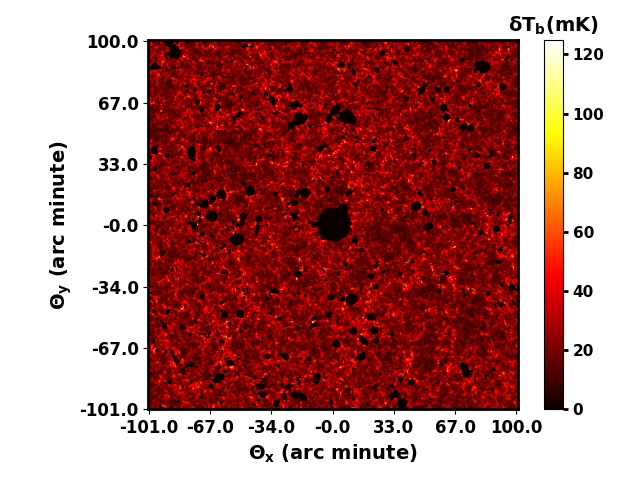
Here, we consider two scenarios. First, we aim to simulate an ionized region around a very bright quasar at a redshift of similar to the one reported in [8]. In the second case, we simulate an ionized region around a collection of galaxies at redshift as reported in [17]. In the first scenario, we assume that such a very bright quasar is hosted by the most massive halo (of mass found in our simulation [20]. We further assume that the ionizing photon emission rate by the QSO is [35, 20]. We note that along with the central quasar, many galaxies reside in and outside the QSO ionized regions. These galaxies are also contributing ionizing photons. The mass-averaged neutral Hydrogen fraction resulting from galaxies outside the QSO HII region is at a redshift of . In figure 1 (top left panel), the resulting HI 21cm map is shown with the ionized bubble around the quasar in the center of the map. The ionized region around the central bright QSO is considerably bigger (of radius around comoving Mpc) than all other ionized regions produced by the galaxies.
In the second case, we consider a collection of galaxies near the most massive halo (of mass ) in our simulation at . Simulation specifications such as the cubic box size, total number of particles used, and number of grids along a direction are the same as above. The ionizing luminosity of these galaxies, including the most massive halo in our simulation, is adjusted to create an HII bubble with a radius of Mpc, and the resulting mass-averaged neutral fraction is around . The ionized bubble from this scenario is shown in the top right panel of figure 1. We see that the ionized bubble in this scenario is slightly aspherical in shape, mainly because it is created by a collection of sources located at different locations inside the bubble.
In the above two cases, the targeted HII bubbles are isolated and nearly spherical. This geometry arises because the ionizing radiation from other sources is negligible, and the IGM outside the targeted bubbles remains highly neutral. While these scenarios may be suitable at the onset of reionization, they are likely unrealistic for the later stages of the process. At later stages of reionization, ionized bubbles around very bright sources are surrounded by neighboring ionized regions, leading to an aspherical shape for the targeted bubble. The third scenario accounts for this complexity. The bottom panel of Fig. 1 displays a 2D map of the differential brightness temperature () at redshift , where the central targeted HII bubble appears highly aspherical. The quasar at the center is the same as the first case. Surrounding it there are numerous other HII regions, unlike the first case. This results in a much lower mean neutral fraction, which is in this scenario.
We want to mention the considerable uncertainty regarding the ionizing photon emissivity rate from QSO, and therefore, the photon emissivity rate and the resulting QSO HII region may vary. The consequences of this uncertainty will be discussed later in the paper.


3.2 Foreground simulations
The astrophysical foregrounds that contaminate the EoR HI 21-cm signal observations comprise various components [56], including diffuse galactic synchrotron emission, radio synchrotron emission from point-like sources, free-free radio emission from diffuse ionized gas, etc.
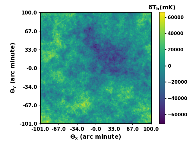
The diffuse galactic synchrotron emission (DSGE) is one of the most dominant foreground components. We model the angular power spectrum corresponding to the diffuse galactic synchrotron emission using a power-law formulation [57] as,
| (3.1) |
Here, MHz and . The power-law index, , is set to , and the amplitude is based on previous work [58]. The parameter describes how the power spectrum changes with frequency, which is set to [29, 30]. This simplified model allows us to simulate DGSE maps and to study their impact on the detection of individual ionized bubbles in the HI 21-cm maps. We use the following equation to generate Fourier components of the DGSE on each gridded baseline , which is given by
| (3.2) |
Here, denotes the total solid angle corresponding to the spatial size of simulated maps. and are independent Gaussian random variables with zero mean and unit variance. Upon simulating 2D DGSE maps in Fourier space, we apply the inverse Fourier transform on them to obtain the simulated sky map at a specific frequency. Subsequently, we use the frequency scaling to obtain the DGSE map at other desired frequencies. Figure 2 shows a single realization of the 2D simulated DGSE map centered at frequency MHz corresponding to redshift . As mentioned earlier, the angular resolution of these maps is , and the strength of temperature fluctuations changes with angular resolution. We note that the mean temperature of the DGSE map is set to zero, as the radio interferometric experiments, such as the uGMRT/SKA1-Low, are not sensitive to the mean due to the lack of the zero spacing baseline. Subsequently, we obtain mock sky maps at multiple frequency channels by combining the HI 21-cm and the foreground maps simulated above.

3.2.1 Extragalactic radio point sources
One of the most significant foreground contaminants in HI 21-cm signal observation arises from the extragalactic radio point sources, such as Active Galactic Nuclei (AGN), quasars, and radio galaxies. At lower frequencies ( MHz), these sources dominate the sky at smaller angular scales [30]. Therefore, in order to study the HII regions at frequencies of and MHz, it is essential to model the point sources efficiently.
In our simulations, we model the population of extragalactic radio point sources using the following MHz differential source count model from [58]:
| (3.3) |
where is the flux density of the point sources. We consider the point sources to be in the flux range between mJy to Jy and they are randomly distributed across an angular size of . Based on these parameters, we obtained point sources from the simulation. We model the spectral energy distribution of the point sources using a simple power law (), where the spectral index for each source is randomly assigned within the range of to . The right panel of Figure 2 shows a 2D map of the point sources randomly distributed across an angular area of approximately , with an angular resolution of .
3.3 Visibilities for spherical ionized bubbles: An analytical approach
In radio interferometric observations, the measured quantity is the visibility, denoted as , which can be written as the Fourier transform of the product of the specific intensity pattern of the sky, and . It is given as,
| (3.4) |
Here, the baseline denotes the antenna separation projected on the plane perpendicular to the line of sight in units of the observed wavelength () of the signal. is a two-dimensional vector on the plane of the sky with the origin at the center of the field of view (FoV), and is the beam pattern of the individual antenna. Assuming uniformly illuminated circular aperture of diameter , we model the antenna primary beam pattern as [57],
| (3.5) |
where is the first order Bessel function. The antenna diameter m and m for the uGMRT and SKA1-Low respectively. The specific intensity pattern of the sky, and can be written as,
| (3.6) |
Considering a spherical ionized bubble surrounded by a uniform HI background at the center of the field of view, we can derive the analytical formula for the visibility of the HI 21-cm signal at a particular frequency channel and baseline following [33] as,
| (3.7) |
where
| (3.8) |
is the specific intensity from uniform HI background at redshift , is the mass-averaged neutral hydrogen fraction, is the angular size of the ionized bubble corresponding to comoving radius , is first order Bessel function and is ionized bubble size in frequency. Note that a spherical ionization bubble will appear as a circular one at a particular frequency channel. We use this analytical equation to design a filter for detecting the ionized bubbles in the mock HI 21-cm maps obtained from simulations.
3.4 Simulating visibilities
To simulate mock uGMRT and SKA1-Low observations, we consider baseline distributions corresponding to both instruments. There are currently active antennas at uGMRT [59] and the proposed number of antennas in SKA1-Low is [60]. Table 1 summarises instrument specifications. Figure 3 shows the baseline coverage for an -hour uGMRT and SKA1-Low observations at the MHz frequency corresponding to for the HI 21-cm signal. It also shows the baseline density i.e., the total number of baselines per unit area of circular annulus corresponding to baseline and . For the uGMRT, baselines vary from to and for the SKA1-Low, the baseline range extends from to over the same hour, MHz observations. As expected, the number density of baselines and their extent are much greater for the SKA1-Low, as it has more antennae, and some of them are placed at large distances compared to the uGMRT. The baseline distribution at MHz (corresponding to ) is very similar to that at MHz but will be reduced (refer to Table 1).
| Observation | No. of antennae | (MHz) | No. of baselines per snapshots | |||
| uGMRT | ||||||
| uGMRT | ||||||
| SKA1-Low | ||||||
| SKA1-Low |
We generate the mock visibility data of the HI 21-cm signal and the foregrounds (DGSE and extragalactic point sources) at all simulated baselines at frequency channels, centered around frequencies MHz and MHz, using the Discrete Fourier Transformation (DFT) of the total simulated maps. For simplicity, we keep the baseline distribution the same in all frequency channels.

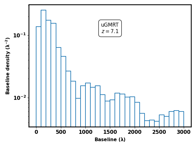


Figure 4 shows simulated visibilities corresponding to the 2D central HI 21-cm map around the ionized bubble centered at . The top left and top right panels show plots of the signal as a function of baseline and frequency respectively, for the uGMRT and the bottom panels display results for the SKA1-Low. We also compare the simulated visibility with the analytical estimation assuming a perfectly spherical ionized bubble of comoving radius Mpc and surrounded by uniform and fully neutral medium (refer to equation 3.7). The IGM around the ionized bubble in simulated maps is not uniform, but traces the underlying DM distribution and is also filled with many small ionized bubbles. This causes HI density to fluctuate and consequently, the visibility signal also fluctuates as a function of baseline and frequency. We see in Figure 4 that the HI fluctuations are stronger at lower baselines which reflects the fact that HI power spectrum (or equivalently the visibility-visibility correlations) increases at lower -modes or baselines [61, 34]. We further see that the fluctuating HI outside the bubble dominates over the visibilities solely due to the HI 21-cm signal around a spherical ionized bubble which is buried in a uniform HI background. Visibilities are similar for the second scenario at for both experiments and we do not show them here explicitly.


3.5 System noise
To make our study more realistic, we introduce system noise contribution from radio interferometers in our simulated mock visibility data. The system noise contribution to the measured visibility in each baseline and frequency channel is an independent Gaussian random variable with zero mean and the root mean square [33]
| (3.9) |
where represents the total system temperature, is the effective collecting area of the antenna, and and denote the channel width and correlator integration time, respectively.
For the uGMRT, K and K/Jy [59] at frequency MHz. The estimated root mean square noise in visibility is approximately for frequency channel width () of kHz and integration time () of seconds in each baseline. K and K/Jy for the SKA1-Low at the same frequency considering antenna efficiency factor unity. and change to K and K/Jy for the SKA1-Low at MHz frequency. For the uGMRT, these numbers are K and K/Jy [59] respectively at MHz frequency. We note that the rms noise will be reduced by a factor of where is the total observation time.
Our mock simulation considers hrs of observations with s and s integration time for the uGMRT and SKA1-Low respectively. This produces a total of and baselines for the uGMRT and SKA1-Low respectively. Lower integration time will produce a higher number of baselines for the SKA1-Low and hence will increase the requirement of computational resources which is beyond our reach. The system noise contribution for hrs of observations will be too high to detect the HI 21-cm signal around the individual ionized bubbles. Therefore, we present our results for and hrs of uGMRT observations at redshifts and , respectively, assuming a total of and nights of observations, with each night lasting hours. Further, for the third scenario, we present the results at redshift for hours, assuming nights of observations. The increased observing time for the third scenario is due to the lower mean neutral hydrogen fraction outside the targeted bubble. Assuming all nights are the same, we reduce the system noise corresponding to an hrs observation by a factor of , , and for the three scenarios, respectively. The resulting mock signal becomes equivalent to , , and hours of uGMRT observations. Similarly, for the SKA1-Low we present our results for hrs of observation for the first two cases at redshift and (neutral hydrogen fraction ) and for hrs of observation for the third case at redshift (neutral hydrogen fraction ). Eventually, we obtain mock visibility data with all the signal contributions (HI 21-cm signal, galactic foreground, extragalactic point sources, and system noise contribution) typical of the uGMRT and SKA1-Low observations.
Figure 5 shows the mock visibility data comprising of HI signal, diffused galactic foreground contribution, and system noise as a function of frequency for two baselines (top left panel) and (top right panel) for the uGMRT at MHz. The corresponding mock visibility for the SKA1-Low is shown in the bottom panels (bottom left panel: , and bottom right panel: ). They also show diffused galactic foreground contributions (red dashed lines). We see that the diffused galactic foreground dominates over the HI 21-cm signal and system noise at a small baseline (left panel) and, at a large baseline (right panel) the system noise dominates over the other two components. The HI 21-cm signal remains buried under the stronger foreground and system noise contributions.


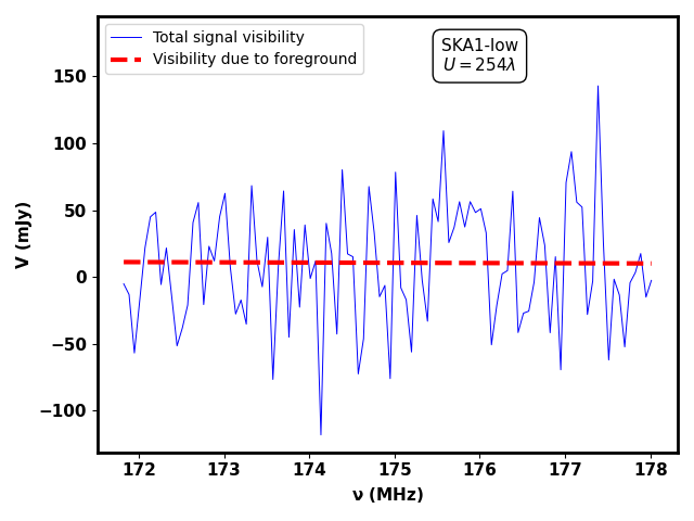
Figure 6 shows the total mock visibility comprising of HI signal, diffused galactic synchrotron emission, radiation from extra-galactic radio point sources, and system noise as a function of frequency for two baselines (left panel) and (right panel) for the uGMRT at MHz. We note that Figure 6 shows contribution both from the extragalactic point sources, galactic diffuse synchrotron radiation along with other components unlike Fig. 5 which shows galactic diffuse synchrotron emission only as the foreground component. The radio point sources are modeled using a simplistic power-law form as discussed in subsection 3.2.1. The green lines indicate visibilities due to point sources. We see that at a small baseline (left panel) the diffuse galactic synchrotron emission dominates over the point sources; at a large baseline (right panel), the point sources dominate over the diffuse galactic synchrotron emission. The total mock visibilities are similar for the second scenario at for both experiments, except for the fact that the system noise and foreground contributions are higher. Therefore, we do not show them here explicitly. The subsequent section discusses the subtraction of the foreground contribution.
Here, we would like to note that the visibility data used in this study does not contain calibration errors, ionospheric effects, and radio-frequency interference (RFI). A comprehensive investigation of these factors will be addressed in future work.


4 Detecting individual ionized bubble in HI 21-cm maps
4.1 Foreground subtraction
The foreground contributions are anticipated to be several orders of magnitude higher than the HI 21-cm signal around ionized bubbles during the EoR. Therefore, one significant challenge is reliably subtracting the foreground signal from the observed signal. All foreground mitigation techniques use the fact that the foregrounds are smooth along the frequency [62, 63]. As discussed earlier, the foreground signal in our simulated mock data has also been assumed to be smooth along frequency. To mitigate foreground components, we fit the total mock visibility signal with a order polynomial of observing frequency as follows,
| (4.1) |
where parameters , , , and are constant. Then, we find the best-fit polynomial along each line of sight corresponding to a baseline and subsequently subtract them from the total simulated mock visibility signal.


Figure 7 presents the residual visibility at 175 MHz after the foreground contribution is subtracted from the total mock visibility for the uGMRT (top panels) and the SKA1-Low (bottom panels). Here, we have only considered the diffuse galactic synchrotron emission as the foreground contamination. However, we get a very similar residual signal when we perform similar analysis on the total mock visibilities considering the radio point source contribution, which has been shown in Figure 9. The residual signal contains the HI 21-cm signal, the system noise, and the un-subtracted foreground, if any. To assess the reliability of foreground subtraction, we compare the combined input HI 21-cm signal and system noise with the extracted signal for two different baselines (top left panel) and (top right panel), as depicted in Figure 8. In the bottom panels of Figure 8, we show a similar comparison for SKA1-Low for two different baselines (bottom left panel) and (bottom right panel). The plots show that the residual visibility closely matches the input visibility data, with only minor deviations. These slight deviations are possibly due to some residual foreground contribution and subtraction of the HI 21-cm signal and the system noise during the foreground subtraction. Consequently, we can conclude that we have mostly subtracted the foreground data from the mock visibility data, making it ready for further analysis, such as matched filtering. We do not present similar results for the second scenario at as it is similar to the first scenario.


4.2 Matched filter
The residual mock visibility (see Figure 7) contains mainly the HI 21-cm signal around the ionized bubble and the system noise from radio interferometers. We see that the dominance of system noise over the HI 21-cm signal is so pronounced that the latter’s presence is barely discernible. Here, we employ a matched filter technique to maximize the signal-to-noise ratio, thereby enhancing the prospects of detecting the HI 21-cm signal around an ionized bubble. The functional form of the visibility signal corresponding to neutral hydrogen around a spherical ionized bubble is quite well known (refer to eq. 3.7). Additionally, the system noise is anticipated to follow a Gaussian random distribution. These conditions enable us to implement the matched filter-based technique effectively. Below, we briefly summarize the method proposed in [33] and consider the following estimator for detecting ionized bubbles from the HI 21-cm signal, which is given as
| (4.2) |
Here, is the filter which is a function of both baseline and frequency . is the total observed visibility which consists of the desired HI 21-cm signal, residual foregrounds, system noise, etc. Here, and refer to the different baselines and frequency channels in our observations. Here, we note that foreground components are subtracted from the total observed visibilities and we employ the matched filtering technique only on the residual visibility which contains only the HI 21-cm signal and system noise. Figure 3 shows a typical uGMRT and SKA1-Low baseline distribution for hrs of observations. We note that the estimator is calculated by taking the sum over all baselines and frequency channels. We get one estimator for a given filter. The contribution of the system noise to the estimator is expected to be zero if it is averaged over a large number of independent realizations. However, for a single realization of the system noise, the contribution of it is unlikely to be exactly zero. It would change for different realizations of the system noise. Therefore, we estimate the variance of the estimator due to the system noise using the following equation [33],
| (4.3) |
Here, is the variance of the system noise for single visibility and can be calculated using eq. 3.9. The symbol denotes summation over all baselines and frequency channels. We note that the variance to the estimator depends on the chosen filter, system noise, and baseline distribution but not on the desired signal. The signal-to-noise ratio (SNR) of a particular detection (or non-detection) can be calculated as,
| (4.4) |
In this work, we consider as the threshold for detection. We would like to mention that the SNR reaches its maximum when the selected filter exactly (or closely) matches with the HI 21-cm signal which is contaminated by the system noise. Therefore, the chosen filter has the same functional form as the HI 21-cm signal around an ionized bubble (refer to eq. 3.7). It also has one free parameter i.e., the radius of the ionized bubble . We assume that the location of the bubble is known a priori from other observations. To find a filter that matches the targeted signal, one needs to explore the entire possible ranges of all parameters (here the size of the targeted bubble). The particular set of parameters yielding the maximum SNR will reveal the size of the ionized bubble in the observed HI 21-cm signal.
5 Results
5.1 Detectability of the QSO ionized bubble at
Here, we present our findings regarding the detectability of ionized bubbles around bright QSO/galaxies in HI 21-cm maps, employing the matched filter technique. We assume that the targeted ionized bubble is located at the antenna phase center. Thus, we simulate the targeted ionized bubble at the center of the simulation cube. Subsequently, we apply the matched filtering technique to the residual visibility obtained after subtracting foreground contaminants. As explained above the residual visibility contains the HI 21-cm signal, system noise, and unsubtracted foregrounds. First, we calculate the estimator using equation 4.2. Because the actual size of the targeted ionized bubble is not known in real observations we calculate the estimator for various filter sizes ranging from to Mpc. Subsequently, we estimate the variance of the estimator due to the system noise using equation 3.9 and the signal to noise ratio (SNR, refer to eq. 4.4) for the same range of filter sizes. Figure 10 shows the resulting SNR as a function of filter size for hrs of uGMRT observation (left panel) and hrs of SKA1-Low observations (right panel) at .

The ten different curves in Figure 10 represent the SNR for ten independent realizations of the system noise. We see that for both the uGMRT and the SKA1-Low, the SNR peaks at filter size Mpc, with minor deviations in different noise realizations. As per the principle of the matched filter technique, the SNR peaks when the filter matches the actual targeted signal (i.e., the HI 21-cm signal around the ionized bubble) in the simulated HI maps. Therefore, we can conclude that the extracted radius of the ionized bubble in the simulated HI 21-cm map is around Mpc. We want to note that the actual radius of the ionized bubble measured directly from the simulated map is Mpc, which is very close to the extracted ones using the matched filter technique. The location of the peak in the SNR curve shifts around the mean value for different realizations, which we shall discuss in detail in the next section.
Further, we see that peak SNR values in all the ten realizations are for hrs of observations with the uGMRT and for hrs of observations with the SKA1-Low. We assume a total bandwidth of MHz and MHz while subtracting the foreground for the uGMRT and SKA1-Low, respectively. The choice of smaller bandwidth for the SKA1-Low is solely due to the limited computational resources available. Use of the higher bandwidth for the SKA1-Low would have subtracted the HI 21-cm signal less during the foreground subtraction process, thus increasing the SNR. Subsection 5.4 discusses the impact of foreground subtraction in more detail. The higher SNR obtained in our results indicates that it is possible to significantly detect individual ionized bubbles in the HI 21-cm maps using the uGMRT with hrs observations and using the SKA1-Low with only around hrs of observations.


To assess the significance of the above result, we estimate the SNR for independent realizations of the system noise for the uGMRT and independent realizations for SKA1-Low, while keeping the HI 21-cm signal and foreground components the same. Figure 10 shows the SNR for some of these realizations for the uGMRT (left panel) and SKA1-Low (right panel) at . The left panel of Figure 11 shows the corresponding mean SNR and spread for all realizations of the uGMRT, while the right panel shows the same for the SKA1-Low with realizations. We see that all the realizations show a peak in the SNR. In principle, the peak should appear at the actual ionized bubble size of Mpc. However, the peak location varies in the range of Mpc and Mpc for the uGMRT and SKA1-Low, respectively, for different realizations. It can be seen in Figure 12, which shows a histogram of peak locations for realizations for the uGMRT.

We see that, although in most cases, the peak is in the range of Mpc for the uGMRT, some extreme realizations show peaks at higher/lower filter radii. The peak value of the SNR for the uGMRT also changes in the range of . Due to much lower system noise and higher sensitivity, the SKA1-Low should be able to detect the ionized bubble with reduced observing time and higher SNR. The estimated bubble size is also highly accurate for the SKA1-Low, which we do not explicitly show here. We note that the above analysis considers only the DGSE as the foreground contaminant. However, we have repeated the analysis including contributions from both the DGSE and radio point sources as foregrounds. We find very similar results to those presented here. Therefore, we do not explicitly show the outcomes of the combined foreground contamination here.
5.2 Detectability of the ionized bubble at
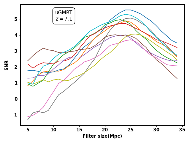
Unlike the ionized bubble at , mainly created by a bright QSO, the bubble at is produced by a collection of galaxies as indicated in [17]. This ionized bubble is relatively more aspherical in shape than at . Figure 13 presents the SNR as a function of filter size for 3072 hrs of uGMRT (left panel) and hrs of SKA1-Low (right panel) observations at .


Different curves are for different independent noise realizations. The system temperature is higher at compared to . Therefore, the SNR decreases at a higher redshift for the same observation time. We see that for both the uGMRT and the SKA1-Low, the SNR peaks at a filter size Mpc, with minor deviations in different noise realizations. It is very close to the actual radius of the ionized bubble measured directly from the simulated map, which is Mpc.
Further, we see that peak SNR values in all ten realizations are for the uGMRT and for the SKA1-Low. Like the previous case, we assume a total bandwidth of MHz and MHz while subtracting the foreground for the uGMRT and SKA1-Low, respectively. We see that it is possible to reliably detect individual ionized bubbles in the HI 21-cm maps using the uGMRT with hrs of observation time and the SKA1-Low with only hrs of observations at .
The left panel of Figure 14 shows the mean SNR along with the spread for noise realizations of the uGMRT, while the right panel shows the same for the SKA1-Low with realizations at . Further, the peak location varies between and Mpc for the uGMRT for different realizations (Figure 13), which can be seen in Figure 15, which shows a histogram of peak locations for realizations for the uGMRT. The peak value of the SNR for the uGMRT also changes in the range of and for the SKA1-Low.


5.3 Detectability of the QSO ionized bubble at for
Here, we present our findings for the third case, where the targeted ionized bubble is surrounded by other ionized regions which result in a lower neutral hydrogen fraction of . Further, the targeted bubble at the center also became aspherical. A lower neutral hydrogen fraction means that the background HI 21-cm signal is weaker, which results in a lower SNR value. We use the same matched filtering technique as described earlier but increased the observation time to hours for the uGMRT and hours for the SKA1-Low, considering the lower SNR and increased difficulty in detecting ionized regions at a lower neutral fraction. Figure 16 shows the SNR as a function of filter size for hours of uGMRT observation (left panel) and hours of SKA1-Low observations (right panel) at . As in previous cases, each curve represents a different noise realization. We see that for the uGMRT, the SNR peaks at a filter size Mpc, and for the SKA1-Low, it peaks at Mpc, with minor deviations in different noise realizations.


Further, we see that peak SNR values in all ten realizations are for the uGMRT and for the SKA1-Low. Like the previous cases, we assume a total bandwidth of MHz and MHz while subtracting the foreground for the uGMRT and SKA1-Low, respectively. We see that it is possible to reliably detect individual ionized bubbles in the HI 21-cm maps using the uGMRT with hours of observation time and the SKA1-Low with only hours of observations at with significantly much lower neutral hydrogen fraction value.


The left panel of Figure 17 shows the mean SNR along with the spread for noise realizations of the uGMRT, while the right panel shows the same for the SKA1-Low with realizations at for . Further, the peak location varies between and Mpc for the uGMRT for different realizations (Figure 16), which can be seen in Figure 18, that shows a histogram of peak locations for realizations for the uGMRT. The peak value of the SNR for the uGMRT also changes in the range of and for the SKA1-Low.
5.4 Impact of foreground subtraction

We noticed that during the process of foreground subtraction using a polynomial along the frequency axis, a small part of the HI 21-cm signal also gets subtracted along with the foreground. It reduces the SNR to some extent. We further notice that the amount of subtraction of the HI 21-cm signal depends on the frequency bandwidth used during the foreground subtraction process. The fraction of HI 21-cm signal subtracted is more for smaller bandwidth compared to the case when larger frequency bandwidth is used. Consequently, the drop in the SNR is more significant for smaller bandwidths. Figure 19 shows the SNR as a function of the bandwidth for hrs of observations with uGMRT at . We see that the SNR, which is lower than at MHz bandwidth, increases to when MHz bandwidth is assumed. Here, we note that the SNR reaches for the above observation when no foreground is used and the process of foreground subtraction is skipped. Therefore, the SNR is reduced by percent when the bubble size is Mpc, and MHz bandwidth is assumed for foreground subtraction. Using higher bandwidth during the foreground subtraction would enhance the SNR and prospects of ionized bubble detection. However, increased bandwidth will increase the computational cost during the analysis. We find similar results for the SKA1-Low but do not explicitly show them here. The impact of foreground subtraction on the SNR will also depend on the foreground subtraction methods, and therefore, a thorough investigation is required.
5.5 Constraining the neutral hydrogen fraction
We see that the visibility corresponding to the HI 21-cm signal around a spherical ionized bubble in the IGM is proportional to the mass-averaged neutral hydrogen fraction of the IGM outside the bubble (refer to eq. 3.7). One can further show that [36],
| (5.1) |
where depends on the bubble size, redshift, and various observational parameters such as the , total number of antennae, observing time, antenna collecting area, and baseline distribution. All these quantities are constant at a fixed redshift. One can use this relation to place constraints on . Now, we focus on the ionized bubble around the QSO at and hrs of observation time with uGMRT. The SNR value changes for different noise realizations in Figure 10 (left panel). The average SNR value peaks at (Figure 11) at the filter size 23 Mpc for the uGMRT at . Further, we see that uncertainty in the SNR value at the same filter size is 0.73. Therefore, we estimate the hydrogen neutral fraction using , where the SNR and is measured at the peak location.
To calculate , we simulate an entirely neutral and uniform HI 21-cm signal around a spherical ionized bubble of radius 23 Mpc, i.e., outside the ionized bubble. It allows us to estimate using eq. 5.1. Now, after adding the foreground component only with the HI 21-cm signal, we follow the entire analysis and calculate the SNR as a function of filter size without adding system noise from the radio interferometers. The SNR, in this case, peaks at 23 Mpc and is supposed to be equal to (following eq. 5.1) as the outside the ionized bubble in this case. We use this value of to estimate the mean and the uncertainty associated with it. The estimated neutral fraction is at for hrs of observations with uGMRT. It is very close to the actual in the simulation, which is . The estimated upper limit of exceeds unity which is, of course, unrealistic. The SKA1-Low places much tighter constraints, which is using only hrs of observations for the same scenario. Similarly we also studied this for the third case, where the neutral hydrogen fraction is lower in the simulation, discussed in subsection 5.3. We find the estimated neutral hydrogen fraction to be at for hours of observations with the uGMRT, which is very close to the actual neutral hydrogen fraction .
The above result demonstrates the prospects of constraining the mass-averaged neutral fraction using the technique discussed in this work. The SKA1-Low is expected to put much tighter constraints on the . A thorough analysis is required considering different bubble sizes and hydrogen neutral fractions at different redshifts for various instruments, and we leave this exercise for future work.
6 Summary & Discussion
Several bright QSOs/galaxies have recently been detected at . We expect large ionized bubbles, with comoving sizes of tens of Mpc, around these sources, which are embedded in a neutral HI medium. We have conducted a detailed investigation into the prospects of detecting such individual ionized bubbles using observations of the HI 21-cm signal from the epoch of reionization by the uGMRT and SKA1-Low. We have mainly focused on two known sources: one very bright QSO at [8] and a large ionized bubble around a collection of galaxies at redshift [17].
First, we simulated the HI 21-cm signal around bright QSOs/galaxies matching the above cases and foreground contaminants in a 3D cube. Subsequently, we have generated visibilities corresponding to the HI 21-cm signal and foregrounds at baselines similar to the uGMRT and SKA1-Low experiments and added the system noise with the visibilities corresponding to the HI signal and foreground contaminants. We then employ a foreground mitigation technique based on a polynomial fitting algorithm to remove them from the total visibilities. The residual visibilities match well with the combination of the input HI signal and system noise. However, it is heavily dominated by the system noise. To minimize the effects of system noise in the estimated quantity, we employed a technique based on the matched filter algorithm. This technique is applicable in our case as the functional form of the desired HI 21-cm signal around bright sources is known. We find that the expected signal-to-noise ratio for the proposed estimator for the uGMRT is for both hours of observations at redshift and hours at redshift , when the mean HI fraction outside the targeted bubble is . However, the required observing time increases to hrs for the uGMRT at redshift to achieve a similar SNR when the mean HI fraction is lower at . The SKA1-Low will have a much higher SNR () with just hrs of observations at same redshifts and , when the mean HI fraction outside the targeted bubble is . However, the required observing time increases to hrs for the SKA1-Low at redshift to achieve a similar SNR when the mean HI fraction is lower at .
Apart from detecting the HI 21-cm signal, the technique is also able to measure the size of the ionized regions and HI neutral fraction. For the uGMRT hours of observations at redshift , we find that the estimated bubble size ranges between Mpc for independent noise realizations when the actual bubble size is Mpc. Similar results are obtained for hours of observations with the uGMRT at redshift with a mean HI fraction of and for hours at redshift with a mean HI fraction of . The SKA1-Low should measure the bubble size more accurately, with the uncertainty in bubble size estimation being less than Mpc at both mentioned redshifts.
We have also explored the potential to constrain the neutral hydrogen fraction of the IGM outside the ionized bubble. We find that our technique can either directly measure the neutral hydrogen fraction or put an upper or lower limit on it, depending on the actual neutral fraction and the observational specifications.
The process of foreground subtraction using a polynomial along the frequency axis also removes some of the desired HI signal. We found that the fraction of subtracted HI signal increases when using smaller frequency bandwidth, significantly reducing the signal-to-noise ratio. We thoroughly investigated this effect using a wide range of bandwidths and found that the SNR increases by more than four times when the frequency bandwidth is increased from MHz to MHz for bubble size Mpc. We studied three particular cases here and results may vary if sizes of ionized bubbles and redshifts change. However, our methods can be applied to any similar cases.
Here, we focused on the targeted detection of ionized bubbles around sources previously detected by other telescopes. Several such sources have been observed during the reionization epoch. Additionally, the matched filter technique can detect ionized bubbles even without prior source detection. However, this unguided detection requires exploring a vast parameter space, which is computationally expensive. The underlying bubble may not be spherical, as assumed in our study. However, as long as the bubble is relatively isolated, the method remains applicable, though the SNR might be reduced. Furthermore, we note that our simulations do not account for the contributions of low-mass halos to reionization. This omission likely results in an underestimation of the diffuse and complex structure of the ionized regions. Accurately incorporating these contributions could, to some extent, degrade the predicted signal-to-noise ratio. Foregrounds are assumed to be spectrally smooth here, which may not be accurate in actual observations. A more sophisticated method for foreground mitigation may be needed in case foregrounds behave differently. We would also like to note that this study does not account for potential errors arising from improper calibration [64], ionospheric effects, or radio-frequency interference (RFI). These practical issues will be addressed in future works.
Acknowledgments
AM and CSM acknowledge financial support from Council of Scientific and Industrial Research (CSIR) via CSIR-SRF fellowships under grant no. 09/0096(13611)/2022-EMR-I and 09/1022(0080)/2019-EMR-I respectively. KKD acknowledges financial support from SERB (Govt. of India) through a project under MATRICS scheme (MTR/2021/000384). SM acknowledges financial support through the project titled “Observing the Cosmic Dawn in Multicolour using Next Generation Telescopes” funded by the Science and Engineering Research Board (SERB), Department of Science and Technology, Govt. of India through the Core Research Grant No. CRG/2021/004025. The authors acknowledge the use of computational resources available to the Inter-University Centre for Astronomy and Astrophysics (IUCAA), Pune, and to the Cosmology with Statistical Inference (CSI) research group at the Indian Institute of Technology Indore (IIT Indore).
References
- [1] R. Barkana and A. Loeb, In the beginning: the first sources of light and the reionization of the universe, Physics Reports 349 (2001) 125.
- [2] A. Loeb, Frontmatter, in How Did the First Stars and Galaxies Form?, (Princeton), pp. i–vi, Princeton University Press (2010), DOI.
- [3] J.R. Pritchard and A. Loeb, 21 cm cosmology in the 21st century, Reports on Progress in Physics 75 (2012) 086901.
- [4] A. Bera, R. Ghara, A. Chatterjee, K.K. Datta and S. Samui, Studying cosmic dawn using redshifted HI 21-cm signal: A brief review, Journal of Astrophysics and Astronomy 44 (2023) 10 [2210.12164].
- [5] G. Mellema, I.T. Iliev, U.-L. Pen and P.R. Shapiro, Simulating cosmic reionization at large scales - II. The 21-cm emission features and statistical signals, Monthly Notices of the Royal Astronomical Society 372 (2006) 679 [astro-ph/0603518].
- [6] S.R. Furlanetto, S.P. Oh and F.H. Briggs, Cosmology at low frequencies: The 21cm transition and the high-redshift universe, Physics Reports 433 (2006) 181.
- [7] T.R. Choudhury, M.G. Haehnelt and J. Regan, Inside-out or outside-in: the topology of reionization in the photon-starved regime suggested by Ly forest data, Monthly Notices of the Royal Astronomical Society 394 (2009) 960 [0806.1524].
- [8] D.J. Mortlock, S.J. Warren, B.P. Venemans, M. Patel, P.C. Hewett, R.G. McMahon et al., A luminous quasar at a redshift of z = 7.085, Nature 474 (2011) 616–619.
- [9] X.-B. Wu, X.-B. Wu, F. Wang, F. Wang, F. Wang, X. Fan et al., An ultraluminous quasar with a twelve-billion-solar-mass black hole at redshift 6.30, Nature (2015) .
- [10] E. Bañados, B.P. Venemans, C. Mazzucchelli, E.P. Farina, F. Walter, F. Wang et al., An 800-million-solar-mass black hole in a significantly neutral universe at a redshift of 7.5, Nature 553 (2017) 473–476.
- [11] F. Wang, J. Yang, X. Fan, M. Yue, X.-B. Wu, J.-T. Schindler et al., The discovery of a luminous broad absorption line quasar at a redshift of 7.02, The Astrophysical Journal Letters 869 (2018) L9.
- [12] F. Wang, J. Yang, X. Fan, X.-B. Wu, M. Yue, J.-T. Li et al., Exploring Reionization-era Quasars. III. Discovery of 16 Quasars at 6.4 z 6.9 with DESI Legacy Imaging Surveys and the UKIRT Hemisphere Survey and Quasar Luminosity Function at z 6.7, The Astrophysical Journal 884 (2019) 30 [1810.11926].
- [13] Y. Matsuoka, M. Onoue, N. Kashikawa, M.A. Strauss, K. Iwasawa, C.-H. Lee et al., Discovery of the First Low-luminosity Quasar at z ¿ 7, The Astrophysical Journal Letters 872 (2019) L2 [1901.10487].
- [14] J. Yang, F. Wang, X. Fan, J.F. Hennawi, F.B. Davies, M. Yue et al., Pōniuā‘ena: A luminous z = 7.5 quasar hosting a 1.5 billion solar mass black hole, The Astrophysical Journal Letters 897 (2020) L14.
- [15] F. Wang, J. Yang, X. Fan, J.F. Hennawi, A.J. Barth, E. Banados et al., A luminous quasar at redshift 7.642, The Astrophysical Journal Letters 907 (2021) L1.
- [16] Y. Matsuoka, K. Iwasawa, M. Onoue, N. Kashikawa, M.A. Strauss, C.-H. Lee et al., Subaru High-z Exploration of Low-luminosity Quasars (SHELLQs). X. Discovery of 35 Quasars and Luminous Galaxies at 5.7 z 7.0, The Astrophysical Journal 883 (2019) 183 [1908.07910].
- [17] J. Witstok, R. Maiolino, R. Smit, G.C. Jones, A.J. Bunker, J.M. Helton et al., JADES: Primeval Lyman- emitting galaxies reveal early sites of reionisation out to redshift , arXiv e-prints (2024) arXiv:2404.05724 [2404.05724].
- [18] G. Mellema, L.V.E. Koopmans, F.A. Abdalla, G. Bernardi, B. Ciardi, S. Daiboo et al., Reionization and the Cosmic Dawn with the Square Kilometre Array, Experimental Astronomy 36 (2013) 235 [1210.0197].
- [19] S. Majumdar, S. Bharadwaj, K.K. Datta and T.R. Choudhury, The impact of anisotropy from finite light traveltime on detecting ionized bubbles in redshifted 21-cm maps, Monthly Notices of the Royal Astronomical Society 413 (2011) 1409 [1006.0430].
- [20] S. Majumdar, S. Bharadwaj and T.R. Choudhury, Constrainingquasar and intergalactic medium properties through bubble detection in redshifted 21-cm maps, Monthly Notices of the Royal Astronomical Society 426 (2012) 3178 [1111.6354].
- [21] R. Ghara, T.R. Choudhury, K.K. Datta and S. Choudhuri, Imaging the redshifted 21 cm pattern around the first sources during the cosmic dawn using the SKA, Monthly Notices of the Royal Astronomical Society 464 (2017) 2234 [1607.02779].
- [22] E. Zackrisson, S. Majumdar, R. Mondal, C. Binggeli, M. Sahlén, T.R. Choudhury et al., Bubble mapping with the Square Kilometre Array - I. Detecting galaxies with Euclid, JWST, WFIRST, and ELT within ionized bubbles in the intergalactic medium at z ¿ 6, Monthly Notices of the Royal Astronomical Society 493 (2020) 855 [1905.00437].
- [23] S.K. Giri, G. Mellema and R. Ghara, Optimal identification of H II regions during reionization in 21-cm observations, Monthly Notices of the Royal Astronomical Society 479 (2018) 5596 [1801.06550].
- [24] S.K. Giri, G. Mellema, K.L. Dixon and I.T. Iliev, Bubble size statistics during reionization from 21-cm tomography, Monthly Notices of the Royal Astronomical Society 473 (2018) 2949 [1706.00665].
- [25] M. Bianco, S.K. Giri, D. Prelogović, T. Chen, F.G. Mertens, E. Tolley et al., Deep learning approach for identification of H II regions during reionization in 21-cm observations - II. Foreground contamination, Monthly Notices of the Royal Astronomical Society 528 (2024) 5212 [2304.02661].
- [26] M. Bianco, S.K. Giri, R. Sharma, T. Chen, S. Parth Krishna, C. Finlay et al., Deep learning approach for identification of HII regions during reionization in 21-cm observations – III. image recovery, arXiv e-prints (2024) arXiv:2408.16814 [2408.16814].
- [27] T. Di Matteo, R. Perna, T. Abel and M.J. Rees, Radio Foregrounds for the 21 Centimeter Tomography of the Neutral Intergalactic Medium at High Redshifts, The Astrophysical Journal 564 (2002) 576 [astro-ph/0109241].
- [28] S.P. Oh and K.J. Mack, Foregrounds for 21-cm observations of neutral gas at high redshift, Monthly Notices of the Royal Astronomical Society 346 (2003) 871 [astro-ph/0302099].
- [29] M.G. Santos, A. Cooray and L. Knox, Multifrequency Analysis of 21 Centimeter Fluctuations from the Era of Reionization, The Astrophysical Journal 625 (2005) 575 [astro-ph/0408515].
- [30] S.S. Ali, S. Bharadwaj and J.N. Chengalur, Foregrounds for redshifted 21-cm studies of reionization: Giant meter wave radio telescope 153-mhz observations, Monthly Notices of the Royal Astronomical Society 385 (2008) 2166–2174.
- [31] P.M. Geil, J.S.B. Wyithe, N. Petrovic and S.P. Oh, The effect of Galactic foreground subtraction on redshifted 21-cm observations of quasar HII regions, Monthly Notices of the Royal Astronomical Society 390 (2008) 1496 [0805.0038].
- [32] K. Kakiichi, S. Majumdar, G. Mellema, B. Ciardi, K.L. Dixon, I.T. Iliev et al., Recovering the H II region size statistics from 21-cm tomography, Monthly Notices of the Royal Astronomical Society 471 (2017) 1936 [1702.02520].
- [33] K.K. Datta, S. Bharadwaj and T.R. Choudhury, Detecting ionized bubbles in redshifted 21-cm maps, Monthly Notices of the Royal Astronomical Society 382 (2007) 809.
- [34] K.K. Datta, S. Majumdar, S. Bharadwaj and T.R. Choudhury, Simulating the impact of h i fluctuations on matched filter search for ionized bubbles in redshifted 21-cm maps, Monthly Notices of the Royal Astronomical Society 391 (2008) 1900.
- [35] K.K. Datta, M.M. Friedrich, G. Mellema, I.T. Iliev and P.R. Shapiro, Prospects of observing a quasar H II region during the epoch of reionization with the redshifted 21-cm signal, Monthly Notices of the Royal Astronomical Society 424 (2012) 762 [1203.0517].
- [36] K.K. Datta, S. Bharadwaj and T.R. Choudhury, The optimal redshift for detecting ionized bubbles in h¡scp¿i¡/scp¿ 21-cm maps, Monthly Notices of the Royal Astronomical Society: Letters 399 (2009) L132–L136.
- [37] R. Ghara and T.R. Choudhury, Bayesian approach to constraining the properties of ionized bubbles during reionization, Monthly Notices of the Royal Astronomical Society 496 (2020) 739 [1909.12317].
- [38] A. Mesinger, B. Greig and E. Sobacchi, The Evolution Of 21 cm Structure (EOS): public, large-scale simulations of Cosmic Dawn and reionization, Monthly Notices of the Royal Astronomical Society 459 (2016) 2342 [1602.07711].
- [39] S. Majumdar, J.R. Pritchard, R. Mondal, C.A. Watkinson, S. Bharadwaj and G. Mellema, Quantifying the non-Gaussianity in the EoR 21-cm signal through bispectrum, Monthly Notices of the Royal Astronomical Society 476 (2018) 4007 [1708.08458].
- [40] S. Majumdar, M. Kamran, J.R. Pritchard, R. Mondal, A. Mazumdar, S. Bharadwaj et al., Redshifted 21-cm bispectrum - I. Impact of the redshift space distortions on the signal from the Epoch of Reionization, Monthly Notices of the Royal Astronomical Society 499 (2020) 5090 [2007.06584].
- [41] C.M. Trott, C.A. Watkinson, C.H. Jordan, S. Yoshiura, S. Majumdar, N. Barry et al., Gridded and direct Epoch of Reionisation bispectrum estimates using the Murchison Widefield Array, Publications of the Astronomical Society of Australia 36 (2019) e023 [1905.07161].
- [42] R. Ghara, S.K. Giri, G. Mellema, B. Ciardi, S. Zaroubi, I.T. Iliev et al., Constraining the intergalactic medium at z 9.1 using LOFAR Epoch of Reionization observations, Monthly Notices of the Royal Astronomical Society 493 (2020) 4728 [2002.07195].
- [43] M. Kamran, R. Ghara, S. Majumdar, R. Mondal, G. Mellema, S. Bharadwaj et al., Redshifted 21-cm bispectrum - II. Impact of the spin temperature fluctuations and redshift space distortions on the signal from the Cosmic Dawn, Monthly Notices of the Royal Astronomical Society 502 (2021) 3800 [2012.11616].
- [44] L. Noble, M. Kamran, S. Majumdar, C. Shekhar Murmu, R. Ghara, G. Mellema et al., Impact of the Epoch of Reionization sources on the 21-cm bispectrum, arXiv e-prints (2024) arXiv:2406.03118 [2406.03118].
- [45] C.L. Bennett, D. Larson, J.L. Weiland, N. Jarosik, G. Hinshaw, N. Odegard et al., Nine-year wilkinson microwave anisotropy probe ( wmap ) observations: Final maps and results, The Astrophysical Journal Supplement Series 208 (2013) 20.
- [46] S. Bharadwaj and S.S. Ali, The cosmic microwave background radiation fluctuations from h i perturbations prior to reionization, Monthly Notices of the Royal Astronomical Society 352 (2004) 142.
- [47] S. Bharadwaj and S.S. Ali, On using visibility correlations to probe the h i distribution from the dark ages to the present epoch - i. formalism and the expected signal, Monthly Notices of the Royal Astronomical Society 356 (2005) 1519.
- [48] S.A. Wouthuysen, On the excitation mechanism of the 21-cm (radio-frequency) interstellar hydrogen emission line., The Astronomical Journal 57 (1952) 31.
- [49] G.B. Field, Excitation of the Hydrogen 21-CM Line, Proceedings of the IRE 46 (1958) 240.
- [50] P. Madau, A. Meiksin and M.J. Rees, 21 Centimeter Tomography of the Intergalactic Medium at High Redshift, The Astrophysical Journal 475 (1997) 429 [astro-ph/9608010].
- [51] S. Bharadwaj and P.S. Srikant, HI fluctuations at large redshifts: III — simulating the signal expected at GMRT, Journal of Astrophysics and Astronomy 25 (2004) 67.
- [52] R. Mondal, S. Bharadwaj, S. Majumdar, A. Bera and A. Acharyya, The effect of non-Gaussianity on error predictions for the Epoch of Reionization (EoR) 21-cm power spectrum, Monthly Notices of the Royal Astronomical Society: Letters 449 (2015) L41 [https://academic.oup.com/mnrasl/article-pdf/449/1/L41/9419984/slv015.pdf].
- [53] T.R. Choudhury, M.G. Haehnelt and J. Regan, Inside-out or outside-in: the topology of reionization in the photon-starved regime suggested by Ly-alpha forest data, Monthly Notices of the Royal Astronomical Society 394 (2009) 960 [https://academic.oup.com/mnras/article-pdf/394/2/960/3710519/mnras0394-0960.pdf].
- [54] S. Majumdar, G. Mellema, K.K. Datta, H. Jensen, T.R. Choudhury, S. Bharadwaj et al., On the use of seminumerical simulations in predicting the 21-cm signal from the epoch of reionization, Monthly Notices of the Royal Astronomical Society 443 (2014) 2843 [https://academic.oup.com/mnras/article-pdf/443/4/2843/6274877/stu1342.pdf].
- [55] R. Mondal, S. Bharadwaj and S. Majumdar, Statistics of the epoch of reionization (EoR) 21-cm signal - II. The evolution of the power-spectrum error-covariance, Monthly Notices of the Royal Astronomical Society 464 (2017) 2992 [1606.03874].
- [56] V. Jelić , S. Zaroubi, P. Labropoulos, R.M. Thomas, G. Bernardi, M.A. Brentjens et al., Foreground simulations for the LOFAR-epoch of reionization experiment, Monthly Notices of the Royal Astronomical Society 389 (2008) 1319.
- [57] S. Choudhuri, S. Bharadwaj, A. Ghosh and S.S. Ali, Visibility-based angular power spectrum estimation in low-frequency radio interferometric observations, Monthly Notices of the Royal Astronomical Society 445 (2014) 4351.
- [58] A. Ghosh, J. Prasad, S. Bharadwaj, S.S. Ali and J.N. Chengalur, Characterizing foreground for redshifted 21 cm radiation: 150 MHz Giant Metrewave Radio Telescope observations, Monthly Notices of the Royal Astronomical Society 426 (2012) 3295 [https://academic.oup.com/mnras/article-pdf/426/4/3295/3332953/426-4-3295.pdf].
- [59] Y. Gupta, B. Ajithkumar, H.S. Kale, S. Nayak, S. Sabhapathy, S. Sureshkumar et al., The upgraded GMRT: opening new windows on the radio Universe, Current Science 113 (2017) 707.
- [60] SKA Observatory, “Ska telescope specifications.” https://www.skao.int/en/science-users/118/ska-telescope-specifications#:~:text=SKA1%2DLow%20(also%20referred%20to,stations%20of%20256%20antennas%20each., 2024.
- [61] S. Bharadwaj and S.S. Ali, On using visibility correlations to probe the HI distribution from the dark ages to the present epoch - I. Formalism and the expected signal, Monthly Notices of the Royal Astronomical Society 356 (2005) 1519 [astro-ph/0406676].
- [62] J. Cho and A. Lazarian, Galactic foregrounds: Spatial fluctuations and a procedure for removal, The Astrophysical Journal 720 (2010) 1181.
- [63] F. Martire, R. Barreiro and E. Martínez-González, Characterization of the polarized synchrotron emission from planck and wmap data, Journal of Cosmology and Astroparticle Physics 2022 (2022) 003.
- [64] S. Gayen, R. Sagar, S. Mangla, P. Dutta, N. Roy, A. Chakraborty et al., Calibration requirement for Epoch of Reionization 21-cm signal observation. Part III. Bias and variance in uGMRT ELAIS-N1 field power spectrum, Journal of Cosmology and Astroparticle Physics 2024 (2024) 068 [2402.18306].