Detecting Gravitational-waves from Extreme Mass Ratio Inspirals using Convolutional Neural Networks
Abstract
Extreme mass ratio inspirals (EMRIs) are among the most interesting gravitational wave (GW) sources for space-borne GW detectors. However, successful GW data analysis remains challenging due to many issues, ranging from the difficulty of modeling accurate waveforms, to the impractically large template bank required by the traditional matched filtering search method. In this work, we introduce a proof-of-principle approach for EMRI detection based on convolutional neural networks (CNNs). We demonstrate the performance with simulated EMRI signals buried in Gaussian noise. We show that over a wide range of physical parameters, the network is effective for EMRI systems with a signal-to-noise ratio larger than 50, and the performance is most strongly related to the signal-to-noise ratio. The method also shows good generalization ability towards different waveform models. Our study reveals the potential applicability of machine learning technology like CNNs towards more realistic EMRI data analysis.
I Introduction
The successful detection of Gravitational Waves has opened a new window of understanding the Universe Abbott et al. (2019, 2020, 2021a, 2021b). However, a wide band of GW frequencies is still inaccessible for observation. For example, systems like Double White Dwarfs Huang et al. (2020); Korol et al. (2017), Massive Binary Black Holes Wang et al. (2019); Klein et al. (2016), stellar-mass Binary Black Holes Liu et al. (2020); Sesana (2016), Extreme Mass Ratio Inspirals Babak et al. (2017a); Fan et al. (2020), and stochastic gravitational-wave background Liang et al. (2021); Chen et al. (2019) are expected to emit GW signals in the Hz frequency band. The future detections of these signals can help us better understand the nature of gravity (e.g. Shi et al., 2019; Zi et al., 2021) and the Universe (e.g. Zhu et al., 2021a, b). In order to properly understand the physics and astronomy behind GW events, sophisticated and efficient algorithm to perform data analysis plays a significant role.
Space-borne GW missions are capable of detecting GW signals in the mHz band Luo et al. (2016); Mei et al. (2020). Of all expected GW sources, EMRIs are among the most interesting ones. A typical EMRI system is composed of a stellar-mass Compact Object (CO) and a Massive Black Hole (MBH) (). Such systems are believed to be formed in the center of galaxies. The detection of EMRIs , among other things, can help us better understand the growth mechanism of MBHs, and also put a more stringent constraint on their population properties, like the mass function and the distribution of the surrounding COs Baker et al. (2019); Amaro-Seoane et al. (2007). In addition, the EMRI signal can last for thousands to millions of cycles in the Hz frequency band. This feature empowers the EMRI systems to be ideal laboratories to study gravity in a strong regime. Zi et al. (2021); Moore et al. (2017); Yunes et al. (2012); Canizares et al. (2012); Barack and Cutler (2007).
Despite its great scientific potential, there remain great challenges for the end-to-end data analysis of EMRI signals. For example, the ideal EMRI waveform should consider the effects of self-force. Some progress on self-force waveform has been made recently, such as Lynch et al. (2021) for an eccentric orbit to the second-order, and Isoyama et al. (2021) for a generic orbit to the adiabatic order. However, a fast and accurate EMRI waveform for the most general case is yet to be implemented. Most of the widely used waveform models are expected to quickly dephase from the physical waveform, which restricts its applicability in EMRI data analysis. The computational cost of EMRI waveforms is also usually very high, since it involves orbit integration over a period of months to years. It has been estimated that in order to implement a classical signal search with matched filtering, a bank template containing at least templates would be needed Gair et al. (2004).
Some attempts have been made to explore efficient data analysis algorithms for EMRIs. Both template-based algorithms and template-free methods have been proposed to detect the EMRI signals. The former includes the semi-coherent method Gair et al. (2004) and statistic algorithm Wang et al. (2012, 2015), and the latter includes the time-frequency algorithm Gair and Wen (2005); Wen and Gair (2005); Gair and Jones (2007); Gair et al. (2008a). On the parameter estimation side, methods like Metropolis-Hastings search Gair et al. (2008b); Babak et al. (2009), parallel tempering MCMC Ali et al. (2012), and Gaussian process Chua (2016); Chua et al. (2020) have been implemented.
In recent years, machine learning has gained huge popularity in various complex tasks, such as computer vision Krizhevsky et al. (2012); Simonyan and Zisserman (2014); Szegedy et al. (2015); He et al. (2015); Chollet (2016); Szegedy et al. (2016), speech recognition Deng et al. (2013), natural language process Collobert et al. (2011), and some have been successfully applied to GW astronomy George and Huerta (2018a, b); Huerta et al. (2019); Xia et al. (2020); Gabbard et al. (2018); Schäfer et al. (2020); Krastev et al. (2021); Chan et al. (2020); Bayley et al. (2019, 2020); Gabbard et al. (2019); Williams et al. (2021); George et al. (2017); Shen et al. (2019). Deep learning is a sub-field of machine learning that is based on learning several levels of data representations Heaton (2017), corresponding to a hierarchy of features, factors, or concepts, where higher-level concepts are defined from lower-level ones. The Convolutional Neural Network (CNN) is a deep learning algorithm, which has been applied in many fields because it can automatically extract data features and easily process various high-dimensional data, such as image classification, target detection, and part-of-speech tagging. In GW data analysis, CNNs has been used to detect GW signals detection, such as Binary Black Hole (BBH) mergers George and Huerta (2018a, b); Huerta et al. (2019); Xia et al. (2020); Gabbard et al. (2018), Binary Neutron Star (BNS) mergers Schäfer et al. (2020); Krastev et al. (2021), supernova explosions Chan et al. (2020), and continuous gravitational waves Bayley et al. (2019, 2020). After being properly trained, deep learning methods also demand low computation cost, which improves efficiency in an end-to-end detection system. In this work, we use TianQin, a space-borne GW detector, as a reference, to explore the EMRI signal detection with a CNN.
This paper is organized as follows. Section II introduces the characteristics of EMRI and its waveform. Section III provides the architecture of a CNN, and discusses how to prepare datasets. Section IV describes the search procedure. The results are presented in Section V. Conclusions and discussions are provided in Section VI.
II Basics of EMRI detection
II.1 Basic astronomy of EMRIs
Galactic nuclei are extreme environments for stellar dynamics Amaro-Seoane (2018). The stellar densities can be as high as and its velocity scatter can exceed . Within a galactic nucleus, a large number of COs, including stellar-mass Black Holes, White Dwarfs, and Neutron Stars, are expected to exist. They are considered to be within the “loss cone” if their orbit would lead to their capture by the central MBH, leading to the formation of EMRIs. COs outside the loss cone can fill the loss cone through dynamical processes like two-body relaxation Amaro-Seoane (2018).
In addition to this traditional channel, some new formation channels of EMRI systems have also been proposed. It has been conjectured that a CO can be captured by the accretion disk around central MBH( i.e., Active Galactic Nuclei (AGN) disk). Effects like wind effects, density wave generation, and dynamic friction can assist the inward migration of COs, which further boosts the formation of EMRIs Pan and Yang (2021); Pan et al. (2021).
Although EMRIs are speculated to exist, no direct observational evidence is available yet (c.f.Arcodia et al. (2021)). Therefore, currently, the population properties of EMRIs are derived from theoretical modeling. However, components within the theoretical modeling, like the mass and spin distribution of the central MBH, the erosion of the stellar cusp, the M- relation, etc. are uncertain, which lead to a very uncertain prediction on EMRI population Babak et al. (2017b). Indeed, different assumptions on EMRI population lead to orders of magnitude difference in terms of detection rate by TianQin Fan et al. (2020). Throughout this analysis, an model is adopted to simulate EMRI population. To be exact, we adopt the model M12 from Babak et al. (2017b).
II.2 Waveform models of EMRIs
Theoretical modelling of EMRI waveforms is essential for the successful detection of GWs from these systems. To accurately compute the EMRI waveform, one has to consider the effects of the gravitational self-force, which leads to a deviation of CO orbit from the test particle geodesics under the Kerr metric of the MBH Barack (2009). Unfortunately, waveform simulations with numerical relativity cannot be used for EMRI due to prohibitively high computational costs caused by the very high mass ratio of such systems. Although some progress has been made in adding self-force into the waveform generation Barack (2009); Van De Meent (2018); Miller and Pound (2021); Hughes et al. (2021); McCart et al. (2021); Lynch et al. (2021); Isoyama et al. (2021), a fully realistic solution for EMRI is still yet to be achieved. Nevertheless, there are methods that can generate EMRI waveforms. For example, the Teukolsky-based waveform Hughes et al. (2005) and Numerical Kludge (NK) waveform Babak et al. (2007) solves the Teukolsky equation with the geodesic under Kerr metric. Such methods suffer from low efficiency, while the Analytic Kludge (AK) method that adopts the post-Newtonian (PN) formula can achieve waveform generation in a much faster way Barack and Cutler (2004). The Augmented Analytic Kludge (AAK) waveform Chua and Gair (2015a) can reach an accuracy similar to NK with the generating speed of AK. For our study, since a large number of simulated waveforms are needed for the training, testing, and validation of our CNN method, we focus on the analytic family of waveform models and concentrate on both AK and AAK waveforms. We remark that during the writing of this manuscript, a new and fast waveform has been implemented Katz et al. (2021), which could be used to improve efficiency in the future, but we do not expect any significant difference in our findings. Besides, Katz et al. (2021) adopts the Schwarzschild Black Hole (BH) assumption, while we would like to also study the impact of MBH spin.
The AK method first calculates the orbit of CO through post-Newtonian equations, considering the radiation back-reaction and the Lense-Thirring effect. The overall evolution of the CO orbit is governed by three fundamental frequencies, namely the orbital angular frequency , the periapsis precession frequency , and the Lense-Thirring precession frequency . The waveform is then calculated based on quadrupolar approximation. Notice that the overall setup of a waveform is not self-consistent, hence the name of a “kludge”. However, this choice of formulation allows a fast way of producing waveforms at the cost of its accuracy.
Under the transverse and traceless gauge, two polarizations of AK waveform are defined via a -harmonic waveform which is a function of physical parameters 111The details of the parameters adopted are presented in Table 2:
where is the orbital angular momentum, is the position of the source, and is an azimuthal angle measuring the direction of pericenter. The coefficients () with ranges from 1 to 5, are determined by the eccentricity and mean anomaly orbital phase Barack and Cutler (2004). The orbital phase is determined by three fundamental frequencies and . More details on waveform generation can be found in Barack and Cutler (2004); Fan et al. (2020). Notice that since the self-force can not be properly incorporated by the AK waveform, the spin parameter for the CO is not included.
The AK waveform quickly deviates from physical systems, due to intrinsic inconsistency. Under the AK model, instead of using the physical parameters, one can adopt the effective parameters to evolve the orbit and produce a waveform similar to the NK model. The NK model is more accurate as it combines PN orbital evolution with Kerr geodesics. Chua et al. implemented the AAK waveform by establishing the link between the physical parameter and the effective parameter. To obtain such a link, one can evolve the NK waveform for a short period and determine the mapping relationship to derive the correct fundamental frequencies , , and Chua and Gair (2015b). In this way, the AAK waveform can achieve both the accuracy of NK and the speed of AK.
II.3 The TianQin mission
For a given gravitational wave detector, one can use the antenna pattern to describe its response to a source at a given location, polarization, and frequency Cutler (1998); Cornish and Larson (2001); Cornish and Rubbo (2003). A typical EMRI signal lasts for a long time. If we observe from the point of view of the detector, then a given source would change in location as well as in polarisation. One needs to know the orbit of the spacecraft to derive the overall evolution of the signal as seen at the detector. In this work, we focus our attention on the proposed TianQin mission Luo et al. (2016); Zhang et al. (2020) for the following analysis.
The TianQin mission is designed to be a constellation with three satellites, which accommodate test masses in free fall and use drag-free control to follow these test masses. The satellites share an Earth-central orbit and form a regular triangle. They are connected by laser links and can form Michelson interferometers to detect GW. The geocentric nature of the TianQin orbit makes it adopts a “3-month on 3-month off” work scheme, that the detectors would operate continuously for three months followed by three months of break. Each pair of neighboring laser arms can form interference on the vertex satellite, whose noise can be described by the power spectral density (PSD):
| (1) |
where is the frequency, describes the acceleration noise, describes the positional noise, and is the transfer frequency with being the speed of light and is the arm length.
For the low frequency, where , the three interferometers can be combined into two orthogonal channels, corresponding to the two GW polarisations. So the recorded GW signal can be expressed as:
| (2) |
where and are the antenna pattern for both plus and cross polarisations, and
| (3) |
Here and are the sky location of the source, and is the polarization angle. All quantities are defined in the detector frame, which makes it time-dependent Liu et al. (2020).
The two effective channels differ only in polarisation angles by , which means
| (4) |
Finally, a correction term is added to account for the Doppler effect induced by the orbital motion of the detectors Liu et al. (2020).
| (5) |
where is the frequency of GW, AU and barred symbols denote parameters in Solar System Barycentre frame, with is Earth’s orbital period around the Sun, and is the initial location of TianQin at time t = 0. Notice that in higher frequencies when , the long-wavelength approximation breaks down and the two channels are no longer uncorrelated, hence an extra correction term is needed in Equation 2 Cornish and Larson (2001); Cornish and Rubbo (2003). Fortunately, EMRI signals we are interested in, are located mostly within the low-frequency range. This is because the highest orbital frequency of CO is determined by the last stable orbit(LSO), where . Given a typical MBH with , Hz. Therefore, we stick with the long-wavelength approximation throughout the work.

As an illustration, we show in Figure 1 an example EMRI signal (on both channels) on the TianQin sensitivity curve. This EMRI system consists of a 10 BH and MBH with 4.5 and a spin of 0.97. The Signal-to-Noise Ratio (SNR) of this signal equals 50.
We define the overall SNR as the root sum square of inner products of waveform with itself across two channels of TianQin,
| (6) |
Here we use “ ” to represent the inner product between the two frequency domain waveforms and . Notice that in the last line, the SNR in a channel is simply the integration of squared modulus of whitened signal over the frequency range between and , which are sensitivity frequency band of TianQin.
III convolutional neural networks for detection
III.1 Data preparation
For the detection of the signal in noise we are going to use CNNs. In order to train and verify CNN properly, one needs to divide the data into three groups, namely training data, validation data, and testing data. In these datasets, half of them are signal+noise samples, and the rest are noise-only samples. Using training data, the CNN learns how to classify samples. Validation data is incorporated in the training process to verify that the CNN is learning correctly. Finally, testing data can test the efficiency of the trained CNN.
In our case, we aim to accomplish the task of classifying the data into two categories: with signal, or without signal. One can express the data as the addition of random Gaussian noise and the GW signal (in the case it is present in the data):
| (7) |
The raw output of TianQin is three correlated time domain data channels. After some preprocessing they can be reduced to two channels with uncorrelated noise, plus a channel with a response to astrophysical signals highly suppressed. This process is implemented by the Time Delay Interferometry (TDI) Estabrook et al. (2000); Tinto and Armstrong (1999). Out of simplicity, we do not implement TDI, but rather treat TianQin as two orthogonal Michelson interferometers. In Figure 2, we illustrate a data sample that contains an EMRI signal, using the parameters demonstrated in Figure 1.

We prepare the generation of noise and signal separately. Due to the “3-month on 3-month off” work scheme of TianQin, the longest chunk of continuous data lasts only three months. To avoid the complexity introduced by considering the data gap issue, we focus our analysis on data length of three months (or 7864320 seconds). By adopting the long-wavelength approximation, it is also sufficient to assume the sample rate of Hz, which leads to the data size of 262144 samples. The parameters are summarised in Table 1.
| Symbol | Physical Meaning | Range |
|---|---|---|
| observation time | 7864320 seconds | |
| sample rate | 1/30 Hz | |
| a data size | 262144 |
| Symbol | Physical Meaning | distribution |
|---|---|---|
| MBH mass | uniform in over [,] | |
| CO mass | ||
| MBH spin magnitude, defined as , with being the MBH spin angular momentum | uniform [0,1] | |
| orbital eccentricity at plunge | uniform [0,0.2] | |
| mean anomaly at plunge | uniform[] | |
| azimuth angle for orbital angular momentum at plunge | uniform[] | |
| angle between and | cos()= uniform[-1,1] | |
| angle between and pericenter at plunge | uniform[] | |
| orbital frequency of the last stable orbit | depend on | |
| source direction’s polar angle | uniform[] | |
| azimuthal direction to source | cos()=uniform[] | |
| the polar angel of MBH’s spin | uniform[] | |
| azimuthal direction of MBH’s spin | cos()=uniform[] | |
| merger time of a CO plunges into MBH | fixed to 7864320 seconds | |
| luminosity distance to source | irrelavent as will be rescaled to SNR with uniform[50,120] |
The detector noise was assumed to be Gaussian and was generated by sampling from the one-sided PSD given by Equation 1. For the simulation of an EMRI waveform signal, we used both AK and AAK models. For different purposes that we will detail in the following sections, we generate 7 groups of signals, whose properties are explained in Table 4, and the shared default parameter distributions are listed in Table 2. The data are whitened in the frequency domain. When data are converted back to the time domain, we apply a Tukey window function with the coefficient to avoid the spectrum leakage.
Notice that Table 2 does not reflect an astrophysical model, and one might argue that an astrophysically motivated distribution for EMRI parameters could be more realistic. However, an astrophysically motivated distribution is not necessarily the best choice for training the CNN. The reason for that is that the astrophysically motivated models are subject to huge uncertainty. Therefore sticking with any specific model runs a risk of biasing the network.
SNR of a signal is inversely proportional to the distance. When assessing the performance of a CNN, it is convenient to compare signals with similar SNRs than with similar distances. Therefore, we do not fix distribution of distance in Table 2. The choice of SNR range is determined by balancing the hardware requirement between data storage, waveform generation speed, and I/O speed in training.
III.2 Mathematical model
CNN is a specific realization of Neural Network (NN) which features the inclusion of convolution operations Ng et al. (2013); Heaton (2017). In NN, each “neuron” represents a non-linear mapping or an affine transformation function. The non-linearity is achieved by an activation function. A typical realization of a CNN includes convolution layers, pooling layers, and fully-connected layers (or dense layers) LeCun et al. (2015). It can be treated as a classifier. Such a CNN composed of multiple neurons can be understood as a non-linear function that maps the input space of the data to the output space:
| (8) |
where is the output probability for the -th data to belong to a certain class, are weights of the CNN.
Based on training data a CNN can learn features of the input data by updating the weights associated with different neurons by minimizing the difference between the output prediction and training data labels. The size of our training data is large, therefore we cannot optimize weights with all the data at once and need to adopt mini-batching. The training process is divided into multiple epochs. For each epoch, the weights are updated by the optimizer algorithm. When the training process converges, the CNN can classify new data into different categories.
To achieve the reliable ability to classify, one needs, first, to define the loss function , which quantifies the difference between the CNN output and labels in the training process. This could be done by adopting the binary cross-entropy function:
| (9) |
where is the total number of training data samples, for the -th data instance. The noise-only samples are labeled as , and samples containing signals are labeled as . The output of CNN represents the assigned probability for each category. The loss function is minimized when the predicted value for the label class matches the one from the training data with the highest probability. In the training process, the weights are updated through the Nadam algorithm, such that the loss function can be minimized by following the adaptive gradient descent with Nesterov momentum Dozat (2016). During training, validation data is used to test the trained CNN after each epoch and use those result to evaluate the performance of the CNN and its stability towards overfitting.
III.3 The CNN architecture
In a CNN different layers play different roles. In the convolution layer, features can be extracted by applying convolution between the input and the convolution kernel. After multiple convolution layers with various filters, a CNN can learn different features of the input data from lower-level to higher-level. The purpose of the pooling layer is to reduce the size of the convolved features while remaining the key features so that one can reduce computation complexity and avoid over-fitting. In the fully-connected layer, neurons are connected with all activation values to the previous layer, with the final output indicating the predicted class probability. In this work, rectified linear unit (relu) is selected as the activation function to all but the output layer, for which the softmax function is adopted. Relu function is convenient and efficient to avoid vanishing gradient problems when training a CNN Krizhevsky et al. (2012), and softmax function at the last layer achieves a normalization so that the output is constrained in the range of (0,1). In this way, the output can appropriately represent the probability that the input sample belongs to one of the classes. The performance of a CNN depends on many hyper-parameters, like CNN depth, convolutional layer number, number of kernels, and their respective size.
IV Search procedure
In this section, we will explain the details about the CNN application to the EMRI signal search 222In our implementation of the CNN, we use Keras 2.2.4, and Tensorflow 1.1.18. We implement our software on top of a GPU Tesla V100 PCIe 16 GB, CPU Intel Xeon Gold 6140 (72) @ 2.3, with a memory of 256GB..
IV.1 Training phase
In order for CNN to gain the classification ability, a certain amount of input data is necessary for the training. More samples are needed to train CNN to detect weaker signals. In the actual training, it turns out that the I/O of training data becomes the bottleneck. Therefore, we are limited in the size of total data, which in turn determines the SNR lower limit. After some trial and error, we converged at 50 as the SNR lower limit in our training sample. On the other hand, stronger signals can be detected more easily. We concentrate on signals with SNR comparable with the lower limit, therefore an upper limit of SNR 120 is adopted. The total amount of signal plus noise samples are used to train the final CNN.
With the data ready, we need to train the network to maximize the classification ability without over-fitting. In general, a more complicated network is expected to perform better on the training data. However, a too-complicated neural network runs a risk of over-fitting or being too acquainted with the training data so that the performance on training data is not generalizable towards unfamiliar data. Therefore one needs to check the consistency of the CNN performance on both training data and validation data. One can identify the over-fitting if the performance on the training data is significantly better than the validation data. This can be relieved by adopting a less complicated neural network, adding dropout layers, or increasing the size of the training set.
Finally, we need to fix the training architecture. We start our trial of convolution kernel size of (1,5) as suggested by previous studies Gabbard et al. (2018); Bayley et al. (2020), and finally settled with a size of (1,34) through trial and error. We apply the max-pooling in the pooling layer, which can retain the maximum value of each patch of the input. The mini-batch size is set to 56, and we train the CNN with 300 epochs. For each mini-batch, 56 simulated datasets will be randomly selected from samples, half of which are signal plus noise samples and the other half are noise-only samples. The wall clock time for each epoch of training is about 2 hours. Strategies like early stopping Yao (2007) are also employed to increase efficiency. In our experiments, the training process will be stopped when either 300 epochs are reached, or the accuracy of validation data no longer increases for 50 epochs. Finally, it takes about 10.5 days to train the final CNN. This trained model can afterwards be used for testing. We summarise the architecture of the CNN in Table 3.
| Layers | kernel number | kernel size | Activation function | |
|---|---|---|---|---|
| 1 | Input | / | matrix(size: ) | / |
| 2 | Convolution | 32 | matrix(size:) | relu |
| 3 | Pooling | 16 | matrix(size:) | relu |
| 4 | Convolution | 16 | matrix(size: ) | relu |
| 5 | Pooling | 16 | matrix(size: ) | relu |
| 6 | Convolution | 16 | matrix(size: ) | relu |
| 7 | Pooling | 16 | matrix(size: ) | relu |
| 8 | Flatten | / | / | / |
| 9 | Dense | / | vector(size: 128) | relu |
| 10 | Dense | / | vector(size: 32) | relu |
| 11 | Output | / | vector(size: 2) | softmax |
| number | waveform model | physical parameters distribution | signal samples number | |
|---|---|---|---|---|
| 1 | AK | uniform [50,120] | 500 | |
| 2 | AK | , astrophysical model M12 | 500 | |
| 3 | AAK | uniform [50,120] | 500 | |
| 4 | AK | enumerates | 1000 | |
| 5 | AK | enumerates , | 0.1 | 1000 |
| 0.2 | ||||
| 0.3 | ||||
| 6 | AK | , enumerates | 0.1 | 1000 |
| 0.2 | ||||
| 0.3 | ||||
| 7 | AK | , enumerates | 1000 | |
| , enumerates | ||||
| , enumerates | ||||
IV.2 Testing phase
Once a CNN is trained, we test the performance with 7 different groups of testing data, the properties of which are introduced in Table 4. The setup of these groups is motivated by the testing of two main points, namely the validity of the CNN, and the sensitivity of the CNN. For testing the validity, we prepare three groups of signal+noise samples: signals that follow the same distribution as the training data, signals that follow an astrophysically motivated distribution, and signals produced by AAK but with the same distribution as the training data. For testing the sensitivity, we apply the CNN on top of the remaining four groups, in which many intrinsic parameters are fixed, but either mass, redshift, or spin is enumerated over a certain list. Taking group 4 as an example, it replaces the SNR distribution in group 1 with a set of fixed SNRs, taking values . Similarly, in group 5, it enumerates the mass of the MBH, taking values of . In group 6, it enumerates the spin of the MBH in a similar way, taking values of with fixed MBH mass is . In group 7, it focuses on EMRI systems with three kinds of MBHs: 1. and ; 2. and ; 3. and . And they enumerates the redshift, taking the value of
The trained CNN takes the testing data and outputs a probability , which predicts the probability that the data contains a signal. Conversely, predicts the probability that it is purely Gaussian noise.
V Results
V.1 Validity
To measure the effectiveness of the trained CNN model, we used the testing data of groups 1-3 in Table 4. One can compare the efficiencies among detection methods through the Receiver Operator Characteristics (ROC) curve, where the True Alarm Probability (TAP) is plotted against the False Alarm Probability (FAP).
In the calculation of the ROC, one first chooses a value of as a detection threshold. Any value of is regarded as an alarm. At a given , the FAP and the TAP is constructed as the fraction of noise-only and s͡ignal plus noise samples, respectively, that are reported as an alarm. By varying , one obtain pairs of TAP-FAPs, and a line that links all these pairs is the ROC curve. By definition, the TAP is a monotonic function of the FAP.

The blue line in Figure 3 represents a ROC curve for group 1. The dotted line is the worst possible performance which indicates a total inability of distinguishing signal from noise. One can observe that for FAP equal to 1%, the corresponding TAP is approximately 92%. This fact indicates that when the CNN is applied to data constructed in a similar way to training data, it has a very good ability to distinguish the signal from noise. We remark that the results from group 1 are expected to be the upper limit among all groups and could be used as a benchmark.
The purple line in Figure 3 corresponds to the ROC curve for group 2. Compared with the blue line, the purple line is lower: for a FAP of 1%, the TAP is about 75%. Since group 2 is an astrophysically motivated population, the majority of signals are expected to be associated with relatively low SNRs. Due to the choice of SNR threshold of 50 for the training data, we observe clustering of SNRs just above 50. This significant decrease in TAP can be explained by such clustering. On the other hand, even though the training data differ in the parameter distribution to the testing data, the trained CNN still has a good ability to detect signals, showing a good generalization ability.
The red line in Figure 3 corresponds to the ROC curve of group 3. In this group, the parameter distribution is the same as in group 1, but a different set of waveform models, namely the AAK waveform, is adopted. This group could be used to study the robustness of the CNN against choices of EMRI waveforms. The similarity between the blue line and the red line indicates that a CNN trained on AK waveforms can achieve good detection ability on AAK waveforms. One should be cautious not to take this conclusion for granted. Although both AK and AAK adopt similar equations, the setup of the waveform calculation makes them dephase quickly after a timescale of around an hour. This observation gives us confidence that the CNN method could be robust, and even if a fully realistic waveform would not be available when space-borne GW detectors are operating, one can still rely on CNN trained on approximate waveforms to achieve good detection potential up to certain SNR values.
V.2 Sensitivity


One can present the sensitivity of the CNN over parameters like SNR, MBH mass, MBH spin, or redshift, using the distribution of signal parameters group 4-7 in Table 4. We have adopted fixed FAPs of 0.1 and 0.01. The results are presented in Figure 4 in the form of efficiency curves.
Figure 4(a) displays the TAP versus the SNR for signals from group 4. It shows that two efficiency curves are consistent with the expectation that the CNN exhibits higher sensitivity towards stronger signal, and for SNR of higher than about 100, the CNN both can guarantee a certain detection at false alarm probabilities of 0.01 and 0.1.
We study the effectiveness of the CNN over MBH masses with group 5. The MBH spin is fixed as , and redshifts are varied through . It can be seen from Figure 4(b) that EMRI systems containing a MBH are more easily detected by the trained CNN. For such an EMRI with a redshift of , the CNN can achieve a TAP of 78% conditioned on a FAP of 0.1. The feature of a sensitivity peak with regards to MBH masses stems from two factors: the sensitivity curve, and the GW signal frequency distribution. Larger MBH masses lead to larger amplitudes and lower frequencies, while the detector is most sensitive only for a limited frequency band. This result is also consistent with horizon distance analysis in a previous study Fan et al. (2020).
EMRI signals contained in group 6 have a fixed MBH mass () and fixed redshifts (). From Figure 4(c) one can observe that there is almost no apparent dependency of detection ability on MBH spin. This is a piece of indirect evidence that the detection ability is most sensitive to the SNR. Further investigation shows that EMRI systems with different spins share similar SNRs. This can be roughly explained as follows: the EMRI systems have a smooth evolution of overall GW amplitude before the final merger. According to our setup, the merger is fixed at the end of the three months observation period. Therefore, the spin parameter has a minor impact on the overall SNR.
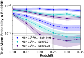
We present the efficiency curve for group 7 in Figure 4(d). The SNR of a signal is roughly inversely proportional to luminosity distance, which for the nearby universe is approximately proportional to redshift. Therefore, on the vertical axis we plot the TAP multiplied by the redshift. If the TAP is linearly correlated with the SNR, then such multiplication should remain constant. This is exactly what we observed in the blue solid line ( and spin =0.98, FAP equals 0.1). The distribution of SNR within this redshift range (0.1-0.35) roughly spans the range of 20-60, which shows good linearity between SNR and TAP in Figure 4(a). The prediction is violated to the biggest degree for the purple dashed line ( and , FAP equals 0.01). Closer events are gaining more detection efficiency, which can be expected from the non-linearity of the dashed line in the similar SNR range in Figure 4(a).
From the above analyses, we can conclude that among all factors, the SNR has the strongest influence on the expected detection efficiency. Changes in other parameters can also lead to a different performance in TAP, but such differences can be mostly explained by the different SNRs.
VI conclusions and Future works
The GW detection of EMRI signals is challenging from multiple perspectives. The accurate modeling of the EMRI waveform is a challenging task for theorists. At the same time a template bank with templates is needed, if one is to adopt the traditional matched filtering method Gair et al. (2004). In this work, we demonstrate a proof-of-principle application of a CNN on the detections of EMRIs signals. Specifically, an EMRI source with a signal-to-noise ratio uniformly drawn from 50 to 120 can be detected with a detection rate of 91% at a search false alarm probability of 1%. Meanwhile, the effectiveness of the CNN varies for different physical parameters, however, most of the difference can be explained by the influence on SNRs. EMRI systems associated with higher SNR can be expected to be detected with a higher chance.
Our work indicates that detecting EMRI signals with CNN is appealing, also for multiple reasons. For example, after being properly trained, the CNN can be applied to three months’ data, and finish the classification within one second. On the other hand, CNN shows a good generalization ability against a change of waveform models. While training on the less physical AK waveform, the network can successfully recognize signals injected with AAK waveforms. This implies that the CNN method has the potential to achieve actual detections even without accurately modeled waveforms.
It is important to benchmark the performance of the CNN to other methods. However, to the best of the authors’ knowledge, there is no other study that uses physical EMRI waveforms to search the signal and also provides a FAP estimate Wang et al. (2012). For example, some studies use physical waveforms to search for the signal, but no FAP is available Gair et al. (2004). On the other hand, other studies can provide FAP estimates, but under a very different context, and the authors adopt phenomenological waveforms for the detection Wang et al. (2012).
Although this proof-of-principle study is encouraging, we recognize that there are still lots of challenges to implement a reliable CNN to detect EMRI signals. For example, one needs to push the SNR threshold to the values lower than 50. This translates to a much larger amount of training data, the data generation, data storage, and training procedure would all become more hardware demanding. We leave the issue for future studies, with the potential of applying more sophisticated methods or constructing a hierarchical search and examining strategy for the detection pipeline.
At present, there are many Machine Learning (ML) algorithms that have wider applications in GW data analysis. For different problems in the GW field, developers use different methods or different architectures of the same method like CNN. Similar challenges might also apply to the EMRI search, and we could borrow the existing wisdom in the future.
VII Acknowledgments
The authors thank Hui-Min Fan, Lianggui Zhu, En-Kun Li, Jianwei Mei, and Micheal Williams for helpful discussions. This work has been supported by Guangdong Major Project of Basic and Applied Basic Research (Grant No. 2019B030302001), the Natural Science Foundation of China (Grants No. 12173104, No. 11805286, and No. 11690022). CM is supported by the Science and Technology Facilities Council grant ST/V005634/1. The authors would like to thank the Gravitational-wave Excellence through Alliance Training (GrEAT) network for facilitating this collaborative project. The GrEAT network is funded by the Science and Technology Facilities Council UK grant no. ST/R002770/1. NK would like to thank the support of the CNES fellowship. The authors acknowledge the uses of the calculating utilities of numpy van der Walt et al. (2011), scipy Virtanen et al. (2020), and the plotting utilities of matplotlib Hunter (2007).
References
- Abbott et al. (2019) B. P. Abbott et al. (LIGO Scientific, Virgo), Phys. Rev. X 9, 031040 (2019), arXiv:1811.12907 [astro-ph.HE] .
- Abbott et al. (2020) R. Abbott et al. (LIGO Scientific, Virgo), (2020), arXiv:2010.14527 [gr-qc] .
- Abbott et al. (2021a) R. Abbott et al. (LIGO Scientific, VIRGO), (2021a), arXiv:2108.01045 [gr-qc] .
- Abbott et al. (2021b) R. Abbott et al. (LIGO Scientific, VIRGO, KAGRA), (2021b), arXiv:2111.03606 [gr-qc] .
- Huang et al. (2020) S.-J. Huang, Y.-M. Hu, V. Korol, P.-C. Li, Z.-C. Liang, Y. Lu, H.-T. Wang, S. Yu, J. Mei, et al., Physical Review D 102, 063021 (2020).
- Korol et al. (2017) V. Korol, E. M. Rossi, P. J. Groot, G. Nelemans, S. Toonen, and A. G. A. Brown, Mon. Not. Roy. Astron. Soc. 470, 1894 (2017), arXiv:1703.02555 [astro-ph.HE] .
- Wang et al. (2019) H.-T. Wang, Z. Jiang, A. Sesana, E. Barausse, S.-J. Huang, Y.-F. Wang, W.-F. Feng, Y. Wang, Y.-M. Hu, J. Mei, et al., Physical Review D 100, 043003 (2019).
- Klein et al. (2016) A. Klein et al., Phys. Rev. D 93, 024003 (2016), arXiv:1511.05581 [gr-qc] .
- Liu et al. (2020) S. Liu, Y.-M. Hu, J.-d. Zhang, J. Mei, et al., Physical Review D 101, 103027 (2020).
- Sesana (2016) A. Sesana, Phys. Rev. Lett. 116, 231102 (2016), arXiv:1602.06951 [gr-qc] .
- Babak et al. (2017a) S. Babak, J. Gair, A. Sesana, E. Barausse, C. F. Sopuerta, C. P. Berry, E. Berti, P. Amaro-Seoane, A. Petiteau, and A. Klein, Phys. Rev. D 95, 103012 (2017a), arXiv:1703.09722 [gr-qc] .
- Fan et al. (2020) H.-M. Fan, Y.-M. Hu, E. Barausse, A. Sesana, J.-d. Zhang, X. Zhang, T.-G. Zi, and J. Mei, Phys. Rev. D 102, 063016 (2020), arXiv:2005.08212 [astro-ph.HE] .
- Liang et al. (2021) Z.-C. Liang, Y.-M. Hu, Y. Jiang, J. Cheng, J.-d. Zhang, and J. Mei, (2021), arXiv:2107.08643 [astro-ph.CO] .
- Chen et al. (2019) Z.-C. Chen, F. Huang, and Q.-G. Huang, Astrophys. J. 871, 97 (2019), arXiv:1809.10360 [gr-qc] .
- Shi et al. (2019) C. Shi, J. Bao, H.-T. Wang, J.-d. Zhang, Y.-M. Hu, A. Sesana, E. Barausse, J. Mei, J. Luo, et al., Physical Review D 100, 044036 (2019).
- Zi et al. (2021) T.-G. Zi, J.-D. Zhang, H.-M. Fan, X.-T. Zhang, Y.-M. Hu, C. Shi, and J. Mei, Phys. Rev. D 104, 064008 (2021), arXiv:2104.06047 [gr-qc] .
- Zhu et al. (2021a) L.-G. Zhu, Y.-M. Hu, H.-T. Wang, J.-D. Zhang, X.-D. Li, M. Hendry, and J. Mei, (2021a), arXiv:2104.11956 [astro-ph.CO] .
- Zhu et al. (2021b) L.-G. Zhu, L.-H. Xie, Y.-M. Hu, S. Liu, E.-K. Li, N. R. Napolitano, B.-T. Tang, J.-d. Zhang, and J. Mei, (2021b), arXiv:2110.05224 [astro-ph.CO] .
- Luo et al. (2016) J. Luo, L.-S. Chen, H.-Z. Duan, Y.-G. Gong, S. Hu, J. Ji, Q. Liu, J. Mei, V. Milyukov, M. Sazhin, et al., Classical and Quantum Gravity 33, 035010 (2016).
- Mei et al. (2020) J. Mei, Y.-Z. Bai, J. Bao, E. Barausse, L. Cai, E. Canuto, B. Cao, W.-M. Chen, Y. Chen, Y.-W. Ding, et al., Progress of Theoretical and Experimental Physics (2020).
- Baker et al. (2019) J. Baker et al., (2019), arXiv:1907.06482 [astro-ph.IM] .
- Amaro-Seoane et al. (2007) P. Amaro-Seoane, J. R. Gair, M. Freitag, M. Coleman Miller, I. Mandel, C. J. Cutler, and S. Babak, Class. Quant. Grav. 24, R113 (2007), arXiv:astro-ph/0703495 .
- Moore et al. (2017) C. J. Moore, A. J. K. Chua, and J. R. Gair, Class. Quant. Grav. 34, 195009 (2017), arXiv:1707.00712 [gr-qc] .
- Yunes et al. (2012) N. Yunes, P. Pani, and V. Cardoso, Phys. Rev. D 85, 102003 (2012), arXiv:1112.3351 [gr-qc] .
- Canizares et al. (2012) P. Canizares, J. R. Gair, and C. F. Sopuerta, Phys. Rev. D 86, 044010 (2012), arXiv:1205.1253 [gr-qc] .
- Barack and Cutler (2007) L. Barack and C. Cutler, Phys. Rev. D 75, 042003 (2007), arXiv:gr-qc/0612029 .
- Lynch et al. (2021) P. Lynch, M. van de Meent, and N. Warburton, (2021), arXiv:2112.05651 [gr-qc] .
- Isoyama et al. (2021) S. Isoyama, R. Fujita, A. J. K. Chua, H. Nakano, A. Pound, and N. Sago, (2021), arXiv:2111.05288 [gr-qc] .
- Gair et al. (2004) J. R. Gair, L. Barack, T. Creighton, C. Cutler, S. L. Larson, E. S. Phinney, and M. Vallisneri, Classical and Quantum Gravity 21, S1595 (2004).
- Wang et al. (2012) Y. Wang, Y. Shang, and S. Babak, Physical Review D 86, 104050 (2012).
- Wang et al. (2015) Y. Wang, G. Heinzel, and K. Danzmann, Physical Review D 92, 044037 (2015).
- Gair and Wen (2005) J. Gair and L. Wen, Classical and Quantum Gravity 22, S1359 (2005).
- Wen and Gair (2005) L. Wen and J. R. Gair, Classical and Quantum Gravity 22, S445 (2005).
- Gair and Jones (2007) J. Gair and G. Jones, Classical and Quantum Gravity 24, 1145 (2007).
- Gair et al. (2008a) J. R. Gair, I. Mandel, and L. Wen, Class. Quant. Grav. 25, 184031 (2008a), arXiv:0804.1084 [gr-qc] .
- Gair et al. (2008b) J. R. Gair, E. Porter, S. Babak, and L. Barack, Classical and Quantum Gravity 25, 184030 (2008b).
- Babak et al. (2009) S. Babak, J. R. Gair, and E. K. Porter, Classical and quantum gravity 26, 135004 (2009).
- Ali et al. (2012) A. Ali, N. Christensen, R. Meyer, and C. Rover, Class. Quant. Grav. 29, 145014 (2012), arXiv:1301.0455 [gr-qc] .
- Chua (2016) A. J. K. Chua, J. Phys. Conf. Ser. 716, 012028 (2016), arXiv:1602.00620 [gr-qc] .
- Chua et al. (2020) A. J. K. Chua, N. Korsakova, C. J. Moore, J. R. Gair, and S. Babak, Phys. Rev. D 101, 044027 (2020), arXiv:1912.11543 [astro-ph.IM] .
- Krizhevsky et al. (2012) A. Krizhevsky, I. Sutskever, and G. E. Hinton, Advances in neural information processing systems 25, 1097 (2012).
- Simonyan and Zisserman (2014) K. Simonyan and A. Zisserman, arXiv e-prints , arXiv:1409.1556 (2014), arXiv:1409.1556 [cs.CV] .
- Szegedy et al. (2015) C. Szegedy, V. Vanhoucke, S. Ioffe, J. Shlens, and Z. Wojna, arXiv e-prints , arXiv:1512.00567 (2015), arXiv:1512.00567 [cs.CV] .
- He et al. (2015) K. He, X. Zhang, S. Ren, and J. Sun, arXiv e-prints , arXiv:1512.03385 (2015), arXiv:1512.03385 [cs.CV] .
- Chollet (2016) F. Chollet, arXiv e-prints , arXiv:1610.02357 (2016), arXiv:1610.02357 [cs.CV] .
- Szegedy et al. (2016) C. Szegedy, S. Ioffe, V. Vanhoucke, and A. Alemi, arXiv e-prints , arXiv:1602.07261 (2016), arXiv:1602.07261 [cs.CV] .
- Deng et al. (2013) L. Deng, J. Li, J.-T. Huang, K. Yao, D. Yu, F. Seide, M. Seltzer, G. Zweig, X. He, J. Williams, Y. Gong, and A. Acero (IEEE International Conference on Acoustics, Speech, and Signal Processing (ICASSP), 2013).
- Collobert et al. (2011) R. Collobert, J. Weston, L. Bottou, M. Karlen, K. Kavukcuoglu, and P. Kuksa, arXiv e-prints , arXiv:1103.0398 (2011), arXiv:1103.0398 [cs.LG] .
- George and Huerta (2018a) D. George and E. A. Huerta, Phys. Rev. D 97, 044039 (2018a), arXiv:1701.00008 [astro-ph.IM] .
- George and Huerta (2018b) D. George and E. A. Huerta, Phys. Lett. B 778, 64 (2018b), arXiv:1711.03121 [gr-qc] .
- Huerta et al. (2019) E. Huerta, G. Allen, I. Andreoni, J. Antelis, E. Bachelet, G. Berriman, F. Bianco, R. Biswas, M. Carrasco?Kind, K. Chard, M. Cho, P. Cowperthwaite, Z. Etienne, M. Fishbach, F. Forster, D. George, T. Gibbs, M. Graham, W. Gropp, and Z. Zhao, Nature Reviews Physics 1, 1 (2019).
- Xia et al. (2020) H. Xia, L. Shao, J. Zhao, and Z. Cao, (2020), arXiv:2011.04418 [astro-ph.HE] .
- Gabbard et al. (2018) H. Gabbard, M. Williams, F. Hayes, and C. Messenger, Phys. Rev. Lett. 120, 141103 (2018), arXiv:1712.06041 [astro-ph.IM] .
- Schäfer et al. (2020) M. B. Schäfer, F. Ohme, and A. H. Nitz, Physical Review D 102, 063015 (2020).
- Krastev et al. (2021) P. G. Krastev, K. Gill, V. A. Villar, and E. Berger, Phys. Lett. B 815, 136161 (2021), arXiv:2012.13101 [astro-ph.IM] .
- Chan et al. (2020) M. L. Chan, I. S. Heng, and C. Messenger, Physical Review D 102, 043022 (2020).
- Bayley et al. (2019) J. Bayley, C. Messenger, and G. Woan, Phys. Rev. D 100, 023006 (2019).
- Bayley et al. (2020) J. Bayley, C. Messenger, and G. Woan, Phys. Rev. D 102, 083024 (2020).
- Gabbard et al. (2019) H. Gabbard, C. Messenger, I. S. Heng, F. Tonolini, and R. Murray-Smith, (2019), arXiv:1909.06296 [astro-ph.IM] .
- Williams et al. (2021) M. J. Williams, J. Veitch, and C. Messenger, (2021), arXiv:2102.11056 [gr-qc] .
- George et al. (2017) D. George, H. Shen, and E. A. Huerta, in NiPS Summer School 2017 (2017) arXiv:1711.07468 [astro-ph.IM] .
- Shen et al. (2019) H. Shen, D. George, E. A. Huerta, and Z. Zhao, (2019), 10.1109/ICASSP.2019.8683061, arXiv:1903.03105 [astro-ph.CO] .
- Heaton (2017) J. Heaton, Genetic Programming and Evolvable Machines 19 (2017), 10.1007/s10710-017-9314-z.
- Amaro-Seoane (2018) P. Amaro-Seoane, Living Rev. Rel. 21, 4 (2018), arXiv:1205.5240 [astro-ph.CO] .
- Pan and Yang (2021) Z. Pan and H. Yang, Phys. Rev. D 103, 103018 (2021), arXiv:2101.09146 [astro-ph.HE] .
- Pan et al. (2021) Z. Pan, Z. Lyu, and H. Yang, Phys. Rev. D 104, 063007 (2021), arXiv:2104.01208 [astro-ph.HE] .
- Arcodia et al. (2021) R. Arcodia et al., Nature 592, 704 (2021), arXiv:2104.13388 [astro-ph.HE] .
- Babak et al. (2017b) S. Babak, J. Gair, A. Sesana, E. Barausse, C. F. Sopuerta, C. P. Berry, E. Berti, P. Amaro-Seoane, A. Petiteau, and A. Klein, Physical Review D 95, 103012 (2017b).
- Barack (2009) L. Barack, Classical and Quantum Gravity 26, 213001 (2009).
- Van De Meent (2018) M. Van De Meent, Physical Review D 97, 104033 (2018).
- Miller and Pound (2021) J. Miller and A. Pound, Phys. Rev. D 103, 064048 (2021), arXiv:2006.11263 [gr-qc] .
- Hughes et al. (2021) S. A. Hughes, N. Warburton, G. Khanna, A. J. K. Chua, and M. L. Katz, Phys. Rev. D 103, 104014 (2021), arXiv:2102.02713 [gr-qc] .
- McCart et al. (2021) J. McCart, T. Osburn, and J. Y. J. Burton, Phys. Rev. D 104, 084050 (2021), arXiv:2109.00056 [gr-qc] .
- Hughes et al. (2005) S. A. Hughes, S. Drasco, E. E. Flanagan, and J. Franklin, Physical review letters 94, 221101 (2005).
- Babak et al. (2007) S. Babak, H. Fang, J. R. Gair, K. Glampedakis, and S. A. Hughes, Physical Review D 75, 024005 (2007).
- Barack and Cutler (2004) L. Barack and C. Cutler, Phys. Rev. D 69, 082005 (2004), arXiv:gr-qc/0310125 [gr-qc] .
- Chua and Gair (2015a) A. J. Chua and J. R. Gair, Classical and Quantum Gravity 32, 232002 (2015a).
- Katz et al. (2021) M. L. Katz, A. J. K. Chua, L. Speri, N. Warburton, and S. A. Hughes, Phys. Rev. D 104, 064047 (2021), arXiv:2104.04582 [gr-qc] .
- Chua and Gair (2015b) A. J. K. Chua and J. R. Gair, Class. Quant. Grav. 32, 232002 (2015b), arXiv:1510.06245 [gr-qc] .
- Cutler (1998) C. Cutler, Physical Review D 57, 7089 (1998).
- Cornish and Larson (2001) N. J. Cornish and S. L. Larson, Classical and Quantum Gravity 18, 3473 (2001).
- Cornish and Rubbo (2003) N. J. Cornish and L. J. Rubbo, Physical Review D 67, 022001 (2003).
- Zhang et al. (2020) C. Zhang, Q. Gao, Y. Gong, B. Wang, A. J. Weinstein, C. Zhang, et al., Physical Review D 101, 124027 (2020).
- Estabrook et al. (2000) F. B. Estabrook, M. Tinto, and J. W. Armstrong, Phys. Rev. D 62, 042002 (2000).
- Tinto and Armstrong (1999) M. Tinto and J. W. Armstrong, Phys. Rev. D 59, 102003 (1999).
- Ng et al. (2013) A. Ng, J. Ngiam, C. Y. Foo, Y. Mai, C. Suen, A. Coates, A. Maas, A. Hannun, B. Huval, T. Wang, et al., “Unsupervised feature learning and deep learning,” (2013).
- LeCun et al. (2015) Y. LeCun et al., URL: http://yann. lecun. com/exdb/lenet 20, 14 (2015).
- Dozat (2016) T. Dozat, (2016).
- Yao (2007) Y. L. R. A. C. Yao, Constructive Approximation. 26, 289 (2007).
- van der Walt et al. (2011) S. van der Walt, S. C. Colbert, and G. Varoquaux, Comput. Sci. Eng. 13, 22 (2011), arXiv:1102.1523 [cs.MS] .
- Virtanen et al. (2020) P. Virtanen et al., Nature Meth. 17, 261 (2020), arXiv:1907.10121 [cs.MS] .
- Hunter (2007) J. D. Hunter, Comput. Sci. Eng. 9, 90 (2007).