Detailed fluctuation theorem from the one-time measurement scheme

Kenji Maeda Department of Physics, University of Massachusetts, Boston, Massachusetts 02125, USA Tharon Holdsworth Department of Physics, University of Massachusetts, Boston, Massachusetts 02125, USA Sebastian Deffner Department of Physics, University of Maryland, Baltimore County, Baltimore, Maryland 21250, USA Akira Sone [email protected] Department of Physics, University of Massachusetts, Boston, Massachusetts 02125, USA

Abstract

We study the quantum fluctuation theorem in the one-time measurement (OTM) scheme, where the work distribution of the backward process has been lacking and which is considered to be more informative than the two-time measurement (TTM) scheme. We find that the OTM scheme is the quantum nondemolition TTM scheme, in which the final state is a pointer state of the second measurement whose Hamiltonian is conditioned on the first measurement outcome. Then, by clarifying the backward work distribution in the OTM scheme, we derive the detailed fluctuation theorem in the OTM scheme for the characteristic functions of the forward and backward work distributions, which captures the detailed information about the irreversibility and can be applied to quantum thermometry. We also verified our conceptual findings with the IBM quantum computer. Our result clarifies that the laws of thermodynamics at the nanoscale are dependent on the choice of the measurement and may provide experimentalists with a concrete strategy to explore laws of thermodynamics at the nanoscale by protecting quantum coherence and correlations.

One of the most significant conceptual factors distinguishing quantum physics and classical physics is measurement [1]. In quantum mechanics, measurements typically destroy quantum coherences and correlations that could be utilized as the resources for many quantum engineering tasks, such as quantum computing and quantum metrology. Compared to classical systems, one has many degrees of freedom in choosing the basis of the measurement based on their task on the quantum system. Particularly, the eigenbasis of the observable of the measurement apparatus is comprised of the so-called pointer states [2, 3, 4, 5, 6], which are immune to decoherence due to the corresponding measurement.

Quantum thermodynamics [7, 8, 9] is a rapidly growing field exploring the laws of thermodynamics from the perspective of quantum information science. Fluctuation theorems [10, 11] in both quantum and classical systems are regarded as one of the most significant laws to date [12] because many significant thermodynamic principles can be derived, such as the second law of thermodynamics [13] and response theory [14, 15]. The standard approach toward quantum fluctuation theorem is the so-called two-time measurement (TTM) scheme [16, 17, 18, 19, 20, 21, 22, 23, 24, 25, 26, 27, 28, 29, 30, 31].

The TTM scheme is constructed by two energy projection measurements at the beginning and the end of a quantum process. In the standard setup of the time-varying Hamiltonian system, the initial state is prepared in the Gibbs state defined by its initial Hamiltonian $H_{0}$ . Then, one performs an energy measurement on the initial state with $H_{0}$ , which projects the system onto one of the eigenstates $|E_{i}\rangle$ of $H_{0}$ based on the initial measurement outcome $E_{i}$ . Then, one evolves the system under the unitary operator $U$ during time $\tau$ and measures the evolved state $U|E_{i}\rangle$ with the final Hamiltonian $H_{\tau}$ . Finally, the system will be projected again onto an eigenstate $|E_{j}^{\prime}\rangle$ of $H_{\tau}$ based on the final measurement outcome $E_{j}^{\prime}$ .

The work performed on the system in a single realization is defined by the difference between the final and initial measurement outcome, $W_{i\to j}\equiv E_{j}^{\prime}-E_{i}$ , which recovers the standard fluctuation theorem, also known as the TTM fluctuation theorem resembling the classical Jarzynksi equality [10]. Therefore, the TTM scheme can be regarded as a semiclassical approach, which has been experimentally implemented in various systems [32, 33, 34, 35, 36, 37, 38, 39, 40, 41, 42], including a demonstration on the DWave machine [30]. However, the second projection measurement usually destroys the quantum coherence and correlations generated through the dynamics, which means that the TTM cannot fully capture the peculiar features of the quantum systems when one analyzes its thermodynamic behaviors [29].

To address the thermodynamic contribution of quantum correlations, Ref. [43] proposed the so-called one-time measurement (OTM) scheme. In this scheme, the second measurement is considered to be avoided, and the work is determined by the energy difference conditioned on the initial energy measurement outcome. Within this paradigm, the corresponding Jarzynski equality includes the additional information contribution stemming from the quantum relative entropy of the conditional thermal state [44, 45] with respect to the Gibbs state defined by the final Hamiltonian. This additional term provides a tighter maximum work relation and captures the quantum coherence or correlations generated through the dynamics in the formalism. Therefore, the OTM scheme can be regarded as more informative than the TTM scheme. This has been elucidated in various contexts, including quantum thermometry [45], work as an external quantum observable [46], distinguishability of heat and work in an open quantum system [47], heat exchange [48], classical correspondence of the OTM scheme [44], quantum ergotropy [49], and information production [50]. However, the backward process in the OTM scheme has not been considered yet, which has made the detailed quantum fluctuation theorem of the OTM scheme elusive.

In the present Letter, we first prove that the OTM scheme is the quantum nondemolition (QND) TTM scheme, where the pointer states of the second measurement (conditional Hamiltonian) are the evolved states conditioned on the initial measurement outcome. From this, we construct the backward work distribution and derive the detailed quantum fluctuation theorem of the OTM scheme, which we call OTM fluctuation theorem. Then, we propose a quantum circuit to compute the symmetric relation of the characteristic functions of the forward and backward work distributions. We explore the physical meaning of the OTM fluctuation theorem by associating it to the concept of irreversibility and demonstrate the potential application of the derived formalism to state preparation for low-temperature quantum thermometry. Finally, we verify the derived detailed fluctuation theorem with IBM quantum computer to demonstrate the experimental implementability of the OTM scheme. These results emphasize that the laws of quantum thermodynamics are strictly determined by the choice of measurements by the observers.

OTM detailed fluctuation theorem

Our first result is the derivation of the OTM fluctuation theorem. We consider a finite-dimensional closed quantum system described by a $d$ -dimensional Hilbert space. Let the initial state be a Gibbs state $\rho_{0}^{\text{eq}}\equiv\exp(-\beta H_{0})/Z_{0}$ , where $H_{0}$ is the initial Hamiltonian and $Z_{0}\equiv\mathrm{tr}\left\{\exp(-\beta H_{0})\right\}$ is the partition function. In a closed quantum system, the time evolution is described by a unitary operator $U$ . In the OTM scheme, the work for a single realization of the protocol is defined as

\widetilde{W}_{i}\equiv\langle E_{i}\hskip 1.0pt|U^{\dagger}H_{\tau}U|\hskip 1.0ptE_{i}\rangle-E_{i},

(1)

which also has been called conditional work [44]. This is the energy difference between the final energy conditioned on the initial measurement outcome and itself. Then, the forward conditional work distribution is simply given by [43]

\widetilde{P}_{f}(W)=\sum_{i=1}^{d}\frac{e^{-\beta E_{i}}}{Z_{0}}\delta\left(W-\widetilde{W}_{i}\right),

(2)

which is consistent with the exact average work

\langle W\rangle=\int W\widetilde{P}_{f}(W)dW=\mathrm{tr}\left\{\left(U^{\dagger}H_{\tau}U-H_{0}\right)\rho_{0}^{\text{eq}}\right\}

(3)

and yields the generalized Jarzynski equality [43]

\langle e^{-\beta W}\rangle_{\widetilde{P}}=\frac{\widetilde{Z}_{\tau}}{Z_{0}}=e^{-\beta\Delta F}e^{-S(\widetilde{\rho}_{\tau}||\rho_{\tau}^{\text{eq}})}.

(4)

In Eq. (4), the conditional partition function, $\widetilde{Z}_{\tau}\equiv\sum_{i=1}^{d}\exp{\left(-\beta\langle E_{i}\hskip 1.0pt|U^{\dagger}H_{\tau}U|\hskip 1.0ptE_{i}\rangle\right)}$ , is the normalization factor used to construct the conditional thermal state,

\widetilde{\rho}_{\tau}\equiv\sum_{i=1}^{d}\frac{e^{-\beta\langle E_{i}\hskip 1.0pt|U^{\dagger}H_{\tau}U|\hskip 1.0ptE_{i}\rangle}}{\widetilde{Z}_{\tau}}U|E_{i}\rangle\!\langle E_{i}|U^{\dagger}.

(5)

Finally, $S(\widetilde{\rho}_{\tau}||\rho_{\tau}^{\text{eq}})=\mathrm{tr}\left\{\widetilde{\rho}_{\tau}\ln\widetilde{\rho}_{\tau}\right\}-\mathrm{tr}\left\{\widetilde{\rho}_{\tau}\ln\rho_{\tau}^{\text{eq}}\right\}$ is the quantum relative entropy of the conditional thermal state with respect to the Gibbs state $\rho_{\tau}^{\text{eq}}\equiv\exp(-\beta H_{\tau})/Z_{\tau}$ of the final Hamiltonian $H_{\tau}$ .

By comparing with the TTM scheme, we demonstrate that the OTM scheme is equivalent to the TTM scheme with a carefully chosen final Hamiltonian (conditional Hamiltonian) based on the information about the initial measurement outcome and the dynamics of the system. To see this point, let us define the conditional Hamiltonian $G_{\tau}$ ,

G_{\tau}\equiv\sum_{i=1}^{d}\langle E_{i}\hskip 1.0pt|U^{\dagger}H_{\tau}U|\hskip 1.0ptE_{i}\rangle U|E_{i}\rangle\!\langle E_{i}|U^{\dagger},

(6)

where $E_{i}$ is the eigenenergy of the initial Hamiltonian $H_{0}$ with its corresponding eigenstate $|E_{i}\rangle$ . At $t=0$ we perform a projective energy measurement $H_{0}$ on the system initially prepared in $\rho_{0}^{\text{eq}}$ . Then, the post-measurement state will be projected onto $|E_{i}\rangle$ with the corresponding energy $E_{i}$ . After the evolution, the state is $U|E_{i}\rangle$ . At $t=\tau$ we perform the second measurement $G_{\tau}$ . Since the final state is a pointer state of $G_{\tau}$ , it is not destroyed by the measurement, so that the observer obtains the final energy measurement outcome $\langle E_{i}\hskip 1.0pt|U^{\dagger}H_{\tau}U|\hskip 1.0ptE_{i}\rangle$ , while the system remains as $U|E_{i}\rangle$ . The corresponding quantum work is simply given by Eq. (1).

Then, the equivalent work distribution within the TTM paradigm, the forward work distribution is computed as

\widetilde{P}_{f}(W)=\sum_{i=1}^{d}\frac{e^{-\beta\langle E_{i}\hskip 1.0pt|H_{0}|\hskip 1.0ptE_{i}\rangle}}{Z_{0}}|\langle E_{i}\hskip 1.0pt|U^{\dagger}U|\hskip 1.0ptE_{i}\rangle|^{2}\delta(W-\widetilde{W}_{i}),

(7)

which is identical to Eq. (2).

This is our first main result, namely we have that the OTM scheme is exactly the QND TTM scheme, in which the second projection measurement does not destroy the evolved state conditioned on the initial measurement outcome (see Fig. 1 and [51]). We will now exploit this insight to construct the conditional work distribution for the backward process within the OTM paradigm.

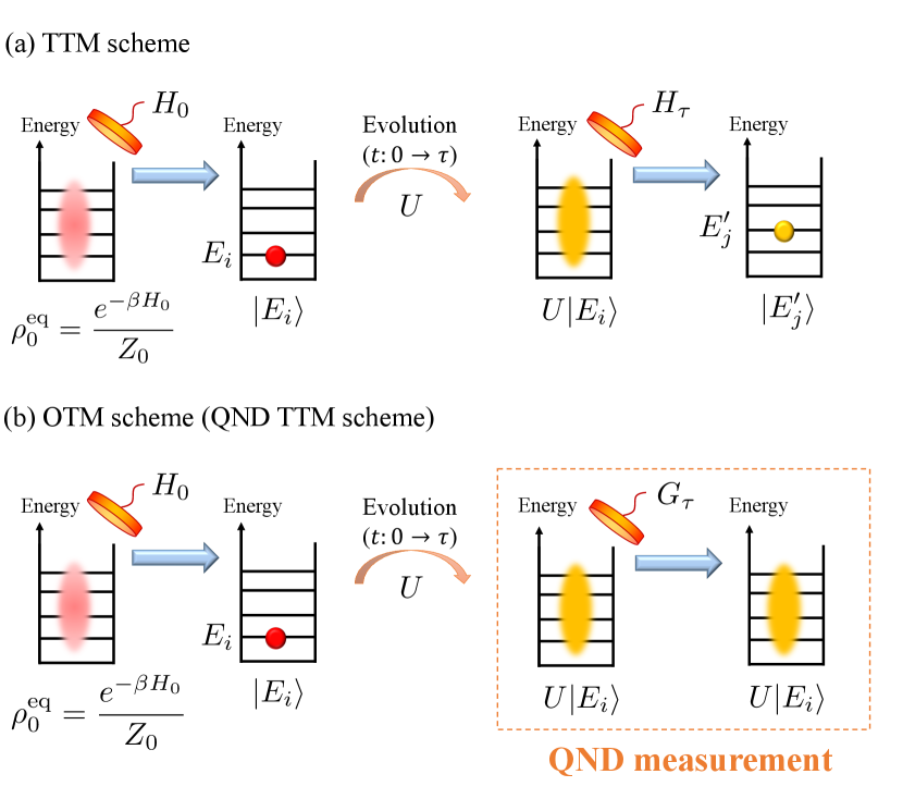
Refer to caption — Figure 1: Comparison between the TTM and OTM scheme. In (a) the standard TTM scheme, in which the second energy measurement is the final Hamiltonian, the projection measurement projects the evolved state $U|E_{i}\rangle$ onto $|E_{j}^{\prime}\rangle$ the eigenstate of $H_{\tau}$ . In (b) the OTM scheme, the final Hamiltonian $G_{\tau}\equiv\sum_{i=1}^{d}\langle E_{i}\hskip 1.0pt|U^{\dagger}H_{\tau}U|\hskip 1.0ptE_{i}\rangle U|E_{i}\rangle\!\langle E_{i}|U^{\dagger}$ is the conditional Hamiltonian with its pointer state $U|E_{i}\rangle$ , which is equivalent to the evolved state conditioned on the initial measurement outcome. Therefore, this measurement preserves the state $U|E_{i}\rangle$ . In this sense, this measurement is a QND measurement.

The backward process is initialized from the state $\widetilde{\rho}_{\tau}\equiv{\exp{\left(-\beta G_{\tau}\right)}}/{\widetilde{Z}_{\tau}}$ . After the backward evolution described by $U^{\dagger}$ , the measurement $H_{0}$ is performed on the final state of the backward process. Since the final state is $U^{\dagger}U|E_{i}\rangle=|E_{i}\rangle$ , which is a pointer state of $H_{0}$ , $H_{0}$ does not destroy the state. Moreover, the outcome is always $E_{i}$ .

Then, by following the TTM scheme, the conditional work distribution of the backward process is given by

\widetilde{P}_{b}(-W)\equiv\sum_{i=1}^{d}\frac{e^{-\beta\langle E_{i}\hskip 1.0pt|U^{\dagger}H_{\tau}U|\hskip 1.0ptE_{i}\rangle}}{\widetilde{Z}_{\tau}}\delta(-W+\widetilde{W}_{i}).

(8)

From Eq. (8) we now derive the fluctuation theorem [52, 53, 54] between the forward conditional work distribution and backward distribution in the characteristic function form.

The characteristic functions are defined as the Fourier transform of the work distributions

\begin{split}\widetilde{C}_{f}(u)&\equiv\int dW\widetilde{P}_{f}(W)e^{iuW}\\ \widetilde{C}_{b}(u)&\equiv\int dW\widetilde{P}_{b}(-W)e^{-iuW}.\end{split}

(9)

By applying the approach to the TTM scheme in Ref. [52, 53, 54], the characteristic functions are equivalent to

\begin{split}\widetilde{C}_{f}(u)&=\mathrm{tr}\left\{U^{\dagger}e^{iuG_{\tau}}Ue^{-iuH_{0}}\rho^{\text{eq}}_{0}\right\}\\ \widetilde{C}_{b}(u)&=\mathrm{tr}\left\{Ue^{iuH_{0}}U^{\dagger}e^{-iuG_{\tau}}\widetilde{\rho}_{\tau}\right\}.\end{split}

(10)

Thus, we obtain the following symmetry relation ¹¹1In Supplemental Material [51], we provide the proof for the case that the initial state is also the conditional thermal state defined by $G_{0}\equiv\sum_{i=1}^{d}\langle\psi_{i}\hskip 1.0pt|H_{0}|\hskip 1.0pt\psi_{i}\rangle|\psi_{i}\rangle\!\langle\psi_{i}|$ with $|\psi_{i}\rangle$ being not necessarily the eigenstate of $H_{0}$ . Equation. (11) can be regarded as its corollary. , which is our second main result,

\frac{\widetilde{C}_{f}(u)}{\widetilde{C}_{b}(-u+i\beta)}=\frac{\widetilde{Z}_{\tau}}{Z_{0}}=e^{-\beta\Delta F-S(\widetilde{\rho}_{\tau}||\rho_{\tau}^{\text{eq}})},

(11)

where

\widetilde{C}_{b}(-u+i\beta)=\mathrm{tr}\left\{Ue^{-iuH_{0}}e^{-\beta H_{0}}U^{\dagger}e^{iuG_{\tau}}e^{\beta G_{\tau}}\widetilde{\rho}_{\tau}\right\}.

(12)

The characteristic functions can be determined directly from quantum circuits, and hence our results permit the demonstration of the experimental implementability of the OTM scheme in the single qubit interferometry.

Single-qubit interferometry approach.

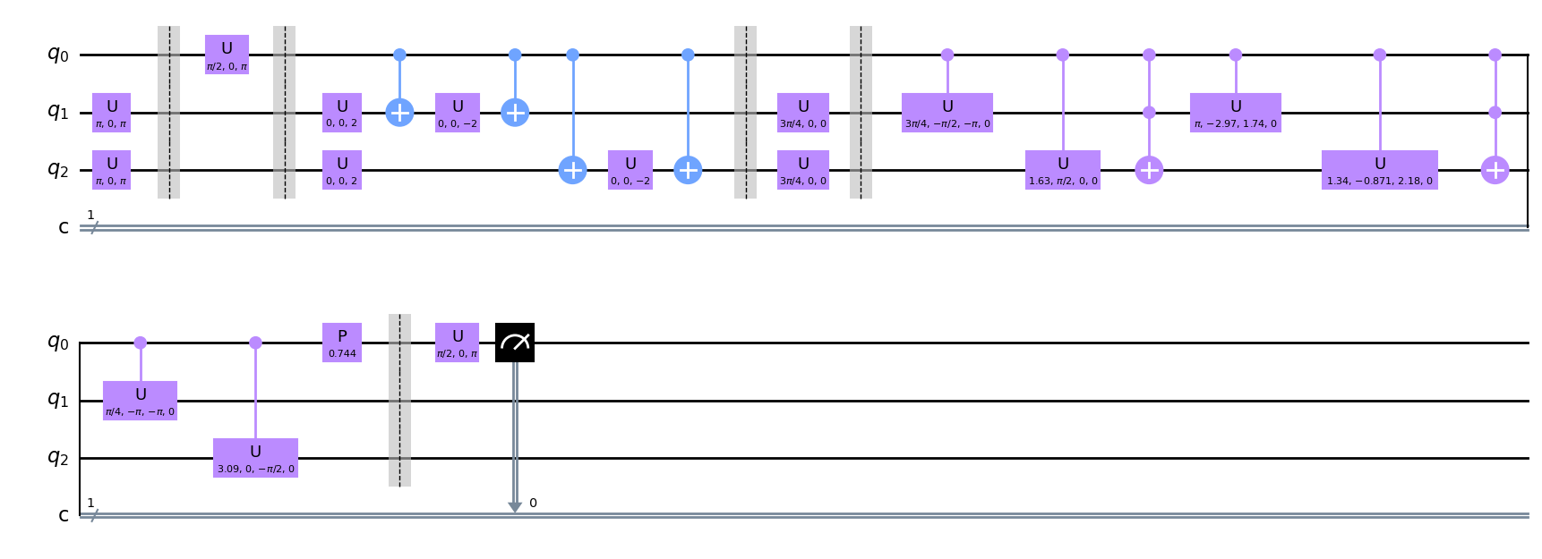
By employing the single-qubit interferometry approach developed in Refs. [53, 54], we now construct a quantum algorithm to verify Eq. (11). This indicates that the OTM scheme is experimentally implementable, which is our third main result.

Let us define $|0\rangle\equiv\begin{pmatrix}1&0\end{pmatrix}^{T}$ and $|1\rangle\equiv\begin{pmatrix}0&1\end{pmatrix}^{T}$ . We denote by $\openone$ the $2\times 2$ identity matrix and $X$ , $Y$ , $Z$ as the usual Pauli matrices. Also, we write the Hadamard gate as $\mathbf{H}\equiv\frac{1}{\sqrt{2}}\begin{pmatrix}1&1\\ 1&-1\end{pmatrix}$ . Then, the characteristic function of the forward process $\widetilde{C}_{f}(u)$ can be computed by the quantum circuit depicted in Fig. 2. In this circuit, the ancilla qubit is initially prepared in $|0\rangle$ . The target system is prepared in the Gibbs state $\rho_{0}^{\text{eq}}$ . To obtain the characteristic function $\widetilde{C}_{f}(u)$ , we measure the output state of the ancilla qubit with $X$ and $Y$ , whose expectation values become $\langle X\rangle=\text{Re}[\widetilde{C}_{f}(u)]$ and $\langle Y\rangle=\text{Im}[\widetilde{C}_{f}(u)]$ .

\Qcircuit@C=1em @R=1.2em \lstick|0⟩& \gateH \ctrl0 \qwx[1] \qw \ctrl0 \qwx[1] \meter $X$ , $Y$
\lstickρ_0^eq\qw \gatee^-i u H_0 \gateU \gatee^iu G_τ \qw

Figure 2: Quantum circuit for computing

\widetilde{C}_{f}(u)

. The expectation values of

X

and

Y

obtained by measuring the final state of the ancilla qubit are

\text{Re}[\widetilde{C}_{f}(u)]

and

\text{Im}[\widetilde{C}_{f}(u)]

, respectively.

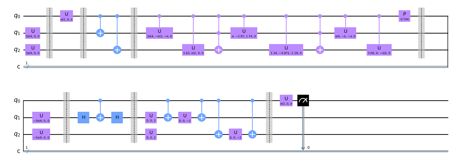
Next, we consider the quantum circuit to compute the characteristic function of the backward process $\widetilde{C}_{b}(-u+i\beta)$ . From Eq. (12), we need to first decompose $\exp(\beta G_{\tau})$ and $\exp(-\beta H_{0})$ with Pauli string $\{\sigma_{k}\}_{k=1}^{d^{2}}$ , where $\sigma_{1}$ is the $d\times d$ identity matrix ²²2When $d=4$ , the Pauli string is $\{\openone,X\otimes\openone,Y\otimes\openone,Z\otimes\openone,\openone\otimes X,\openone\otimes Y,\openone\otimes Z,X\otimes X,X\otimes Y,X\otimes Z,Y\otimes X,Y\otimes Y,Y\otimes Z,Z\otimes X,Z\otimes Y,Z\otimes Z\}$ , which has $4^{2}=16$ elements, and these elements are the bases constructing any $4\times 4$ matrix.. Here, note that $\frac{1}{d}\mathrm{tr}\left\{\sigma_{k}\sigma_{\ell}\right\}=\delta_{k\ell}$ becomes Kronecker’s delta. Then, we can write $\exp(-\beta H_{0})=\sum_{k=1}^{d^{2}}\alpha_{k}^{(0)}\sigma_{k}$ and $\exp(\beta G_{\tau})=\sum_{k=1}^{d^{2}}\alpha_{k}^{(\tau)}\sigma_{k}$ , where $\alpha_{k}^{(0)}=\frac{1}{d}\mathrm{tr}\left\{e^{-\beta H_{0}}\sigma_{k}\right\}$ and $\alpha_{k}^{(\tau)}=\frac{1}{d}\mathrm{tr}\left\{e^{\beta G_{\tau}}\sigma_{k}\right\}$ . Note that the coefficients $\{\alpha_{k}^{(0)},\alpha_{k}^{(\tau)}\}_{k=1}^{d^{2}}$ are computable via a classical computer since we have full knowledge of $H_{0}$ , $H_{\tau}$ , and $U$ if $d$ is smaller. Therefore, we can write

\widetilde{C}_{b}(-u+i\beta)=\sum_{k,\ell}\alpha_{k}^{(0)}\alpha_{\ell}^{(\tau)}F_{k\ell},

(13)

where we define

F_{k\ell}\equiv\mathrm{tr}\left\{U\sigma_{k}e^{-iuH_{0}}U^{\dagger}\sigma_{\ell}e^{iuG_{\tau}}\widetilde{\rho}_{\tau}\right\}.

(14)

Then, we can employ the quantum circuit depicted in Fig. 3 to compute $F_{k\ell}$ . In this circuit, the ancilla qubit is prepared in $|0\rangle$ . The target system is prepared in the conditional thermal state $\widetilde{\rho}_{\tau}$ . Here, the expectation values become $\langle X\rangle=\text{Re}[F_{k\ell}]$ and $\langle Y\rangle=\text{Im}[F_{k\ell}]$ . Given the fact that we have already known $\{\alpha_{k}^{(0)},\alpha_{k}^{(\tau)}\}_{k=1}^{d^{2}}$ via a classical computer, from Eq. (13), we can finally obtain $\widetilde{C}_{b}(-u+i\beta)$ .

\Qcircuit@C=1em @R=1.2em \lstick|0⟩& \gateH \ctrl0 \qwx[1] \ctrl0 \qwx[1] \qw \ctrl0 \qwx[1] \ctrl0 \qwx[1] \meter $X$ , $Y$
\lstick~ρ_τ\qw \gatee^iu G_τ\gateσ_ℓ \gateU^† \gatee^-iuH_0 \gateσ_k \qw

Figure 3: Quantum circuit for computing

F_{k\ell}

: The expectation values of

X

and

Y

obtained by measuring the final state of the ancilla qubit are

\text{Re}[F_{k\ell}]

and

\text{Im}[F_{k\ell}]

, respectively.

Physical meaning of OTM fluctuation theorem.

By considering the backward process, we can find that the OTM fluctuation theorem can capture the detailed information about the irreversibility and be applied to state preparation for quantum thermometry in the low-temperature limit. To quantify the irreversibility of a quantum process, we consider the Kullback-Leibler (KL) divergence $D[\widetilde{P}_{f}||\widetilde{P}_{b}]$ of $\widetilde{P}_{f}(W)$ with respect to $\widetilde{P}_{b}(-W)$ , which is defined as

\displaystyle D[\widetilde{P}_{f}||\widetilde{P}_{b}]\equiv\int dW\widetilde{P}_{f}(W)\ln\left(\frac{\widetilde{P}_{f}(W)}{\widetilde{P}_{b}(-W)}\right).

(15)

From Eqs. (2) and (8), we obtain [51]

\displaystyle\!\!\!\!D[\widetilde{P}_{f}||\widetilde{P}_{b}]\!=\!-S(\rho_{0}^{\text{eq}})+\beta\mathrm{tr}\left\{U\rho_{0}^{\text{eq}}U^{\dagger}H_{\tau}\right\}+\ln\widetilde{Z}_{\tau},

(16)

where $S(\rho_{0}^{\text{eq}})\equiv-\mathrm{tr}\left\{\rho_{0}^{\text{eq}}\ln\rho_{0}^{\text{eq}}\right\}$ is the von-Neumann entropy of $\rho_{0}^{\text{eq}}$ . Given that the exact averaged work $\langle W\rangle\equiv\mathrm{tr}\left\{U\rho_{0}^{\text{eq}}U^{\dagger}H_{\tau}\right\}-\mathrm{tr}\left\{\rho_{0}^{\text{eq}}H_{0}\right\}$ , from Eq. (11), the excess work $\langle W_{\text{ex}}\rangle\equiv\langle W\rangle-\Delta F$ can be written as

\displaystyle\beta\langle W_{\text{ex}}\rangle=D[\widetilde{P}_{f}||\widetilde{P}_{b}]+S(\widetilde{\rho}_{\tau}||\rho_{\tau}^{\text{eq}}).

(17)

This means that the excess work $\langle W_{\text{ex}}\rangle$ is a sum of the KL divergence $D[\widetilde{P}_{f}||\widetilde{P}_{b}]$ , which characterizes the irreversible process, and $\beta S(\widetilde{\rho}_{\tau}||\rho_{\tau}^{\text{eq}})$ , which is the energy dissipated into the heat bath when the system is thermalized from $\widetilde{\rho}_{\tau}$ . Therefore, $\beta S(\widetilde{\rho}_{\tau}||\rho_{\tau}^{\text{eq}})$ can be interpreted as a heatlike quantity.

Furthermore, $D[\widetilde{P}_{f}||\widetilde{P}_{b}]$ can be employed in quantum thermometry in the low-temperature limit. In Ref. [45], it was demonstrated that the conditional thermal state $\widetilde{\rho}_{\tau}$ can outperform the Gibbs state $\rho_{\tau}^{\text{eq}}$ in the low-temperature limit. Therefore, preparing $\widetilde{\rho}_{\tau}$ is a desired task for quantum thermometry. First the excess work can be written as $\beta\langle W_{\text{ex}}\rangle=S(U\rho_{0}^{\text{eq}}U^{\dagger}||\rho_{\tau}^{\text{eq}})$ [57, 58, 59]. In Ref. [45], we derived the so-called thermodynamic triangle equality $S(U\rho_{0}^{\text{eq}}U^{\dagger}||\widetilde{\rho}_{\tau})+S(\widetilde{\rho}_{\tau}||\rho_{\tau}^{\text{eq}})=S(U\rho_{0}^{\text{eq}}U^{\dagger}||\rho_{\tau}^{\text{eq}})$ . Therefore, from Eq. (17), we obtain

\displaystyle D[\widetilde{P}_{f}||\widetilde{P}_{b}]=S(U\rho_{0}^{\text{eq}}U^{\dagger}||\widetilde{\rho}_{\tau}),

(18)

which measures the distinguishability of the exact final state $U\rho_{0}^{\text{eq}}U^{\dagger}$ and the conditional thermal state $\widetilde{\rho}_{\tau}$ . This quantity can be used to design the unitary process $U$ that minimizes $S(U\rho_{0}^{\text{eq}}U^{\dagger}||\widetilde{\rho}_{\tau})$ for the final exact state $U\rho_{0}^{\text{eq}}U^{\dagger}$ to be closer to $\widetilde{\rho}_{\tau}$ . Also, note that the distinguishability measure $S(U\rho_{0}^{\text{eq}}U^{\dagger}||\widetilde{\rho}_{\tau})$ can be computed by a quantum computer. From Eqs. (11) and (16), we have

\displaystyle D[\widetilde{P}_{f}||\widetilde{P}_{b}]=\beta\langle W\rangle+\ln\left(\frac{\widetilde{C}_{f}(u)}{\widetilde{C}_{b}(-u+i\beta)}\right),

(19)

where $\langle W\rangle$ , $\widetilde{C}_{f}(u)$ , and $\widetilde{C}_{b}(-u+i\beta)$ can be computed by a quantum computer.

Finally, we emphasize that these analyses are hard to conduct within the TTM scheme [31]. Therefore, our detailed fluctuation demonstrates an additional advantage of the OTM scheme.

Verification with IBM quantum computers

To conclude our analysis, we employ the IBM cloud-based quantum computer [60] to verify the detailed fluctuation theorem (11). Our setup is the following. The initial Hamiltonian $H_{0}$ is $H_{0}=\omega(Z\otimes\openone+\openone\otimes Z)$ with the corresponding eigenbasis $|E_{1}\rangle=\begin{pmatrix}1&0&0&0\end{pmatrix}^{T}$ , $|E_{2}\rangle=\begin{pmatrix}0&1&0&0\end{pmatrix}^{T}$ , $|E_{3}\rangle=\begin{pmatrix}0&0&1&0\end{pmatrix}^{T}$ , and $|E_{4}\rangle=\begin{pmatrix}0&0&0&1\end{pmatrix}^{T}$ . The final Hamiltonian is set to be $H_{\tau}=J(X\otimes X)$ . The unitary operator that describes the evolution is set as $U=\exp\left(-i\frac{\Omega\tau}{2}(Y\otimes\openone+\openone\otimes Y)\right)$ .

For the initial Gibbs state preparation, we consider the decomposition of the input mixed state. This is because we can only prepare pure states on the IBM quantum computers and $\{|E_{i}\rangle\}_{i=1}^{4}$ can be prepared. For the weights $\{\exp(-\beta E_{i})/Z_{0}\}_{i=1}^{4}$ , since we already know the initial Hamiltonian $H_{0}$ , we assume that the weights are also known and we can compute $\widetilde{C}_{f}(u)$ .

For the backward process, we need to prepare the conditional thermal state $\widetilde{\rho}_{\tau}$ as the initial state. In our simulation, we suppose that we already know $U$ ; therefore, we can prepare $\{U|E_{i}\rangle\}_{i=1}^{4}$ with the quantum computer. Similarly, because we assume that $U$ , $H_{0}$ and $H_{\tau}$ are known, the weights $\{\exp\left(-\beta\langle E_{i}\hskip 1.0pt|U^{\dagger}H_{\tau}U|\hskip 1.0ptE_{i}\rangle\right)/\widetilde{Z}_{\tau}\}_{i=1}^{4}$ are considered to be also known, which we use to compute $F_{k\ell}$ . Thus the coefficients $\alpha_{k}^{(0)}$ and $\alpha_{\ell}^{(\tau)}$ are also regarded as known values, which enables one to compute $\widetilde{C}_{b}(-u+i\beta)$ .

By setting the parameters as $\beta=0.5$ , $\omega=2$ , $\Omega=3$ , $J=1$ , and $\tau=\pi/4$ , we obtain the theoretical value of the ratio

R_{\text{true}}\equiv\frac{\widetilde{C}_{f}(u)}{\widetilde{C}_{b}(-u+i\beta)}=0.433167

(20)

for any $u$ . Here, we particularly focus on the case $u=1$ , and verify Eq. (20) with the IBM cloud-based quantum computer [60].

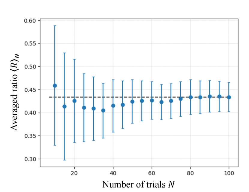
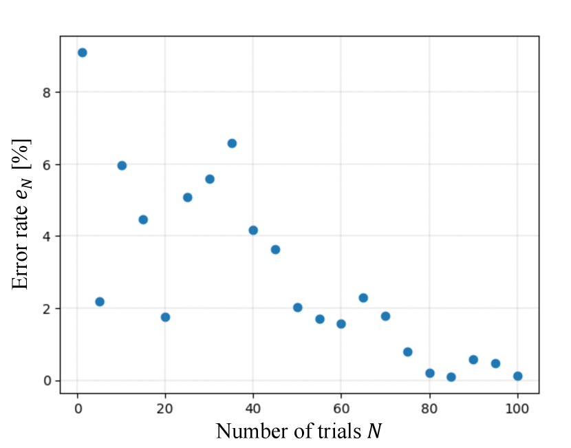
To determine $\langle X\rangle$ and $\langle Y\rangle$ , for each quantum circuit in Figs. 2 and 3, we perform the single-shot measurement $20000$ times. The median of the errors of the gates and the single-qubit readout error in our setup are around $10^{-4}\sim 10^{-2}$ with the $T_{1}$ and $T_{2}$ ranging from around 17 $\upmu\text{s}\sim 232\upmu\text{s}$ (for complete information of the IBM machine, refer to the Supplemental Material [51]). Because of the error, the computed ratio becomes complex; therefore, we consider the absolute value of the ratio $R\equiv|\widetilde{C}_{f}(1)/\widetilde{C}_{b}(-1+0.5i)|$ . To obtain more precise values, we run the whole process $N$ times (number of trials) and compare the true value with the average value $\langle R\rangle_{N}\equiv\frac{1}{N}\sum_{j=1}^{N}R_{j}$ , where $R_{j}$ is the value of $R$ at the $j$ th trial. Then, we compute the error rate as $e_{N}=|1-\langle R\rangle_{N}/R_{\text{true}}|\times 100~{}[\%]$ for each $N$ .

We have achieved a very high accuracy in our simulation. In Fig. 4, we plot the relation between $\langle R\rangle_{N}$ for each number of trials $N=10,15,20,\cdots,100$ , where the error bars represent the 99% confidence interval [61]. As we can see, as we increase the number of trials, the average value converges to the true value with explicit plateau starting from $N=75$ . When $N=100$ , $\langle R\rangle_{100}$ records 0.433706.

In Fig. 5, we show the relation between the error rate $e_{N}$ and the number of trials $N$ . As we can see, as the number of trials increases, the error rate becomes smaller. Actually, when $N=100$ , $e_{100}$ records around $0.12\%$ , which is accurate enough to claim that the OTM fluctuation theorem Eq. (11) is verified with the IBM quantum computer.

Conclusion.

In conclusion, we have derived the detailed fluctuation theorem of the OTM scheme by clarifying the backward work distribution. This has been enabled by the insight that the OTM scheme can be regarded as a QND TTM scheme, where the second measurement is constructed by the pointer states conditioned on the initial energy measurement outcome. We have related its physical meaning to the irreversibility and quantum thermometry in the low-temperature limit. We have also demonstrated its experimental implementability and we have verified the derived fluctuation theorem on the IBM quantum computer by introducing the corresponding quantum circuit to compute the symmetric relation between the characteristic functions of the forward and backward work distributions. These results not only provide the solutions to the open problems regarding the OTM scheme, but also clarify that the laws of thermodynamics at the nanoscale are strictly dependent on the choice of the measurement of the observer. From a practical point of view, these results provide experimentalists with a concrete strategy to study laws of thermodynamics at the nanoscale by protecting quantum coherence and correlations.

Acknowledgements.

This work is supported by the NSF under Grant No. MPS-2328774. A.S. is grateful to S. Endo for helpful discussions. K.M. is supported by the Goldwater scholarship. T.H. is supported by the graduate study program at the University of Massachusetts Boston. S.D. acknowledges support from the U.S. National Science Foundation under Grant No. DMR-2010127 and the John Templeton Foundation under Grant No. 62422.

References

Nielsen and Chuang [2010] M. A. Nielsen and I. L. Chuang, Quantum Computation and Quantum Information: 10th Anniversary Edition, 10th ed. (Cambridge University Press, New York, NY, USA, 2010).
Zurek [1981] W. H. Zurek, Pointer basis of quantum apparatus: Into what mixture does the wave packet collapse?, Phys. Rev. D 24, 1516 (1981).
Schlosshauer [2007] M. A. Schlosshauer, Decoherence: and the quantum-to-classical transition (Springer Science & Business Media, 2007).
Brasil and de Castro [2015] C. A. Brasil and L. A. de Castro, Understanding the pointer states, Eur. J. Phys. 36, 065024 (2015).
Touil et al. [2022] A. Touil, B. Yan, D. Girolami, S. Deffner, and W. H. Zurek, Eavesdropping on the decohering environment: quantum Darwinism, amplification, and the origin of objective classical reality, Phys. Rev. Lett. 128, 010401 (2022).
Zurek [2003] W. H. Zurek, Decoherence, einselection, and the quantum origins of the classical, Rev. Mod. Phys. 75, 715 (2003).
Deffner and Campbell [2019] S. Deffner and S. Campbell, Quantum Thermodynamics (Morgan and Claypool Publishers, San Rafael, 2019).
Vinjanampathy and Anders [2016] S. Vinjanampathy and J. Anders, Quantum thermodynamics, Contemp. Phys. 57, 545 (2016).
Binder et al. [2019] F. Binder, L. A. Correa, C. Gogolin, J. Anders, and G. Adesso, Thermodynamics in the Quantum Regime (Springer, 2019).
Jarzynski [1997] C. Jarzynski, Nonequilibrium equality for free energy differences, Phys. Rev. Lett. 78, 2690 (1997).
Crooks [1999] G. E. Crooks, Entropy production fluctuation theorem and the nonequilibrium work relation for free energy differences, Phys. Rev. E 60, 2721 (1999).
de Zárate [2011] J. M. O. de Zárate, Interview with Michael E. Fisher, Europhysics News 42, 14 (2011).
Jarzynski [2011] C. Jarzynski, Equalities and inequalities: Irreversibility and the second law of thermodynamics at the nanoscale, Annu. Rev. Condens. Matter Phys. 2, 329 (2011).
Andrieux and Gaspard [2008] D. Andrieux and P. Gaspard, Quantum work relations and response theory, Phys. Rev. Lett. 100, 230404 (2008).
Andrieux et al. [2009] D. Andrieux, P. Gaspard, T. Monnai, and S. Tasaki, The fluctuation theorem for currents in open quantum systems, New J. Phys. 11, 043014 (2009).
[16] H. Tasaki, Jarzynski relations for quantum systems and some applications, arXiv preprint arXiv:cond-mat/0009244 .
[17] J. Kurchan, A quantum fluctuation theorem, arXiv preprint arXiv:cond-mat/0007360 .
Talkner et al. [2007] P. Talkner, E. Lutz, and P. Hänggi, Fluctuation theorems: Work is not an observable, Phys. Rev. E 75, 050102(R) (2007).
Jarzynski and Wójcik [2004] C. Jarzynski and D. K. Wójcik, Classical and quantum fluctuation theorems for heat exchange, Phys. Rev. Lett. 92, 230602 (2004).
Morikuni et al. [2017] Y. Morikuni, H. Tajima, and N. Hatano, Quantum jarzynski equality of measurement-based work extraction, Phys. Rev. E 95, 032147 (2017).
Rastegin [2013] A. E. Rastegin, Non-equilibrium equalities with unital quantum channels, J. Stat. Mech. Theo. Exp. 2013, P06016 (2013).
Jarzynski et al. [2015] C. Jarzynski, H. Quan, and S. Rahav, Quantum-classical correspondence principle for work distributions, Phys. Rev. X 5, 031038 (2015).
Zhu et al. [2016] L. Zhu, Z. Gong, B. Wu, and H. T. Quan, Quantum-classical correspondence principle for work distributions in a chaotic system, Phys. Rev. E 93, 062108 (2016).
[24] R. Pan, Z. Fei, T. Qiu, J.-N. Zhang, and H. Quan, Quantum-classical correspondence of work distributions for initial states with quantum coherence, arXiv preprint arXiv:1904.05378 .
Kafri and Deffner [2012] D. Kafri and S. Deffner, Holevo’s bound from a general quantum fluctuation theorem, Phys. Rev. A 86, 044302 (2012).
Goold et al. [2015] J. Goold, M. Paternostro, and K. Modi, Nonequilibrium quantum landauer principle, Phys. Rev. Lett. 114, 060602 (2015).
Rastegin and Życzkowski [2014] A. E. Rastegin and K. Życzkowski, Jarzynski equality for quantum stochastic maps, Phys. Rev. E 89, 012127 (2014).
[28] J. Goold and K. Modi, Energetic fluctuations in an open quantum process, arXiv preprint arXiv: 1407.4618 .
Perarnau-Llobet et al. [2017] M. Perarnau-Llobet, E. Bäumer, K. V. Hovhannisyan, M. Huber, and A. Acin, No-go theorem for the characterization of work fluctuations in coherent quantum systems, Phys. Rev. Lett. 118, 070601 (2017).
Gardas and Deffner [2018] B. Gardas and S. Deffner, Quantum fluctuation theorem for error diagnostics in quantum annealers, Sci. Rep. 8, 17191 (2018).
Kiely et al. [2023] A. Kiely, E. O’Connor, T. Fogarty, G. T. Landi, and S. Campbell, Entropy of the quantum work distribution, Phys. Rev. Research 5, L022010 (2023).
Huber et al. [2008] G. Huber, F. Schmidt-Kaler, S. Deffner, and E. Lutz, Employing Trapped Cold Ions to Verify the Quantum Jarzynski Equality, Phys. Rev. Lett. 101, 070403 (2008).
Smith et al. [2018] A. Smith, Y. Lu, S. An, X. Zhang, J.-N. Zhang, Z. Gong, H. T. Quan, C. Jarzynski, and K. Kim, Verification of the quantum nonequilibrium work relation in the presence of decoherence, New J. Phys. 20, 013008 (2018).
An et al. [2015] S. An, J.-N. Zhang, M. Um, D. Lv, Y. Lu, J. Zhang, Z.-Q. Yin, H. T. Quan, and K. Kim, Experimental test of the quantum jarzynski equality with a trapped-ion system, Nat. Phys. 11, 193 (2015).
Batalhão et al. [2014] T. B. Batalhão, A. M. Souza, L. Mazzola, R. Auccaise, R. S. Sarthour, I. S. Oliveira, J. Goold, G. DeChiara, M. Paternostro, and R. M. Serra, Experimental reconstruction of work distribution and study of fluctuation relations in a closed quantum system, Phys. Rev. Lett. 113, 140601 (2014).
Hernández-Gómez et al. [2020] S. Hernández-Gómez, S. Gherardini, F. Poggiali, F. S. Cataliotti, A. Trombettoni, P. Cappellaro, and N. Fabbri, Experimental test of exchange fluctuation relations in an open quantum system, Phys. Rev. Research 2, 023327 (2020).
Hernández-Gómez et al. [2021] S. Hernández-Gómez, N. Staudenmaier, M. Campisi, and N. Fabbri, Experimental test of fluctuation relations for driven open quantum systems with an NV center, New J. Phys. 23, 065004 (2021).
Collin et al. [2005] D. Collin, F. Ritort, C. Jarzynski, S. B. Smith, I. Tinoco, and C. Bustamante, Verification of the crooks fluctuation theorem and recovery of rna folding free energies, Nature 437, 231 (2005).
Parrondo et al. [2015] J. M. R. Parrondo, J. M. Horowitz, and T. Sagawa, Thermodynamics of information, Nat. Phys. 11, 131 (2015).
Toyabe et al. [2010] S. Toyabe, T. Sagawa, M. Ueda, E. Muneyuki, and M. Sano, Experimental demonstration of information-to-energy conversion and validation of the generalized jarzynski equality, Nat. Phys. 6, 988 (2010).
Zhang et al. [2018] Z. Zhang, T. Wang, L. Xiang, Z. Jia, P. Duan, W. Cai, Z. Zhan, Z. Zong, J. Wu, L. Sun, Y. Yin, and G. Guo, Experimental demonstration of work fluctuations along a shortcut to adiabaticity with a superconducting xmon qubit, New J. Phys. 20, 085001 (2018).
[42] D. Hahn, M. Dupont, M. Schmitt, D. J. Luitz, and M. Bukov, Verification of the Quantum Jarzynski Equality on Digital Quantum Computers, arXiv preprint arXiv:2207.14313 .
Deffner et al. [2016] S. Deffner, J. P. Paz, and W. H. Zurek, Quantum work and the thermodynamic cost of quantum measurements, Phys. Rev. E 94, 010103(R) (2016).
Sone and Deffner [2021a] A. Sone and S. Deffner, Jarzynski equality for stochastic conditional work, J. Stat. Phys 183, 11 (2021a).
Sone et al. [a] A. Sone, D. Soares-Pinto, and S. Deffner, Conditional quantum thermometry–enhancing precision by measuring less, arXiv preprint arXiv: 2304.13595 (a).
Beyer et al. [2020] K. Beyer, K. Luoma, and W. T. Strunz, Work as an external quantum observable and an operational quantum work fluctuation theorem, Phys. Rev. Research 2, 033508 (2020).
Sone et al. [2020] A. Sone, Y.-X. Liu, and P. Cappellaro, Quantum Jarzynski equality in open quantum systems from the one-time measurement scheme, Phys. Rev. Lett. 125, 060602 (2020).
Sone et al. [b] A. Sone, D. O. Soares-Pinto, and S. Deffner, Exchange fluctuation theorems for strongly interacting quantum pumps, arXiv preprint arXiv:2209.12927 (b).
Sone and Deffner [2021b] A. Sone and S. Deffner, Quantum and classical ergotropy from relative entropies, Entropy 23, 1107 (2021b).
Sone et al. [2023] A. Sone, N. Yamamoto, T. Holdsworth, and P. Narang, Jarzynski-like Equality of Nonequilibrium Information Production Based on Quantum Cross Entropy, Phys. Rev. Research 5, 023039 (2023).
[51] See Supplemental Material for (1) the explanation of why OTM scheme is a QND TTM scheme, (2) the derivation of the detailed fluctuation theorem and the symmetric relation for the general case that the initial state is also the conditional thermal state, (3) the derivation of the KL divergence $D[\widetilde{P}_{f}||\widetilde{P}_{b}]$ , (4) the details of the experimental verification of the symmetric relation in 2-qubit case and (5) the detailed information about the IBM machines that we used.
Campisi et al. [2011] M. Campisi, P. Hänggi, and P. Talkner, Colloquium: Quantum fluctuation relations: Foundations and applications, Rev. Mod. Phys. 83, 771 (2011).
Mazzola et al. [2013] L. Mazzola, G. De Chiara, and M. Paternostro, Measuring the characteristic function of the work distribution, Phys. Rev. Lett. 110, 230602 (2013).
Dorner et al. [2013] R. Dorner, S. R. Clark, L. Heaney, R. Fazio, J. Goold, and V. Vedral, Extracting quantum work statistics and fluctuation theorems by single-qubit interferometry, Phys. Rev. Lett. 110, 230601 (2013).
Note [1] In Supplemental Material [51], we provide the proof for the case that the initial state is also the conditional thermal state defined by $G_{0}\equiv\sum@\slimits@_{i=1}^{d}\langle\psi_{i}\hskip 1.0pt|H_{0}|\hskip 1.0pt\psi_{i}\rangle|\psi_{i}\rangle\!\langle\psi_{i}|$ with $|\psi_{i}\rangle$ being not necessarily the eigenstate of $H_{0}$ . Equation. (11) can be regarded as its corollary.
Note [2] When $d=4$ , the Pauli string is $\{\openone,X\otimes\openone,Y\otimes\openone,Z\otimes\openone,\openone\otimes X,\openone\otimes Y,\openone\otimes Z,X\otimes X,X\otimes Y,X\otimes Z,Y\otimes X,Y\otimes Y,Y\otimes Z,Z\otimes X,Z\otimes Y,Z\otimes Z\}$ , which has $4^{2}=16$ elements, and these elements are the bases constructing any $4\times 4$ matrix.
Deffner and Lutz [2010] S. Deffner and E. Lutz, Generalized Clausius Inequality for Nonequilibrium Quantum Processes, Phys. Rev. Lett. 105, 170402 (2010).
Kawai et al. [2007] R. Kawai, J. M. R. Parrondo, and C. V. den Broeck, Dissipation: The phase-space perspective, Phys. Rev. Lett. 98, 080602 (2007).
Vaikuntanathan and Jarzynski [2009] S. Vaikuntanathan and C. Jarzynski, Dissipation and lag in irreversible processes, Europhys. Lett. 87, 60005 (2009).
Cross [2018] A. Cross, The IBM Q experience and QISKit open-source quantum computing software, in APS March meeting abstracts, Vol. 2018 (2018) pp. L58–003.
Dekking et al. [2005] F. M. Dekking, C. Kraaikamp, H. P. Lopuhaä, and L. E. Meester, A Modern Introduction to Probability and Statistics: Understanding why and how, Vol. 488 (Springer, 2005).

Supplementary Material for
“Detailed Fluctuation Theorem from the One-Time Measurement Scheme”

Appendix A OTM scheme as a QND TTM scheme

In the OTM scheme, focusing on the forward process, when the final measurement is

\displaystyle G_{\tau}\equiv\sum_{i=1}^{d}\langle E_{i}\hskip 1.0pt|U^{\dagger}G_{\tau}U|\hskip 1.0ptE_{i}\rangle U|E_{i}\rangle\!\langle E_{i}|U^{\dagger}

(S1)

and the state before the final measurement is $U|E_{i}\rangle$ , the state does not change due to $G_{\tau}$ as [1]

\displaystyle\frac{G_{\tau}U|E_{i}\rangle}{\sqrt{\langle E_{i}\hskip 1.0pt|U^{\dagger}G_{\tau}^{\dagger}G_{\tau}U|\hskip 1.0ptE_{i}\rangle}}=U|E_{i}\rangle.

(S2)

This demonstrates that $G_{\tau}$ is a QND measurement, so that OTM scheme can be classified as the QND TTM scheme.

Appendix B Derivation of the detailed fluctuation theorem and the symmetric relation

To generalize our formalism, we consider the case that the initial state is also a conditional thermal state

\widetilde{\rho}_{0}\equiv\sum_{i=1}^{d}\frac{e^{-\beta\langle\psi_{i}\hskip 1.0pt|H_{0}|\hskip 1.0pt\psi_{i}\rangle}}{\widetilde{Z}_{0}}|\psi_{i}\rangle\!\langle\psi_{i}|.

(S3)

Here, note that $|\psi_{i}\rangle$ is not necessarily the eigenstate of $H_{0}$ . Defining

G_{0}\equiv\sum_{i=1}^{d}\langle\psi_{i}\hskip 1.0pt|H_{0}|\hskip 1.0pt\psi_{i}\rangle|\psi_{i}\rangle\!\langle\psi_{i}|,

(S4)

where $\langle\psi_{i}\hskip 1.0pt|H_{0}|\hskip 1.0pt\psi_{i}\rangle$ and $|\psi_{i}\rangle$ are the eigenvalue and the corresponding eigenstate of $G_{0}$ , we can write

\widetilde{\rho}_{0}=\frac{e^{-\beta G_{0}}}{\widetilde{Z}_{0}}

(S5)

with $\widetilde{Z}_{0}\equiv\mathrm{tr}\left\{\exp(-\beta G_{0})\right\}$ the normalization factor. Here, note that when $|\psi_{i}\rangle=|E_{i}\rangle$ , we have $G_{0}=H_{0}$ and $\widetilde{\rho}_{0}=\rho_{0}^{\text{eq}}$ .

We first consider the following TTM scheme. At time $t=0$ , we measure the system with $G_{0}$ . Suppose that the outcome is $\langle\psi_{i}\hskip 1.0pt|H_{0}|\hskip 1.0pt\psi_{i}\rangle$ ; therefore, the post-measurement state will be projected onto $|\psi_{i}\rangle$ . After the evolution $U$ , we obtain a final state $U|\psi_{i}\rangle$ . At time $t=\tau$ we perform a measurement $G_{\tau}$ defined as

G_{\tau}\equiv\sum_{i=1}^{d}\langle\psi_{i}\hskip 1.0pt|U^{\dagger}H_{\tau}U|\hskip 1.0pt\psi_{i}\rangle U|\psi_{i}\rangle\!\langle\psi_{i}|U^{\dagger}.

(S6)

Here, note that $G_{\tau}$ does not destroy the final state $U|\psi_{i}\rangle$ because $U|\psi_{i}\rangle$ itself is the pointer state of $G_{\tau}$ . Therefore, the outcome of $G_{\tau}$ is always $\langle\psi_{i}\hskip 1.0pt|U^{\dagger}H_{\tau}U|\hskip 1.0pt\psi_{i}\rangle$ . We define

\widetilde{W}_{i}\equiv\langle\psi_{i}\hskip 1.0pt|U^{\dagger}H_{\tau}U|\hskip 1.0pt\psi_{i}\rangle-\langle\psi_{i}\hskip 1.0pt|H_{0}|\hskip 1.0pt\psi_{i}\rangle,

(S7)

which is a random variable determined in a single measurement trajectory. Then, applying the way of constructing the work distribution of the forward process in the TTM scheme, for the forward process, we can write

\begin{split}\widetilde{P}_{f}(W)&=\sum_{i=1}^{d}\frac{e^{-\beta\langle\psi_{i}\hskip 1.0pt|H_{0}|\hskip 1.0pt\psi_{i}\rangle}}{\widetilde{Z}_{0}}|\langle\psi_{i}\hskip 1.0pt|U^{\dagger}U|\hskip 1.0pt\psi_{i}\rangle|^{2}\delta(W-\widetilde{W}_{i})\\ &=\sum_{i=1}^{d}\frac{e^{-\beta\langle\psi_{i}\hskip 1.0pt|H_{0}|\hskip 1.0pt\psi_{i}\rangle}}{\widetilde{Z}_{0}}\delta(W-\widetilde{W}_{i}).\end{split}

(S8)

For the backward process, we start from the state

\!\!\!\widetilde{\rho}_{\tau}\equiv\frac{e^{-\beta G_{\tau}}}{\widetilde{Z}_{\tau}}=\sum_{i=1}^{d}\frac{e^{-\beta\langle\psi_{i}\hskip 1.0pt|U^{\dagger}H_{\tau}U|\hskip 1.0pt\psi_{i}\rangle}}{\widetilde{Z}_{\tau}}U|\psi_{i}\rangle\!\langle\psi_{i}|U^{\dagger}.

(S9)

Then, after the backward evolution described by $U^{\dagger}$ , we perform the measurement $G_{0}$ on the final state of the backward process. Again, since the final state is $U^{\dagger}U|\psi_{i}\rangle=|\psi_{i}\rangle$ , which is the pointer state of $G_{0}$ , $G_{0}$ does not destroy the state $|\psi_{i}\rangle$ . Therefore, the outcome is always $\langle\psi_{i}\hskip 1.0pt|H_{0}|\hskip 1.0pt\psi_{i}\rangle$ . Then, the work distribution of the backward process is given by

\begin{split}\widetilde{P}_{b}(-W)\equiv&\sum_{i=1}^{d}\frac{e^{-\beta\langle\psi_{i}\hskip 1.0pt|U^{\dagger}H_{\tau}U|\hskip 1.0pt\psi_{i}\rangle}}{\widetilde{Z}_{\tau}}|\langle\psi_{i}\hskip 1.0pt|U^{\dagger}U|\hskip 1.0pt\psi_{i}\rangle|^{2}\delta(-W+\widetilde{W}_{i})\\ =&\sum_{i=1}^{d}\frac{e^{-\beta\langle\psi_{i}\hskip 1.0pt|U^{\dagger}H_{\tau}U|\hskip 1.0pt\psi_{i}\rangle}}{\widetilde{Z}_{\tau}}\delta(-W+\widetilde{W}_{i}).\end{split}

(S10)

Since

\begin{split}\widetilde{P}_{f}(W)&=\sum_{i=1}^{d}\frac{e^{-\beta\langle\psi_{i}\hskip 1.0pt|H_{0}|\hskip 1.0pt\psi_{i}\rangle}}{\widetilde{Z}_{0}}\delta(W-\widetilde{W}_{i})\\ &=\frac{\widetilde{Z}_{\tau}}{\widetilde{Z}_{0}}\sum_{i=1}^{d}\frac{e^{\beta(W-\langle\psi_{i}\hskip 1.0pt|U^{\dagger}H_{\tau}U|\hskip 1.0pt\psi_{i}\rangle)}}{\widetilde{Z}_{\tau}}\delta(-W+\widetilde{W}_{i})\\ &=\frac{\widetilde{Z}_{\tau}}{\widetilde{Z}_{0}}e^{\beta W}\widetilde{P}_{b}(-W),\end{split}

(S11)

which yields

\frac{\widetilde{P}_{f}(W)}{\widetilde{P}_{b}(-W)}e^{-\beta W}=\frac{\widetilde{Z}_{\tau}}{\widetilde{Z}_{0}}.

(S12)

Let us compute the following quantum relative entropies $S(\widetilde{\rho}_{\tau}||\rho_{\tau}^{\text{eq}})$ and $S(\widetilde{\rho}_{0}||\rho_{0}^{\text{eq}})$ . From Ref. [43], it has already been proven that

S(\widetilde{\rho}_{\tau}||\rho_{\tau}^{\text{eq}})=-\ln\left(\frac{\widetilde{Z}_{\tau}}{Z_{\tau}}\right).

(S13)

Similarly, for $S(\widetilde{\rho}_{0}||\rho_{0}^{\text{eq}})$ , we have

S(\widetilde{\rho}_{0}||\rho_{0}^{\text{eq}})=-\ln\left(\frac{\widetilde{Z}_{0}}{Z_{0}}\right).

(S14)

Since the equilibrium Helmholtz free energy difference is given by

\Delta F=-\frac{1}{\beta}\ln\left(\frac{Z_{\tau}}{Z_{0}}\right),

(S15)

we can write

S(\widetilde{\rho}_{\tau}||\rho_{\tau}^{\text{eq}})-S(\widetilde{\rho}_{0}||\rho_{0}^{\text{eq}})=\ln\left(\frac{Z_{\tau}}{Z_{0}}\right)-\ln\left(\frac{\widetilde{Z}_{\tau}}{\widetilde{Z}_{0}}\right)=-\beta\Delta F-\ln\left(\frac{\widetilde{Z}_{\tau}}{\widetilde{Z}_{0}}\right).

(S16)

Therefore, we can obtain the following detailed fluctuation theorem

\frac{\widetilde{P}_{f}(W)}{\widetilde{P}_{b}(-W)}e^{-\beta W}=e^{-\beta\Delta F-S(\widetilde{\rho}_{\tau}||\rho_{\tau}^{\text{eq}})+S(\widetilde{\rho}_{0}||\rho_{0}^{\text{eq}})}.

(S17)

Note that $\widetilde{P}_{f}(W)$ and $\widetilde{P}_{b}(-W)$ cross at $W=\Delta F+\beta^{-1}(S(\widetilde{\rho}_{\tau}||\rho_{\tau}^{\text{eq}})-S(\widetilde{\rho}_{0}||\rho_{0}^{\text{eq}}))$ . Also, in the setup in Ref. [43] (i.e. $|\psi_{i}\rangle=|E_{i}\rangle$ ), we have $\widetilde{\rho}_{0}=\rho_{0}^{\text{eq}}$ so that $S(\widetilde{\rho}_{0}||\rho_{0}^{\text{eq}})=0$ . Therefore, we can recover the OTM fluctuation theorem and the corresponding Jarzynski equality in Ref. [43].

Next, we derive the symmetric relation by considering the characteristic functions of the work distributions [52, 53, 54]. The characteristic functions are defined as

\begin{split}\widetilde{C}_{f}(u)&\equiv\int dW\widetilde{P}_{f}(W)e^{iuW}\\ \widetilde{C}_{b}(u)&\equiv\int dW\widetilde{P}_{b}(-W)e^{-iuW}.\end{split}

(S18)

From Eq. (S8), we have

\begin{split}\widetilde{C}_{f}(u)&=\sum_{i=1}^{d}\int dW\frac{e^{-\beta\langle\psi_{i}\hskip 1.0pt|H_{0}|\hskip 1.0pt\psi_{i}\rangle}}{\widetilde{Z}_{0}}e^{iuW}\delta(W-\widetilde{W}_{i})\\ &=\sum_{i=1}^{d}\frac{e^{-\beta\langle\psi_{i}\hskip 1.0pt|H_{0}|\hskip 1.0pt\psi_{i}\rangle}}{\widetilde{Z}_{0}}e^{iu\widetilde{W}_{i}}\\ &=\sum_{i=1}^{d}\frac{e^{-(iu+\beta)\langle\psi_{i}\hskip 1.0pt|H_{0}|\hskip 1.0pt\psi_{i}\rangle}}{\widetilde{Z}_{0}}e^{iu\langle\psi_{i}\hskip 1.0pt|U^{\dagger}H_{\tau}U|\hskip 1.0pt\psi_{i}\rangle}\\ &=\frac{\widetilde{Z}_{\tau}}{\widetilde{Z}_{0}}\sum_{i=1}^{d}\frac{e^{iu\langle\psi_{i}\hskip 1.0pt|U^{\dagger}H_{\tau}U|\hskip 1.0pt\psi_{i}\rangle}}{\widetilde{Z}_{\tau}}e^{-(iu+\beta)\langle\psi_{i}\hskip 1.0pt|H_{0}|\hskip 1.0pt\psi_{i}\rangle}.\end{split}

(S19)

Furthermore, from Eq. (S10) and $\delta(-W+\widetilde{W_{i}})=\delta(W-\widetilde{W_{i}})$ , we can obtain

\begin{split}\widetilde{C}_{b}(-u+i\beta)=&\sum_{i=1}^{d}\int dW\frac{e^{-\beta\langle\psi_{i}\hskip 1.0pt|U^{\dagger}H_{\tau}U|\hskip 1.0pt\psi_{i}\rangle}}{\widetilde{Z}_{\tau}}e^{-i(-u+i\beta)W}\delta(-W+\widetilde{W_{i}})\\ =&\sum_{i=1}^{d}\int dW\frac{e^{-\beta\langle\psi_{i}\hskip 1.0pt|U^{\dagger}H_{\tau}U|\hskip 1.0pt\psi_{i}\rangle}}{\widetilde{Z}_{\tau}}e^{(iu+\beta)\widetilde{W_{i}}}\\ =&\sum_{i=1}^{d}\frac{e^{iu\langle\psi_{i}\hskip 1.0pt|U^{\dagger}H_{\tau}U|\hskip 1.0pt\psi_{i}\rangle}}{\widetilde{Z}_{\tau}}e^{-(iu+\beta)\langle\psi_{i}\hskip 1.0pt|H_{0}|\hskip 1.0pt\psi_{i}\rangle}\end{split}

(S20)

Therefore, we can obtain the symmetric relation

\frac{\widetilde{C}_{f}(u)}{\widetilde{C}_{b}(-u+i\beta)}=\frac{\widetilde{Z}_{\tau}}{\widetilde{Z}_{0}}.

(S21)

From Eq. (S16), we can write

\frac{\widetilde{C}_{f}(u)}{\widetilde{C}_{b}(-u+i\beta)}=e^{-\beta\Delta F-S(\widetilde{\rho}_{\tau}||\rho_{\tau}^{\text{eq}})+S(\widetilde{\rho}_{0}||\rho_{0}^{\text{eq}})}.

(S22)

Equation. (S21) can be recovered from the quantum circuit representation. Following Refs. [52, 53, 54], the characteristic functions are

\begin{split}\widetilde{C}_{f}(u)&=\mathrm{tr}\left\{U^{\dagger}e^{iuG_{\tau}}Ue^{-iuG_{0}}\widetilde{\rho}_{0}\right\}\\ \widetilde{C}_{b}(u)&=\mathrm{tr}\left\{Ue^{iuG_{0}}U^{\dagger}e^{-iuG_{\tau}}\widetilde{\rho}_{\tau}\right\}.\end{split}

(S23)

From Eq. (S6), we have

U^{\dagger}G_{\tau}U=\sum_{i=1}^{d}\langle\psi_{i}\hskip 1.0pt|U^{\dagger}H_{\tau}U|\hskip 1.0pt\psi_{i}\rangle|\psi_{i}\rangle\!\langle\psi_{i}|.

(S24)

Therefore,

\widetilde{C}_{f}(u)=\frac{\widetilde{Z}_{\tau}}{\widetilde{Z}_{0}}\sum_{i=1}^{d}\frac{e^{iu\langle\psi_{i}\hskip 1.0pt|U^{\dagger}H_{\tau}U|\hskip 1.0pt\psi_{i}\rangle}}{\widetilde{Z}_{\tau}}e^{-(iu+\beta)\langle\psi_{i}\hskip 1.0pt|H_{0}|\hskip 1.0pt\psi_{i}\rangle},

(S25)

which is equivalent to Eq. (S19).

Next, for the backward process, because

UG_{0}U^{\dagger}=\sum_{i=1}^{d}\langle\psi_{i}\hskip 1.0pt|H_{0}|\hskip 1.0pt\psi_{i}\rangle U|\psi_{i}\rangle\!\langle\psi_{i}|U^{\dagger},

(S26)

we can obtain

\widetilde{C}_{b}(u)=\sum_{i=1}^{d}\frac{e^{(-iu-\beta)\langle\psi_{i}\hskip 1.0pt|U^{\dagger}H_{\tau}U|\hskip 1.0pt\psi_{i}\rangle}}{\widetilde{Z}_{\tau}}e^{iu\langle\psi_{i}\hskip 1.0pt|H_{0}|\hskip 1.0pt\psi_{i}\rangle},

(S27)

so that we can arrive at

\widetilde{C}_{b}(-u+i\beta)=\sum_{i=1}^{d}\frac{e^{iu\langle\psi_{i}\hskip 1.0pt|U^{\dagger}H_{\tau}U|\hskip 1.0pt\psi_{i}\rangle}}{\widetilde{Z}_{\tau}}e^{-(iu+\beta)\langle\psi_{i}\hskip 1.0pt|H_{0}|\hskip 1.0pt\psi_{i}\rangle},

(S28)

which is equivalent to Eq. (S20). Hence, we can obtain

\begin{split}\widetilde{C}_{f}(u)&=\mathrm{tr}\left\{U^{\dagger}e^{iuG_{\tau}}Ue^{-iuG_{0}}\widetilde{\rho}_{0}\right\}\\ &=\mathrm{tr}\left\{U^{\dagger}e^{iuG_{\tau}}Ue^{-iuG_{0}}\frac{e^{-\beta G_{0}}}{\widetilde{Z}_{0}}\right\}\\ &=\frac{1}{\widetilde{Z}_{0}}\mathrm{tr}\left\{U^{\dagger}e^{iuG_{\tau}}Ue^{-iuG_{0}}e^{-\beta G_{0}}\right\}\\ &=\frac{1}{\widetilde{Z}_{0}}\mathrm{tr}\left\{Ue^{-iuG_{0}}e^{-\beta G_{0}}U^{\dagger}e^{iuG_{\tau}}\right\}\\ &=\frac{1}{\widetilde{Z}_{0}}\mathrm{tr}\left\{Ue^{-iuG_{0}}e^{-\beta G_{0}}U^{\dagger}e^{iuG_{\tau}}e^{\beta G_{\tau}}e^{-\beta G_{\tau}}\right\}\\ &=\frac{\widetilde{Z}_{\tau}}{\widetilde{Z}_{0}}\mathrm{tr}\left\{Ue^{-iuG_{0}}e^{-\beta G_{0}}U^{\dagger}e^{iuG_{\tau}}e^{\beta G_{\tau}}\frac{e^{-\beta G_{\tau}}}{\widetilde{Z}_{\tau}}\right\}\\ &=\frac{\widetilde{Z}_{\tau}}{\widetilde{Z}_{0}}\mathrm{tr}\left\{Ue^{i(-u+i\beta)G_{0}}U^{\dagger}e^{-i(-u+i\beta)G_{\tau}}\widetilde{\rho}_{\tau}\right\}\\ &=\frac{\widetilde{Z}_{\tau}}{\widetilde{Z}_{0}}\widetilde{C}_{b}(-u+i\beta),\end{split}

(S29)

which leads Eq. (S21). Again, for the case $|\psi_{i}\rangle=|E_{i}\rangle$ , because $\widetilde{\rho}_{0}=\rho_{0}^{\text{eq}}$ , we can recover our first main result $\widetilde{C}_{f}(u)/\widetilde{C}_{b}(-u+i\beta)=\exp(-\beta\Delta F-S(\widetilde{\rho}_{\tau}||\rho_{\tau}^{\text{eq}}))$ .

Appendix C Derivation of $D[\widetilde{P}_{f}||\widetilde{P}_{b}]$

The KL divergence $D[\widetilde{P}_{f}||\widetilde{P}_{b}]$ is defined as

\displaystyle D[\widetilde{P}_{f}||\widetilde{P}_{b}]\equiv\int dW\widetilde{P}_{f}(W)\ln\frac{\widetilde{P}_{f}(W)}{\widetilde{P}_{b}(-W)}.

(S30)

Because

	$\displaystyle\widetilde{P}_{f}(W)$	$\displaystyle\equiv\sum_{i=1}^{d}\frac{e^{-\beta E_{i}}}{Z_{0}}\delta\left(W-\widetilde{W}_{i}\right)$		(S31)
	$\displaystyle\widetilde{P}_{b}(-W)$	$\displaystyle\equiv\sum_{i=1}^{d}\frac{e^{-\beta\langle E_{i}\hskip 1.0pt\|U^{\dagger}H_{\tau}U\|\hskip 1.0ptE_{i}\rangle}}{\widetilde{Z}_{\tau}}\delta(-W+\widetilde{W}_{i})$		(S32)

with

\displaystyle\widetilde{W}_{i}\equiv\langle E_{i}\hskip 1.0pt|U^{\dagger}H_{\tau}U|\hskip 1.0ptE_{i}\rangle-E_{i},

(S33)

we obtain

\displaystyle\begin{split}D[\widetilde{P}_{f}||\widetilde{P}_{b}]=&\int dW\widetilde{P}_{f}(W)\ln\frac{\widetilde{P}_{f}(W)}{\widetilde{P}_{b}(-W)}\\ =&\int dW\sum_{i=1}^{d}\frac{e^{-\beta E_{i}}}{Z_{0}}\delta(W-\widetilde{W}_{i})\ln\left(\sum_{j=1}^{d}\frac{e^{-\beta E_{j}}}{Z_{0}}\delta(W-\widetilde{W}_{j})\right)\\ &-\int dW\sum_{i=1}^{d}\frac{e^{-\beta E_{i}}}{Z_{0}}\delta(W-\widetilde{W}_{i})\ln\left(\sum_{j=1}^{d}\frac{e^{-\beta\langle E_{j}\hskip 1.0pt|U^{\dagger}H_{\tau}U|\hskip 1.0ptE_{j}\rangle}}{\widetilde{Z}_{\tau}}\delta(-W+\widetilde{W}_{j})\right)\\ =&\sum_{i=1}^{d}\frac{e^{-\beta E_{i}}}{Z_{0}}\ln\left(\frac{e^{-\beta E_{i}}}{Z_{0}}\right)+\beta\left(\sum_{i=1}^{d}\frac{e^{-\beta E_{i}}}{Z_{0}}\langle E_{i}\hskip 1.0pt|U^{\dagger}H_{\tau}U|\hskip 1.0ptE_{i}\rangle\right)+\ln\widetilde{Z}_{\tau}\\ =&-S(\rho_{0}^{\text{eq}})+\beta\mathrm{tr}\left\{U\rho_{0}^{\text{eq}}U^{\dagger}H_{\tau}\right\}+\ln\widetilde{Z}_{\tau}\,,\end{split}

(S34)

where $S(\rho_{0}^{\text{eq}})$ is the von-Neumann entropy of $\rho_{0}^{\text{eq}}$ .

Appendix D Detailed Qiskit circuits to compute the characteristic functions

In this section, we provide the details of the quantum circuits to compute the characteristic functions $\widetilde{C}_{f}(1)$ and $\widetilde{C}_{b}(-1+0.5i)$ .

D.1 Forward process

To compute the characteristic function of the forward process $\widetilde{C}_{f}(1)$ , we need to run $4\times 2=8$ quantum circuits because of the decomposition of ${\rho}_{0}^{\text{eq}}$ into the four orthogonal states and the measurement of the ancilla qubit on two different bases. Figure. S1 is the quantum circuit for computing the real part of $\mathrm{tr}\left\{U^{\dagger}e^{iG_{\tau}}Ue^{-iH_{0}}|E_{4}\rangle\!\langle E_{4}|\right\}$ .

D.2 Backward process

Next, we explain the details of computing $\widetilde{C}_{b}(-1+0.5i)$ . By computing $\alpha_{k}^{(0)}=\frac{1}{4}\mathrm{tr}\left\{e^{-\beta H_{0}}\sigma_{k}\right\}$ and $\alpha_{k}^{(\pi/4)}=\frac{1}{4}\mathrm{tr}\left\{e^{0.5G_{\pi/4}}\sigma_{k}\right\}$ , the decomposition of $\exp(0.5H_{0})$ and $\exp(-0.5G_{\tau})$ with the Pauli strings are given by

\begin{split}e^{-0.5H_{0}}&=2.3811(\openone\otimes\openone)-1.81343(\openone\otimes Z)-1.81343(Z\otimes\openone)+1.3811(Z\otimes Z)\\ e^{0.5G_{\tau}}&=1.03141(\openone\otimes\openone)+0.126306(X\otimes X)-0.126306(X\otimes Z)-0.126306(Z\otimes X)+0.126306(Z\otimes Z).\end{split}

(S35)

Therefore, we have $5\times 4=20$ non-zero values of $F_{k\ell}$ . Because $\widetilde{\rho}_{\pi/4}$ is the linear combination of four orthogonal states, taking into account the fact that we need to perform the measurement on two different bases, we finally need to make $4\times 5\times 4\times 2=160$ quantum circuits to compute $\widetilde{C}_{b}(-1+0.5i)$ . Figure. S2 is the quantum circuit for computing the imaginary part of $\mathrm{tr}\left\{Ue^{-iH_{0}}\sigma_{k}U^{\dagger}e^{iG_{\pi/4}}\sigma_{\ell}U|E_{1}\rangle\!\langle E_{1}|U^{\dagger}\right\}$ , where $\sigma_{k}=Z\otimes\openone$ and $\sigma_{\ell}=X\otimes X$ .

Appendix E Detailed information about IBM machines

In this section, we present detailed information about the IBM quantum machines that we used for this simulation. We used ibmq_lima, ibmq_belem, ibmq_quito, ibm_oslo, ibmq_manila, and ibm_lagos. The parameters of these machines are shown in Tables. S1, S2, S3, S4, and S5. Note that ibm_oslo has retired so that its information is no longer available. The qubit configurations of each machine are depicted in Figs. S3, S4, S5, S6 and S7.

Qubit	$T_{1}$ ( $\upmu$ s)	$T_{2}$ ( $\upmu$ s)	Frequency (GHz)	Anharmonicity (GHz)	Readout assignment error
0	166.56	232.22	5.030	-0.33574	2.130 $\times 10^{-2}$
1	140.20	135.21	5.128	-0.31835	1.850 $\times 10^{-2}$
2	94.23	106.02	5.247	-0.33360	1.860 $\times 10^{-2}$
3	86.82	95.33	5.303	-0.33124	3.370 $\times 10^{-2}$
4	17.48	24.33	5.092	-0.33447	4.780 $\times 10^{-2}$
Qubit	Prob meas 0 prep 1	Prob meas 1 prep 0	Readout length (ns)	ID error	$\sqrt{X}$ (SX) error
0	0.0338	0.0088	5912.889	2.946 $\times 10^{-4}$	2.946 $\times 10^{-4}$
1	0.0256	0.0114	5912.889	4.617 $\times 10^{-4}$	4.617 $\times 10^{-4}$
2	0.0288	0.0084	5912.889	5.618 $\times 10^{-4}$	5.618 $\times 10^{-4}$
3	0.0442	0.0232	5912.889	2.428 $\times 10^{-4}$	2.428 $\times 10^{-4}$
4	0.0760	0.0196	5912.889	8.183 $\times 10^{-4}$	8.183 $\times 10^{-4}$
Qubit	Pauli-X error	CNOT error	Gate time (ns)
0	2.946 $\times 10^{-4}$	0_1:0.00677	0_1:305.778
1	4.617 $\times 10^{-4}$	1_0:0.00677	1_0:341.333
		1_3:0.01360	1_3:497.778
		1_2:0.00677	1_2:334.222
2	5.618 $\times 10^{-4}$	2_1:0.00677	2_1:298.667
3	2.428 $\times 10^{-4}$	3_4:0.01679	3_4:519.111
		3_1:0.01360	3_1:462.222
4	8.183 $\times 10^{-4}$	4_3:0.01679	4_3:483.556

Table S1: The parameter settings of ibmq_lima. In this simulation, we used either Qubit 0, 1, 2, Qubit 0, 1, 3, Qubit 1, 2, 3, or Qubit 1, 3, 4.

Qubit	$T_{1}$ ( $\upmu$ s)	$T_{2}$ ( $\upmu$ s)	Frequency (GHz)	Anharmonicity (GHz)	Readout assignment error
0	144.96	139.86	5.090	-0.33612	1.990 $\times 10^{-2}$
1	85.46	94.85	5.246	-0.31657	1.820 $\times 10^{-2}$
2	69.38	51.70	5.361	-0.33063	2.510 $\times 10^{-2}$
3	102.99	117.70	5.170	-0.33374	3.580 $\times 10^{-2}$
4	130.83	155.00	5.258	-0.33135	1.900 $\times 10^{-2}$
Qubit	Prob meas 0 prep 1	Prob meas 1 prep 0	Readout length (ns)	ID error	$\sqrt{X}$ (SX) error
0	0.0330	0.0068	6158.222	1.737 $\times 10^{-4}$	1.737 $\times 10^{-4}$
1	0.0320	0.0044	6158.222	2.221 $\times 10^{-4}$	2.221 $\times 10^{-4}$
2	0.0436	0.0066	6158.222	2.661 $\times 10^{-4}$	2.661 $\times 10^{-4}$
3	0.0564	0.0152	6158.222	3.742 $\times 10^{-4}$	3.742 $\times 10^{-4}$
4	0.0292	0.0088	6158.222	5.762 $\times 10^{-4}$	5.762 $\times 10^{-4}$
Qubit	Pauli-X error	CNOT error	Gate time (ns)
0	1.737 $\times 10^{-4}$	0_1:0.01276	0_1:810.667
1	2.221 $\times 10^{-4}$	1_3:0.00776	1_3:440.889
		1_2:0.00884	1_2:419.556
		1_0:0.01276	1_0:775.111
2	2.661 $\times 10^{-4}$	2_1:0.00884	2_1:384.000
3	3.742 $\times 10^{-4}$	3_4:0.00978	3_4:526.222
		3_1:0.00776	3_1:405.333
4	5.762 $\times 10^{-4}$	4_3:0.00978	4_3:490.667

Table S2: The parameter settings of ibmq_belem. In this simulation, we used either Qubit 0, 1, 2, Qubit 0, 1, 3, Qubit 1, 2, 3, or Qubit 1, 3, 4.

Qubit	$T_{1}$ ( $\upmu$ s)	$T_{2}$ ( $\upmu$ s)	Frequency (GHz)	Anharmonicity (GHz)	Readout assignment error
0	121.37	151.04	5.301	-0.33148	5.870 $\times 10^{-2}$
1	43.25	79.69	5.081	-0.31925	3.550 $\times 10^{-2}$
2	111.43	116.63	5.322	-0.33232	6.710 $\times 10^{-2}$
3	86.75	17.79	5.164	-0.33508	4.000 $\times 10^{-2}$
4	89.82	107.98	5.052	-0.31926	3.290 $\times 10^{-2}$
Qubit	Prob meas 0 prep 1	Prob meas 1 prep 0	Readout length (ns)	ID error	$\sqrt{X}$ (SX) error
0	0.0838	0.0336	5351.111	4.604 $\times 10^{-4}$	4.604 $\times 10^{-4}$
1	0.0402	0.0308	5351.111	2.924 $\times 10^{-4}$	2.924 $\times 10^{-4}$
2	0.0646	0.0696	5351.111	2.564 $\times 10^{-4}$	2.564 $\times 10^{-4}$
3	0.0616	0.0184	5351.111	1.178e-03	1.178e-03
4	0.0466	0.0192	5351.111	3.567 $\times 10^{-4}$	3.567 $\times 10^{-4}$
Qubit	Pauli-X error	CNOT error	Gate time (ns)
0	4.604 $\times 10^{-4}$	0_1:0.01376	0_1:234.667
1	2.924 $\times 10^{-4}$	1_3:0.00920	1_3:334.222
		1_2:0.00675	1_2:298.667
		1_0:0.01376	1_0:270.222
2	2.564 $\times 10^{-4}$	2_1:0.00675	2_1:263.111
3	1.178e-03	3_4:0.01483	3_4:277.333
		3_1:0.00920	3_1:369.778
4	3.567 $\times 10^{-4}$	4_3:0.01483	4_3:312.889

Table S3: The parameter settings of ibmq_quito. In this simulation, we used either Qubit 0, 1, 2, Qubit 0, 1, 3, Qubit 1, 2, 3, or Qubit 1, 3, 4.

Qubit	$T_{1}$ ( $\upmu$ s)	$T_{2}$ ( $\upmu$ s)	Frequency (GHz)	Anharmonicity (GHz)	Readout assignment error
0	72.22	18.13	4.962	-0.34463	4.840 $\times 10^{-2}$
1	176.31	63.37	4.838	-0.34528	4.230 $\times 10^{-2}$
2	147.72	17.26	5.037	-0.34255	2.810 $\times 10^{-2}$
3	161.33	60.76	4.951	-0.34358	1.890 $\times 10^{-2}$
4	47.92	37.82	5.065	-0.34211	2.360 $\times 10^{-2}$
Qubit	Prob meas 0 prep 1	Prob meas 1 prep 0	Readout length (ns)	ID error	$\sqrt{X}$ (SX) error
0	0.0778	0.0190	5351.111	5.700 $\times 10^{-4}$	5.700 $\times 10^{-4}$
1	0.0456	0.0390	5351.111	3.243 $\times 10^{-4}$	3.243 $\times 10^{-4}$
2	0.0380	0.0182	5351.111	2.435 $\times 10^{-4}$	2.435 $\times 10^{-4}$
3	0.0250	0.0128	5351.111	1.617 $\times 10^{-4}$	1.617 $\times 10^{-4}$
4	0.0352	0.0120	5351.111	4.111 $\times 10^{-4}$	4.111 $\times 10^{-4}$
Qubit	Pauli-X error	CNOT error	Gate time (ns)
0	5.700 $\times 10^{-4}$	0_1:0.00800	0_1:277.333
1	3.243 $\times 10^{-4}$	1_2:0.01801	1_2:469.333
		1_0:0.00800	1_0:312.889
2	2.435 $\times 10^{-4}$	2_3:0.00652	2_3:355.556
		2_1:0.01801	2_1:504.889
3	1.617 $\times 10^{-4}$	3_4:0.00499	3_4:334.222
		3_2:0.00652	3_2:391.111
4	4.111 $\times 10^{-4}$	4_3:0.00499	4_3:298.667

Table S4: The parameter settings of ibmq_manila. In the simulation, we used wither Qubit 0, 1, 2, Qubit 1, 2, 3, or Qubit 2, 3, 4.

Qubit	$T_{1}$ ( $\upmu$ s)	$T_{2}$ ( $\upmu$ s)	Frequency (GHz)	Anharmonicity (GHz)	Readout assignment error
0	120.31	43.15	5.235	-0.33987	1.860 $\times 10^{-2}$
1	134.21	86.21	5.100	-0.34325	1.520 $\times 10^{-2}$
2	198.82	137.93	5.188	-0.34193	6.700e-03
3	253.10	89.53	4.987	-0.34529	1.400 $\times 10^{-2}$
4	66.93	35.95	5.285	-0.33923	2.260 $\times 10^{-2}$
5	126.12	65.55	5.176	-0.34079	1.620 $\times 10^{-2}$
6	189.10	107.66	5.064	-0.34276	1.420 $\times 10^{-2}$
Qubit	Prob meas 0 prep 1	Prob meas 1 prep 0	Readout length (ns)	ID error	$\sqrt{X}$ (SX) error
0	0.0138	0.0234	789.333	2.333 $\times 10^{-4}$	2.333 $\times 10^{-4}$
1	0.0174	0.0130	789.333	1.712 $\times 10^{-4}$	1.712 $\times 10^{-4}$
2	0.0056	0.0078	789.333	2.233 $\times 10^{-4}$	2.233 $\times 10^{-4}$
3	0.0166	0.0114	789.333	1.805 $\times 10^{-4}$	1.805 $\times 10^{-4}$
4	0.0208	0.0244	789.333	2.025 $\times 10^{-4}$	2.025 $\times 10^{-4}$
5	0.0180	0.0144	789.333	1.640 $\times 10^{-4}$	1.640 $\times 10^{-4}$
6	0.0146	0.0138	789.333	2.433 $\times 10^{-4}$	2.433 $\times 10^{-4}$
Qubit	Pauli-X error	CNOT error	Gate time (ns)
0	2.333 $\times 10^{-4}$	0_1:0.00783	0_1:576.000
1	1.712 $\times 10^{-4}$	1_3:0.00453	1_3:334.222
		1_2:0.00559	1_2:327.111
		1_0:0.00783	1_0:611.556
2	2.233 $\times 10^{-4}$	2_1:0.00559	2_1:291.556
3	1.805 $\times 10^{-4}$	3_1:0.00453	3_1:298.667
		3_5:0.00879	3_5:334.222
4	2.025 $\times 10^{-4}$	4_5:0.00642	4_5:362.667
5	1.640 $\times 10^{-4}$	5_4:0.00642	5_4:327.111
		5_6:0.00690	5_6:256.000
		5_3:0.00879	5_3:298.667
6	2.433 $\times 10^{-4}$	6_5:0.00690	6_5:291.556

Table S5: The parameter settings of ibmq_lagos. In the simulation, we used either Qubit 0, 1, 2, Qubit 0, 1, 3, Qubit 1, 2, 3, Qubit 1, 3, 5, Qubit 3, 4, 5, or Qubit 3, 5, 6.