Design and Analysis of 6-DOF Triple Scissor Extender Robots with Applications in Aircraft Assembly*

The Inverse Kinematics (IK) problem can be worked out in the following procedure:

• •

  Given the 6-dimensional pose $p$ of the top plate, obtain coordinates of points $C_{1}$, $C_{2}$, and $C_{3}$ in the world coordinate system $O_{0}-XYZ$. As shown in Fig. 5, let $\hat{n}$, $\hat{t}$, $\hat{b}$ be, respectively, the unit vectors pointing in the three directions of a Cartesian coordinate frame attached to the top plate. These unit vectors can be obtained from roll, pitch, and yaw angles $\Theta_{\epsilon}=\begin{pmatrix}\varphi_{\epsilon}&\theta_{\epsilon}&\psi_{\epsilon}\end{pmatrix}^{T}$. Using these unit vectors the coordinates of the three apices are given by

  $$\begin{split}\vec{X}_{C1}&={}\vec{X}_{\epsilon}+r_{top}\hat{n}\\ \vec{X}_{C2}&={}\vec{X}_{\epsilon}+r_{top}\left(\frac{-1}{2}\hat{n}+\frac{\sqrt{3}}{2}\hat{t}\right)\\ \vec{X}_{C3}&={}\vec{X}_{\epsilon}+r_{top}\left(\frac{-1}{2}\hat{n}-\frac{\sqrt{3}}{2}\hat{t}\right)\end{split}$$

  (3)

• •

  For each scissor mechanism $i$, given apex coordinates $C_{i}$, solve for the actuator displacements $(s_{Ai},s_{Bi})$. Explicit functions directly relating the actuator displacements to the apex coordinates are difficult to obtain. Implicit functional relationships, or Kinematic Constraint Equations, can be derived, as detailed in the following section. Kinematic properties can be obtained from the implicit functions and $q$ can be evaluated numerically.

The basic 2D kinematic relationship of a single scissor mechanism can be obtained. As shown in Fig. 2 there is a functional relationship between the width of the scissors base, $w_{i}=\overline{A_{i}B_{i}}$, and the height of the scissors $h_{i}$, $i=1,2,3$. For brevity, the subscript $i$ will be omitted hereafter.

The scissor mechanism consists of $n$ parallelograms of side length $\ell_{1},\ell_{2},\dots,\ell_{n}$, and one isosceles triangle of equal side $\ell_{0}$, connected at the center nodes. Let $\alpha$ be the angle of each scissor link relative to the baseline, $\alpha=\angle ABN_{1}$, where $N_{1}$ is the first connecting joint node, as shown in Fig. 2. The width $w$ is given by

Since all the links are kept parallel, the height $h$ is given by

where the total length $L$ is given by

See Fig. 2 for geometric interpretation. Eliminating angle $\alpha$ from (4) and (5) yields

The displacements of linear actuators, $s_{A}$ and $s_{B}$, determine the $(x,y)$ coordinates of scissor base points $A$ and $B$. From Fig. 4, we obtain:

where $\eta=\pi/6$ corresponds to the Delta configuration, $\eta=0$ for the Triangle configuration, $\eta=\pi/3$ for the $60^{\circ}$ Star configuration, and $\eta=-\pi/6$ for the Hexagonal configuration (See Fig. 3). Using these coordinates, the width of the scissors, $w$, can be written as

Note that the scissor mechanism is symmetric with respect to its centerline. Therefore, point $H_{i}$, that is, the projection of point $C$ onto the $O_{i}-xy$ plane, is on the bisector of the baseline $AB$. Hence, $\overline{AH}=\overline{BH}=r$, or

where $x_{C}$ and $y_{C}$ are the $xy$ coordinates of point $C$, i.e. those of point $H$. Eq.(10) is the first Kinematic Constraint Equation.

The $z$ coordinate of point $C$ provides another condition by relating height of the scissor $h_{i}$ to $z_{Ci}$. Consider the right triangle $C_{1}H_{1}D_{1}$ in Fig. 6, where D is center point between $s_{A}$ and $s_{B}$. We obtain

where $b=\overline{HD}$.

By projecting the triangle on $O_{i}-xy$ plane as in Fig. 6 we obtain

Eliminating $h$, $r$, and $b$ from (7), (11), and (12) yields the following second Kinematic Constraint Equation.

Simultaneous equations (10) and (13) determine actuator displacements $(s_{A},s_{B})$ for given coordinates $(x_{C},y_{C},z_{C})$. Repeating the same computation for the three pairs of scissors mechanisms determines the six actuator displacements for a given top plate position and orientation.

In general the proposed TSE can move the top plate in an arbitrary direction in the 6 dimensional space. However, singularity limits its ”dexterity” at certain configurations. Here we obtain conditions for type-1 singularities [13], when input motion leads to zero output motion, when the Jacobian relating the top plate velocity $\dot{p}$ to actuator velocities $\dot{q}$ exists: $\dot{p}=J\dot{q}$. In this study, we do not investigate type-2 singularities, when output motion may be achieved with zero input motion. Singularity of the TSE occurs at particular combinations of a) actuator displacements, b) top plate position and orientation, and c) structural parameters of the mechanism, including $\ell_{0}$ and $\eta$, where nonzero actuator velocities $\dot{q}\neq 0$ Produce no velocity at the top plate, $\dot{p}=0$. Since the top plate can move in all 6 dimensional directions only when each of the three apices can exhibit 2 DOF motion with the two actuators, it can be shown that the necessary and sufficient conditions for singularity of TSE are given by

such that

This implies that the TSE singularity can be analyzed with the individual scissor mechanisms governed by the two constraint equations (10) and (13). Namely, i) differentiating (10) and (13) with respect to time, ii) setting the apex velocity to zero, $\dot{x}_{Ci}=\dot{y}_{Ci}=\dot{z}_{Ci}=0$, and iii) collecting terms, we can obtain the following conditions that actuator velocities $\dot{s}_{Ai}$ and $\dot{s}_{Bi}$ do not produce any velocity at apex $C_{i}$, where $i$ is 1, 2 or 3.

where

For the above linear simultaneous equation to possess a nonzero solution $\begin{pmatrix}\dot{s}_{Ai}&\dot{s}_{Bi}\end{pmatrix}^{T}\neq 0$ the matrix must be singular, that is $a_{11}a_{22}-a_{12}a_{21}=0$. Solving this for the structural parameter $L/\ell_{0}$ yields

Fig.7 illustrates two singular configurations. When the actuator angle is negative, $\eta<0$, as in the case of the Hexagon layout in Fig. 3, inward actuator movements reduce the scissor width $w_{i}$ at the base, which reduces the height of the scissor depending on the ratio $\ell_{0}/L$. This downward motion, however, can be canceled out by the upward motion of the apex since the plane of the scissor tends to rise as the actuators move inwards, which tends to move the apex upwards. As the two effects cancel out, no velocity is observed at the apex, although the two actuator velocities are nonzero. For a positive actuator angle, $\eta>0$, this type of cancellation occurs only at the top plate location away from the center line (axis Z), as shown in Fig.7-b. Such a singular point may be outside the stroke of the actuator. The singular configuration can also be avoided by selecting the ratio $\ell_{0}/L$ appropriately.

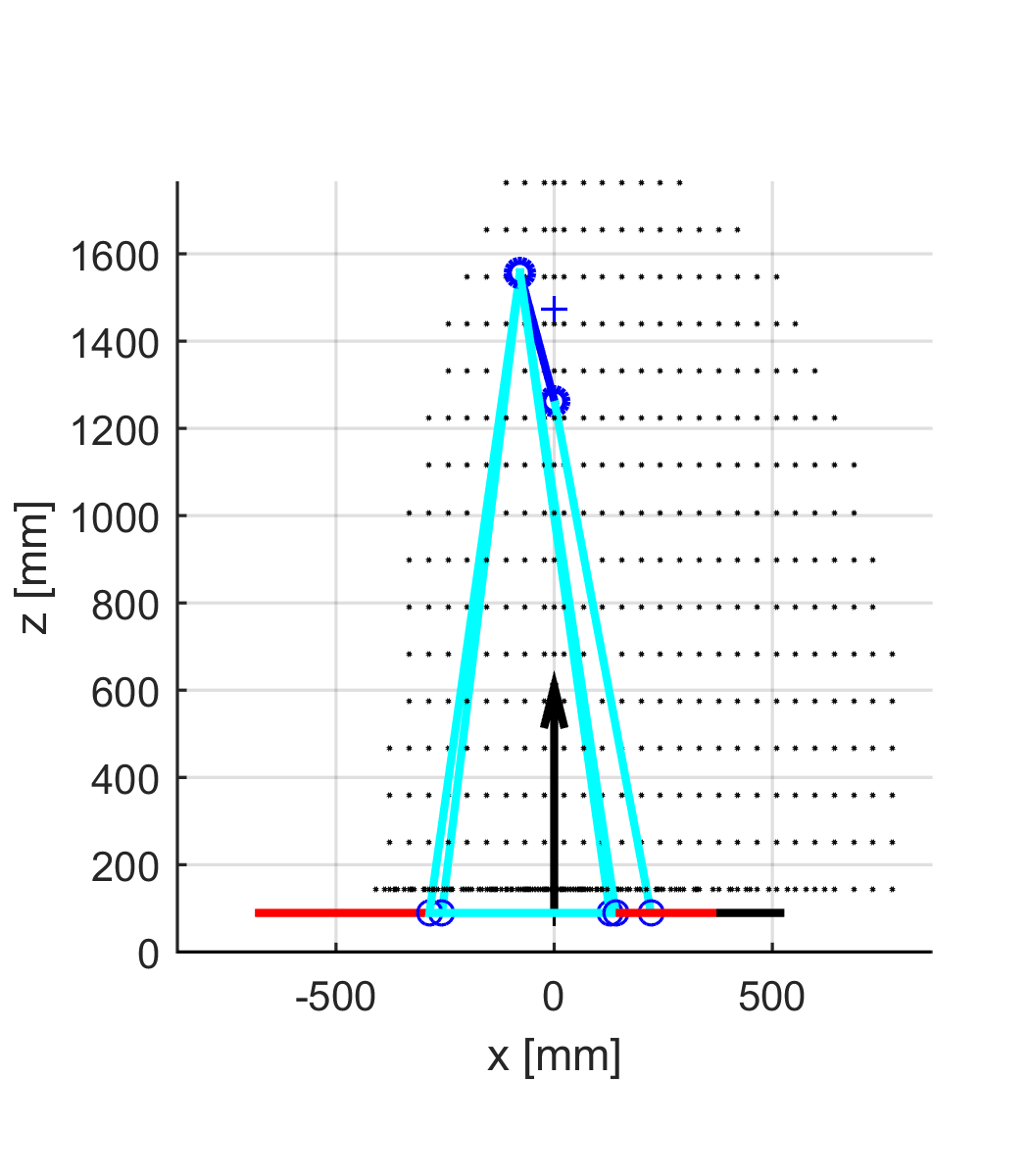
Based on the Kinematic Constraint Equations obtained previously, various kinematic properties can be evaluated through numerical analysis. The reachable space of a robot endpoint, or Workspace, is a fundamental kinematic property of robotic mechanisms. The envelope of the workspace is obtained numerically through the following procedure. First, a set of test points is generated in cylindrical coordinates $\left(r,\phi,z\right)$. For our analysis, the radius $r$ ranges from $0:L/2$, the angle $\phi$ ranges from $0:2\pi$, and the height $z$ ranges from $0:L$. These points were all converted to Cartesian coordinates relative to the robot origin, and the inverse kinematics are calculated for each. From the top plate pose, the three apices are computed with (3). The two Kinematic Constraint equations are then solved for actuator displacements $\left(s_{Ai},s_{Bi}\right)$. A test point is considered invalid if any of the actuator displacements is negative or complex as well as out of the linear actuator stroke. Such a point is not reachable and is not added to the list of valid points. The workspace envelope can be determined by repeating this examination for all the test points. Fig. 8-a, b, and c illustrate the workspace computed by examining the solutions to the Kinematic Constraint equations for the horizontal top plate configuration where $\Theta_{\epsilon}=0$. Fig. 8-d shows a side view of the workspace when the top plate is tilted about the Y axis, $\theta_{\epsilon}=75^{\circ}$.

Analysis of differential motion based on the Jacobian matrix relating the top plate velocity to the actuator velocities provides useful insights. The Jacobian can be computed for each top plate pose by differentiating the two Kinematic Constraint Equations in a way similar to the singularity analysis. Details can be found in [12]. Examining all the singular values of the Jacobian reveals the ability of TSE to move in 6-dimensional space. Similar analysis has been reported for different types of parallel manipulators [14]. Of particular interest for the current work is the Jacobian singular value in the vertical direction, $\sigma_{z}$, which can be considered the Spatial Gear Ratio between actuator motion and upward motion of the top plate. The highly extendable vertical motion is a salient feature of TSE. Numerical analysis reveals that the vertical singular value $\sigma_{z}$ varies widely depending on the height, while the singular values in the $XY$ horizontal directions are sufficiently large at diverse heights within a non-singular workspace. It is important to examine each TSE design in terms of these kinematic properties.

In order to perform generic analysis of the kinematic properties of the TSE, the Kinematic Constraint Equations must be distilled to the most essential design parameters. We non-dimensionalize equations (10) and (13) by scaling them by the total scissor length parameter $L$.

This leads to two new Kinematic Constraint Equations and four design parameters that define the entire design space for this class of machine:

• •

  $k_{1}$: $(\ell_{0}/L)$, the ratio of the lowest scissor link length and the total scissor length $L$. See Fig. 2.

• •

  $k_{2}$: $\eta$, the angle of the actuator from the horizontal axis of its respective coordinate frame. See Figs. 4 and 3.

• •

  $k_{3}$: $(r_{actuator}/L)$, the ratio of the actuator coordinate radial distance from center and $L$. See Figs. 4 and 6.

• •

  $k_{4}$: $(r_{top}/L)$, the ratio of the top platform distance to the ball joint and the total scissor length $L$. See Fig. 6.

The scissor top points $x_{C}$, $y_{C}$, and $z_{C}$ as well as the linear slide positions $S_{A}$ and $S_{B}$ are also normalized over the total scissor length $L$, which we define as $\hat{x_{C}}$, $\hat{y_{C}}$, $\hat{z_{C}}$, $\hat{S_{A}}$, and $\hat{S_{B}}$.

By rearranging and replacing variables in equations (10) and (13), the Non-Dimensionalized Kinematic Constraint Equations emerge. For the Delta configuration of linear actuators, they are given by

and

In order to judge one design of TSE against another, we use two performance metrics: the Height Amplification Factor $(HAF)$, and the Workspace Volume Percentage $(\%_{ws})$.

The Workspace Volume Percentage $(\%_{ws})$ is the percentage of the number of reachable test points examined within the cylindrical volume described previously.

The Height Amplification Factor ($HAF$) is given by

where $k_{i,0}$ is a constant design parameter selection to which all others are compared ($k_{1,0}=1$, $k_{2,0}=0^{\circ}$, etc). Note that by dividing the $z$-dependent singular value by another z-dependent singular value, the $HAF$ becomes constant throughout the $z$-range, and is no longer dependent on the configuration variable $z$. The $HAF$ may then be plotted directly against the design parameter $k_{i}$ for comparison.

In the previous subsection the Non-dimensionalized Kinematic Constraint Equations (19) and (20) were derived in order to facilitate the analysis of the kinematic properties of the TSE. In this section, we analyze how changing the kinematic design parameters $k_{1}$, $k_{2}$, $k_{3}$, and $k_{4}$ affect the configuration-dependent Translational Spatial Gear Ratios of the TSE and the Workspace Volume Percentage as defined previously.

For these analyses, the design parameters chosen match those of the implemented prototype and a single design parameter was changed each time to determine how deviating from this design affects the HAF and Workspace Volume Percentage.

References

- [1] D. Stewart, “A Platform with Six Degrees of Freedom,” Proceedings of the Institution of Mechanical Engineers, vol. 180, no. Pt 1, No 15, 1965.
- [2] E. Gough, “Contribution to discussion of papers on research in Automobile Stability, Control and Tyre performance,” in Proceedings of the Institution of Mechanical Engineers: Automobile Division, 1956, pp. 392–394.
- [3] V. Kumar, “Characterization of Workspaces of Parallel Manipulators,” ASME Journal of Mechanical Design, vol. 114, no. SEPTEMBER 1992, pp. 368–375, 1992.
- [4] Z. Huang, Q. Li, and H. Ding, Theory of Parallel Mechanisms. Springer Netherlands, 2013.
- [5] J. Angeles, Fundamentals of Robotic Mechanical Systems: Theory, Methods, and Algorithms, 4th ed. Springer International Publishing, 2014.
- [6] D. Jakobovic and L. Jelenkovik, “The Forward and Inverse Kinematics Problems for Stewart Parallel Mechanisms,” in 8th International Scientific Conference on Production Engineering: Computer Integrated Manufacturing and High Speed Machining (CIM2002),, 2002, pp. II–001 – II–012.
- [7] J.-P. Merlet, C. M. Gosselin, and N. Mouly, Workspaces of Planar Parallel Manipulators. Vienna: Springer Vienna, 1997, pp. 37–44. [Online]. Available: http://dx.doi.org/10.1007/978-3-7091-2666-0_5
- [8] Z. Wang, S. Ji, Y. Li, and Y. Wan, “Robotics and Computer-Integrated Manufacturing A unified algorithm to determine the reachable and dexterous workspace of parallel manipulators,” Robotics and Computer Integrated Manufacturing, vol. 26, no. 5, pp. 454–460, 2010. [Online]. Available: http://dx.doi.org/10.1016/j.rcim.2010.02.001
- [9] A. L. Orekhov, C. E. Bryson, J. Till, S. Chung, and D. C. R. Member, “A Surgical Parallel Continuum Manipulator with a Cable-Driven Grasper,” in 2015 37th Annual International Conference of the IEEE Engineering in Medicine and Biology Society (EMBC), Milan, 2015, pp. 5264–5267.
- [10] D. Chablat and L. Rolland, “Design of mechanisms with scissor linear joints for swept volume reduction Design of mechanisms with scissor linear joints for swept volume reduction,” in 4th Joint International Conference on Multibody System Dynamics (IMSD), Montréal, Québec, Canada, 2016.
- [11] J. Yang, X. Wang, and X. F. Chen, “Dynamic Identification of a 3-PRS Parallel Robot with Scissor-Type Prismatic Joint: A Cloud-Based Approach,” in Mechanisms and Machine Science: Advances in Reconfigurable Mechanisms and Robots II. Springer, 2015, pp. 339–350.
- [12] D. J. Gonzalez and H. H. Asada, “Triple Scissor Extender : A 6-DOF Lifting and Positioning Robot,” in Proceedings of the IEEE International Conference on Robotics and Automation, 2016.
- [13] C. Gosselin and J. Angeles, “Singularity analysis of closed-loop kinematic chains,” IEEE Transactions on Robotics and Automation, vol. 6, no. 3, pp. 281–290, jun 1990.
- [14] J. P. Merlet, “Jacobian, Manipulability, Condition Number, and Accuracy of Parallel Robots,” Springer Tracts in Advanced Robotics: Robotics Research: Results of the 12th International Symposium ISRR, vol. 28, pp. 175–184, 2007.