Deriving the slip front propagation velocity with the slip- and slip-velocity-dependent friction laws via the use of the linear marginal stability hypothesis
Abstract
We analytically and numerically investigate the determining factors of the slip front propagation (SFP) velocity. The slip front has two forms characterized by intruding or extruding front. We assume a 1D viscoelastic medium on a rigid and fixed substrate, and we employ the friction law depending on the slip and slip velocity. Despite this dependency potentially being nonlinear, we use the linear marginal stability hypothesis, which linearizes the governing equation for the slip, to investigate the intruding and extruding front velocities. The analytically obtained velocities are found to be consistent with the numerical computation where we assume the friction law nonlinearly depends on both the slip and slip velocity. This implies that the linearized friction law is sufficient to capture the dominant features of SFP behavior.
I Introduction
The slip front propagation (SFP) is an important phenomenon in several scientific and technological fields, including frictional sliding on the interface between two media and crack tip propagation in a medium. From a theoretical viewpoint, researchers have investigated SFP using both discrete Lan93 ; Amu1 ; Amu2 ; Tro and continuum Rad ; Suz19 models. Furthermore, laboratory experiments have also been performed to investigate SFP Ben . Geophysical studies have also contributed to the understanding of the SFP behavior because fault tip propagation can be modeled as SFP. The SFP velocity has attracted considerable research interest. For example, ordinary and slow earthquakes are widely known to exist Oba ; Kat , and they have different SFP velocities; the SFP velocities for the former category of the earthquake are much higher than those of the latter. The origin of this difference remains an important open research question.
The friction law plays an important role in the understanding of SFP. For example, a friction stress depends on the state variable in the rate-and-state dependent friction model Amu2 ; Bar13 ; Rad . Bar-Sinai et al. Bar13 investigated the SFP velocity using a semi-infinite continuum model and the rate-and-state friction law. Furthermore, we note that the friction stress can also depend on quantities such as the slip and slip velocity. For example, Myers and Langer Mye employed a spring-block model with a slip-velocity-weakening law to study the SFP velocity. The rate-and-state dependent friction law with the shear stiffness of the contacts can be interpreted as the slip-strengthening behavior Bar12 . Moreover, the friction law depending on the slip and slip velocity is realized for elasto- and visco-dampers Hib03 ; Hib05 . The slip- and slip-velocity- dependences of friction stress is important in geophysical studies Ika ; Ito .
Additionally, the viscosity of the medium is important in understanding the SFP behavior Ots ; Mye ; Suz19 . Our previous study Suz19 analyzed an infinitely long viscoelastic block on a rigid substrate and achieved the systematic understanding of the SFP velocity in terms of the viscoelasticity and the friction law depending on the slip velocity in a quadratic manner. Despite these studies, a thorough investigation of the SFP velocity with viscoelastic medium and a friction law that depends on the slip and slip velocity has not yet been undertaken.
Spontaneous SFP velocity has been widely understood by regarding the phenomenon of SFP as the evolution of a solution of the governing equation from a stable state into an unstable state and employing the linear marginal stability hypothesis (LMSH) Lan91 ; Mye ; Suz19 . The LMSH has been widely used to investigate the dynamics of fronts or domain walls that propagate spontaneously into an unstable state in a model with a nonlinear governing equation Saa1 ; Saa2 . This approach has been used to obtain the solidification front speed Dee , the chemical reaction front speed Saa1 ; Saa2 , and the slip front velocity between blocks and substrates Lan91 ; Suz19 ; Mye . This hypothesis asserts that even if the governing equations are nonlinear, a linearized model yields sufficiently accurate front behavior, including the correct front propagating velocity. This hypothesis has been applied to the slip front behavior via the linearization of the friction law; the friction laws adopted in such studies have been limited, e.g., the slip-velocity-weakening Lan91 ; the systematic treatment of various types of friction law has not been performed.
This paper is organized as follows. A brief introduction to the LMSH is provided in Sec. II.1, and the model setup is defined in Sec. II.2. Analytical treatment of the problem is presented in Sec. III; in this section several SFP velocities are obtained based on the LMSH, and a discussion of their physical implications are presented. The numerical treatment and implications for slip behavior are discussed in Sec. IV, and the treatment of the LMSH is justified there. A summary and discussion are presented in Sec. V.
II MODEL WITH VELOCITY-DEPENDENT LOCAL FRICTION LAW
II.1 Linear Marginal Stability Hypothesis (LMSH)
The LMSH has been widely used to investigate the dynamics of fronts or domain walls that propagate spontaneously into an unstable state where the phenomena are described by nonlinear governing equations Saa1 ; Saa2 . This approach has been used to obtain the solidification front speed Dee , the chemical reaction front speed Saa1 ; Saa2 , and the SFP velocity Mye ; Suz19 ; Lan91 . We briefly summarize this approach here. The LMSH requires linearizing the governing equation, the plane wave approximation of the solution near the propagating front, and the two conditions associated with the stability of growth of the disturbance and that of propagation. This hypothesis states that the characteristic frequency, the wave number, and the propagating velocity of a front can be derived even after these approximations.
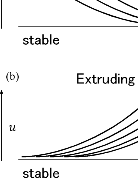
To understand the details of LMSH further, we define as a variable characterizing the state of the system (in the case of motion of a continuum, this variable could be slip); we consider the dynamics of the spontaneous propagation of . Here we assume an infinite and 1D system. We consider two cases: (1) is unstable and the stable region with intrudes into this unstable region, and (2), is stable and this region intrudes into the unstable region with . The front in the former case is referred to as an “intruding front,” whereas that in the latter case is called an “extruding front” (Fig. 1). Notably, if the governing equation of is a wave equation, the cases are symmetric and the propagation velocity is equal in magnitude. However, if the governing equation includes additional terms, such as a diffusion term, the symmetry vanishes, and different propagation velocities are expected for the two fronts.
The front is mathematically defined to be located where terms of dominate and terms of become negligible in the governing equations. For the solution of , we assume the plane wave solution, , whose frequency and wave number are complex in the region close to the front. The upper (lower) sign corresponds to the intruding (extruding) front propagation. To understand this propagation, we rewrite this plane wave solution of as
| (1) |
where and are the real and imaginary parts of , respectively, and and are the real and imaginary parts of , respectively. Notably, the absolute value of Eq. (1) can determine the front, i.e., is used to define the front. The value of describes the oscillation within the envelope , and is not used to determine the position of the front. Equation (1) and Fig. 1 clearly indicate that the upper (lower) sign corresponds to the intruding (extruding) front. In the above expression, and are four unknown parameters, and the LMSH determines them via four independent equations: the real and imaginary parts of the dispersion relation and the expressions for growth and propagating stabilities. With these values, the primary goal of this study is obtaining an analytical form for the intruding and extruding front velocity.
The growth stability condition mentioned above is given by
| (2) |
whereas, the propagating stability is given by the relationship:
| (3) |
where is a positive constant. The remaining equations are given by
| (4) |
and
| (5) |
which are obtained from the Cauchy-Riemann relationship.
Equation (2) represents the condition that the disturbance will not grow with increasing time. Equation (3) indicates that the phase velocity is equal to the group velocity . Given that the disturbance propagates with the group velocity, this condition dictates that the disturbance and the front propagate with the same velocity. It is important to note that for stability, the relationship is sufficient because the disturbance is overtaken by the front with . Nonetheless, Ref. Saa1 mathematically showed that Eq. (3) is satisfied for spontaneous front propagation. For more details regarding these conditions see Ref. Suz19 .
II.2 Model setup
In this work we consider a semi-infinite viscoelastic medium that is assumed to be on the rigid and fixed substrate. We apply a loading stress on the left end of the medium in the direction tangential to the substrate surface, i.e., an end-loading stress. We employ the nondimensionalization of the variables based on Ref. Suz19 . The end-loading stress is denoted , and this constant stress is applied along the axis for a time . We also consider additional loading conditions. Among the loading conditions, we evaluate in this work the continuum limit of the Burridge-Knopoff model, which includes a driving stress from the upper block connected to the upper plate Mye . We refer to this loading stress as “upper-loading stress.” The upper-loading stress is denoted , and this constant stress is applied along the axis for the time . We assume that is less than the macroscopic maximum static friction stress, which is assumed to be the same for all the blocks considered. We treat the two models (with the different loading conditions) in the single framework: the model subject to the end-loading stress is referred to as the EL model, whereas the model with end- and upper-loading stresses is called the EUL model. In these models, the system is considered to be 1D along the axis, and the slip distance, , at position and time is zero throughout the whole system for .
We can consider the nondimensionalized governing equation:
| (6) |
where is a slip-dependent function describing the loading condition, and describe the local friction stresses that depend on and , respectively, and the dot and prime represent differentiation with respect to and , respectively. The loading conditions can be treated systematically via the function . We can select for the EL model Suz19 , and for the EUL model Mye . The terms , , and have a physical interpretation; they represent the inertia, elastic, and viscous terms, respectively. This viscous term is employed in several previous studies Mye ; Suz19 .
Several forms of and have been considered in the analysis of SFP (e.g., Lan91 ; Mye ; Suz19 ), and the SFP velocity has been analytically investigated previously Suz19 . The purpose of the present paper is to derive a more universal expression for SFP velocity, which is independent of the details of friction laws; such an analysis enables us to understand the SFP behavior in the single framework.
III Analytical treatment
We now linearize the terms from Eq. (6). We take
| (7) |
where and are constants. To undertake the linearization (7), we assume that the system is in a critical state before the end-loading in the EUL model, which leads to
| (8) |
Analyses without the critical state assumption have been performed in previous studies Mye ; Bar12 . However, those treatments only provide approximations for the SFP velocities. With the assumption of the critical state, an analytical treatment is possible here.
We note that if the slip direction reverses ( turns to be negative) with increasing time, Eq. (7) cannot be applied. The reason for this is twofold: firstly, the friction stress, , changes its sign if slip reversal occurs, and thus, the linearization of Eq. (7) cannot be employed. Secondly, if the slip reversal occurs, the absolute value of the stress acting on the slip-reversal point will exceed the maximum static friction stress. This slip criterion is not considered in the linearization of Eq. (7). We do not consider the slip reversal in the following analytical treatment, as is done in seismology Suz06 .
Using the linearization of Eq. (7), we rewrite the governing equation [Eq. (6)],
| (9) |
We note positive and negative values for and are permitted.
We assume the plane wave solution for Eq. (9), i.e., . The upper (lower) sign describes the intruding (extruding) front propagation, as noted in Sec. II.1. Based on this assumption and using Eq. (9), the dispersion relation is found to be
| (10) |
Considering the real and imaginary parts of the dispersion relation in Eq. (10), we obtain,
| (11) |
| (12) |
respectively. We first note that the solutions and exist. In the case of and being positive and , the solution set exists. The solutions and describe an oscillating solution. The slip reversal occurs with these solutions; such solutions cannot be treated in a framework based on Eq. (9). Thus, this solution set is excluded from the following discussion. We therefore assume in the analytical treatment. With such an assumption, considering Eq. (11), we have
| (13) |
Combining this equation, the expression for growth stability [Eq. (2)] and condition for propagation stability [Eq. (3)], we obtain a cubic equation for ,
| (14) |
and a relationship between and :
| (15) |
We begin by categorizing the solutions of Eq. (14) in terms of the numbers of positive and negative real solutions. Combining the results with Eq. (15), we are able to investigate the numbers of SFP velocities that the above equations yield.
We start by defining as being equal to the left-hand side of Eq. (14) with the upper sign; such a definition permits us to study the intruding front velocity. It is noted that the discussion performed in this section is also directly applicable to the extruding front propagation. To confirm this statement, we define as the left-hand side of Eq. (14) with the lower sign. We then have the relationship
| (16) | |||||
Thus, we see that the number of the real solutions for is exactly the same as the number of real solutions for , and the positive (negative) solutions for the former correspond to the negative (positive) solutions for the latter. We therefore investigate only the numbers of real solutions for in this work.
To categorize the numbers of the real solutions for in terms of and , we require an expression for , , and , where
| (17) |
and is defined as the solution of
| (18) |
which leads to the solution
| (19) |
(double signs in the same order). We observe that if is positive is real. Additionally, we can obtain
| (20) |
and
| (21) |
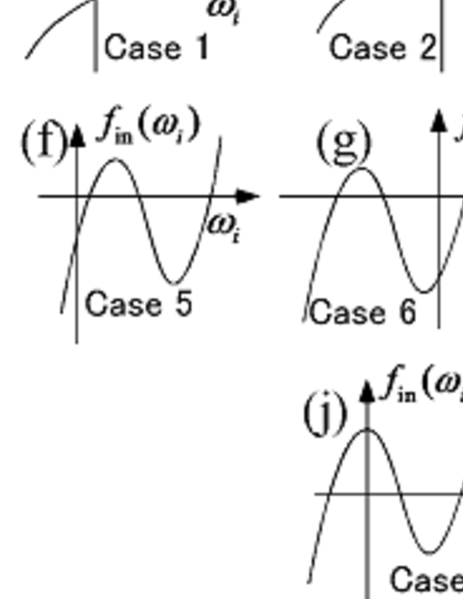
We define , , and as the solutions for ; is defined to always take real values, as described in Appendix A. We number the various cases based on the diagram shown in Fig. 2(a). In cases 1, 2, 3, 4, 7, and 8, only is real, and is positive in cases 1, 3, and 4, whereas it is negative in cases 2, 7, and 8. Though the numbers of the positive (negative) solutions are the same for the cases 1, 3, and 4 (2, 7, and 8), we differentiate the cases because the numbers of the real positive solutions for , which is one or zero, may be different in each case. The solutions , , and are real in cases 5, 6, 9, and 10. All the solutions are positive in case 5, two are positive and one is negative in case 9, two are negative and one is positive in case 6, and all the solutions are negative in case 10.
We now obtain the analytical forms of the boundaries dividing cases 1–10 in phase space. These equations are obtained based on the diagram Fig. 2(a) as follows:
| (22) |
| (23) |
| (24) |
| (25) |
| (26) |
| (27) |
First, using Eqs. (17) and (22), we obtain a boundary referred to as boundary A, which reduces to the parabolic form
| (28) |
From Fig. 2, boundary A represents a boundary between a region in which solutions are characterized as cases 1–2 and a region containing solutions that fall into cases 3–10 in the space. Next, from Eqs. (20) and (23), we can conclude that represents a boundary, which we will call boundary B. Boundary B divides regions of solutions that are represented as case 1 from case 2, and the solutions in cases 3–6 from cases 7–10. Further, we consider the cubic equation for from Eqs. (21), (24), and (25):
| (29) | |||||
We can factorize this equation to obtain,
| (30) |
which we can evaluate to find that
| (31) |
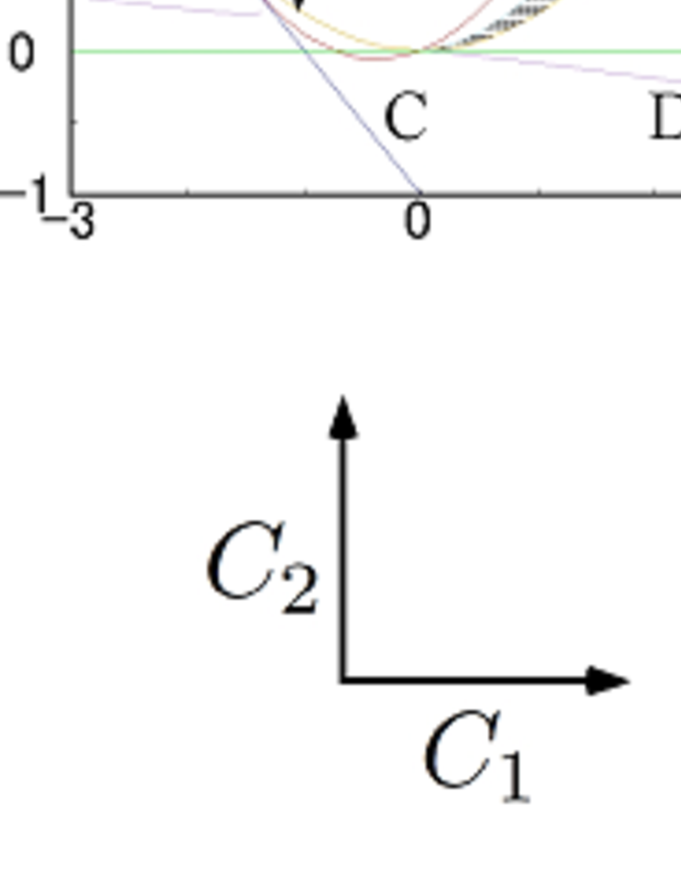
are boundaries. The former will be referred to as boundary C, and the latter will be referred to as boundary , respectively (double signs in the same order). Boundary C is a boundary for regions where solutions are of case 3, case 4, and cases 5–6, and divides the regions in which solutions in case 7, case 8, and cases 9–10 exist. Additionally, we can confirm analytically that the boundaries A, C, and all pass through the point , and that the boundary C is tangential to the boundaries A and at this point.
Using the boundaries , we obtain the phase space that categorizes the behavior of the solutions for (see Fig. 3). Figure 3 shows that cases 6, 7, 8, and 10 are further divided into two disconnected regions. Actualy, from Eqs. (19), (26), and (27), we can obtain the relationship for [Eq. (27)] and for [Eq. (26)]. This forms a boundary between regions in which solutions for fall into cases 5 and 6, and cases 9 and 10. However, we can see that the case 5 does not appear in the phase space (see Fig. 3), and case 9 is not adjacent to case 10. Therefore, this straight line does not appear as a boundary in Fig. 3.

The solutions for have been categorized in the space. We now categorize the solutions for . Notably, the solution for is obtained from Eq. (15); thus we see that the solution does not exist when the right-hand side of Eq. (15) is negative, even if real and positive solutions for exist. Therefore, we see that the curve is another boundary in the space. We refer to this boundary as boundary E, and the analytical form of the boundary E is obtained here. If we substitute to Eq. (13) with the upper sign, we obtain
| (32) |
where the sign of the second term on the right-hand side is arbitrary. Substituting in Eq. (15) with the upper sign yields
| (33) |
From the two previous expressions, an equation describing boundary E can be obtained:
| (34) |
It can also be confirmed that boundary C is a tangent to boundary E at the point . The phase space is shown in Fig. 4. This figure shows 17 subdivided regions of the cases, and they are named as shown in the figure (see Table 1 for details).
We show the values of , , , and () in Fig. 5, where , , and are defined in Appendix A. Note that and do not exist. The values of , , and are zero on boundary E. Note that since Eq. (34) is a necessary and not a sufficient condition for or , non-zero values ( and ) are allowed on bounary E.
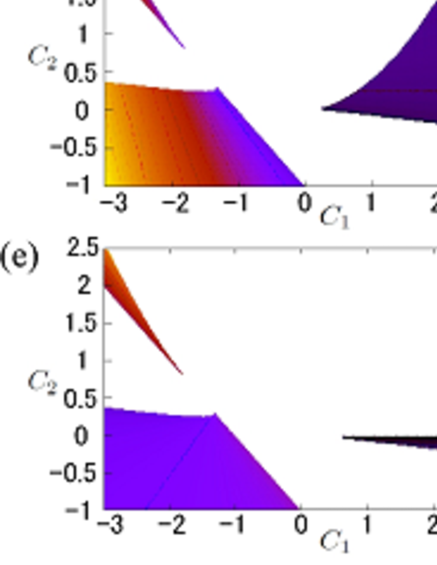
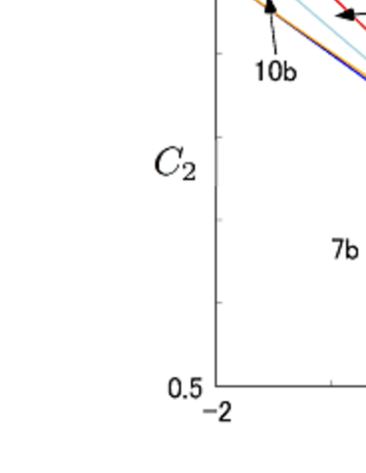
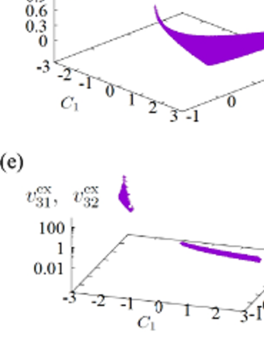
Using the values of , , , and corresponding to solutions of , we also investigate the intruding front velocity, , and the extruding front velocity, . We define the th intruding and extruding front velocity as and , respectively, as in Appendix A, and the velocities , , , and exist. The regions where , , , , and exist are shown in Fig. 6(a–e), respectively, in space. We note that the region where exists is separated into two disconnected regions. We refer to which corresponds to values of negative as , and that which corresponds to positive values of as . We have three velocities in cases 6a and 9b (, , for case 6a and , , for case 9b). There exist two velocities in cases 9a and 10d ( and for 9a and and for 10d). For cases 1, 4, and 6b, we obtain the single velocity , whereas in cases 2a, 7a, 8b, and 10b, only a single velocity is found to exist. Finally, we note that no solutions for or exist in cases 2b, 7b, 8a, 8c, 10a, and 10c.
The values of the front velocities , , , , , and are shown in Fig. 7. It is found that , , and diverge close to boundary E. This divergence is because the values of , , and are equal to zero, while , , and take non-zero values, on the boundary. We can therefore conclude that these velocities describe optical modes and represent unphysical propagations. In addition, we confirmed that the velocities and take the values and , respectively, on the axis for . These values are consistent with those found in Ref. Suz19 because the slip-dependence of the friction stress was negelected in that work, i.e., . The value of is not consistent with . We therefore conclude that and represent the physical SFP velocities for the intruding and extruding fronts, respectively. We can also suggest that and are the extension of the intruding and extrding front velocities obtained in Ref. Suz19 to the model with the friction law depending on the slip and slip velocity.
IV NUMERICAL TREATMENT: IMPLICATIONS FOR SLIP BEHAVIOR
In this section we show the spatiotemporal evolutions of the slip velocity found via numerical computations using the values shown in Table 1. We confirm that the values of and obtained using the LMSH are accurate.
| Cases | Velocity | ||
| 1 | |||
| 2a | 1 | 2 | |
| 2b | 0.2 | ||
| 4 | 1 | ||
| 6a | 1 | ||
| 6b | |||
| 7a | 1 | 0.5 | |
| 7b | 0.5 | ||
| 8a | 0.05 | ||
| 8b | 2.75 | ||
| 8c | 0.71 | ||
| 9a | 1 | 0.1 | |
| 9b | 1 | 0.3 | |
| 10a | 0.1 | ||
| 10b | 2.5 | ||
| 10c | 0.755 | ||
| 10d | 2.125 |
IV.1 Intruding front propagation
In this section we numerically consider the intruding front velocities. We consider because does not exist and describes an optical mode, which represents an unphysical propagation. As such, we treat the cases 1, 4, 6a, 6b, 9a, and 9b (see Table 1). We consider the EUL model, i.e., . In the following, we assume .
For the numerical computations a friction law must be determined. There are few restrictions on the choice of friction laws provided they are reduced to the form of Eq. (7) via linearization. Here, we adopt following expression for :
| (35) | |||||
In this model, the system is in a critical state at the onset of end-loading, i.e., , as assumed in Sec. III. Additionally, it is possible to show that the right-hand side of Eq. (35) is always positive for any positive values of and , which is a required condition for the friction laws. We define the slip front as the region where and are sufficiently small that only their linear terms exist in Eq. (35), and with this assumption, we can derive the relation
| (36) |
from Eq. (35), which is seen to be equivalent to Eq. (7). Though the friction law (35) looks artificial, we emphasize that this expression is an example which permits numerical calculations and allows us to confirm the validity of the analytical treatment presented in this work.
To permit numerical calculations, the system must be finite, whereas an infinite system was assumed in the analytical treatment. We assume that the end-loading point is located at the position for the finite system employed for the numerical calculations, and we use the value of as the end-loading stress, instead of in the analytical work. In the numerical work, the Runge-Kutta method with fourth-order accuracy is used.
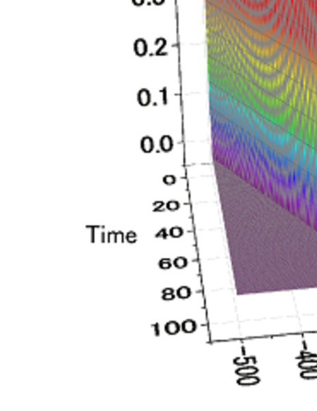
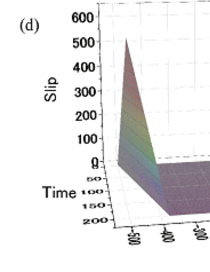
We can then numerically obtain the spatiotemporal evolutions of the slip velocities, which are shown in Fig. 8. Figure 8 shows that all the cases considered here generate intruding front velocities which are in agreement with those obtained analytically. This indicates that the LMSH is effective and that the normalized form of the governing equation accurately determines the SFP behavior. We note that the slip velocity profile is pulse-like in Fig. 8, which is clearly shown in Fig. 9. This result indicates that the slip velocity is always positive, and that the slip reversal does not occur when the stated friction law is considered [Eq. (35)].
The supersonic front propagation is observed in Fig. 8(b), (c), (e) and (f); the shear wave velocity is unity in the present framework. These cases correspond to the slip- and/or slip-velocity-weakening behaviors with the critical condition just before the slip. Though the treatment in this study is not the same as that of the crack-tip propagation, the front propagation obtained here may be consistent with the supersonic crack-tip propagations addressed in previous studies Bue03 ; Bue06 ; Mar ; Gia .
IV.2 Extruding front propagation
Here we consider the extruding front velocities. We consider only because and correspond to the optical modes, and the value of is not consistent with that of previous study. To simulate the extruding front, we consider the EL model Suz19 .
In this numerical work, we assume the following friction laws,
| (37) |
and
| (38) |
where , and are positive constants. The friction laws given in Eqs. (37) and (38) assume a quadratic dependence of the friction stress on the slip velocity and slip, respectively. The quadratic dependence of the slip velocity was assumed in Ref. Suz19 , and this dependence is now extended to the slip dependence. In the following discussion it is shown that the friction laws in Eqs. (37) and (38) generate the extruding front.
First, we demonstrate that the friction laws (37) and (38) do not generate the intruding front propagation. These friction laws state that the system corresponds to and when and . As shown in Fig. 6(a), does not exist in the region in which and . Therefore, under these conditions we do not have an intruding front propagation.
Here we demonstrate how the extruding front velocity is determined with the friction laws given in Eqs. (37) and (38). We first introduce the variable,
| (39) |
where is a positive constant. From the definition in Eq. (39), we obtain,
| (40) |
where is an arbitrary function of . We consider the region near the slip front propagating with a constant velocity. Therefore, if we assume that is equal to the extruding front velocity, we can see that is a constant, which results in
| (41) |
where is a positive constant. We assume that and are sufficiently small to mean that the terms of order and and higher can be neglected. Using Eqs. (6), (37), (38), (39), and (41), considering only the linear terms of and , we obtain the governing equation:
From these expressions, we conclude that the values and in Eq. (9) are given by:
| (43) |
and
| (44) |
Here, we demonstrate a method determining the values of and . First, we write as a function of and , i.e., . This function is illustrated in Fig. 7(i). We then define the values of and . Since the quantities and are the gradients of and , respectively, at and , we obtain
| (45) |
and
| (46) |
around and . Therefore, the equation
| (47) |
yields a relation between and . Since depends on , the above expression represents a self-consistent equation. However, we cannot determine the two unknown quantities, and , uniquely from this single equation. We obtain a second expression relating the two parameters via consideration of . We assume that the single relation
| (48) |
exists, whereas obtaining the analytic form of is impossible. However, we can expect that a larger value of induces a larger value of . Equations (47) and (48) determine the extruding front velocity for a given . Finally, if these equations do not have the solution, the steady SFP does not exist.
Here, we show how the analytical treatment and numerical calculations are consistent with Eqs. (37) and (38). First, we set the values of , and . We then numerically compute the spatiotemporal evolutions of the slip, and the slip front is roughly determined from the slip-velocity profile. We also roughly evaluate the slip and slip velocity at the front; these values correspond to and , respectively. With , obtained, using Eqs. (37) and (38) we obtain the values of and ; thus we can obtain because it is a function of and . We then estimate the SFP velocity at the determined front from the numerical computations; the velocity obtained using this estimate is denoted . We finally confirm that is approximately equal to .
It remains, however, to confirm another condition: as observed, in the analytical treatment, the inequalities and must be satisfied at the slip front. These conditions are satisfied when and , in the numerical treatment. It should be confirmed that these relations are satisfied in the numerical calculations.
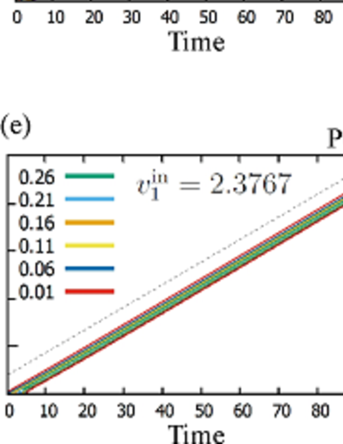
We consider an example with , and , and we apply the procedure described above (Fig. 10). In this case, as shown in Fig. 10(b), the gradient of the slip velocity profile along the axis is so large that it is not possible to determine the precise values of and . Therefore, we can only use an estimate for their values based on the profiles of the slip and slip velocity; in this case, we take and [see Fig. 10(b-e)]. The SFP velocity is relatively insensitive to variations around the values of and adopted here. These and values together with Eqs. (37) and (38) give the values and , which lead to . The SFP velocity obtained from the gradient of the dotted line in Fig. 10(a) is estimated to be . This almost coincides with the value of obtained above. Additionally, the conditions and are satisfied in this calculation. Thus, we have found good agreement between the analytic and numerical approaches in the obtained values of the extruding front velocity. Finally, we note the slip profile shown in Fig. 10(b) leads to the conclusion that the slip reversal does not occur in this case.
V DISCUSSION AND CONCLUSIONS
In this work we have considered an infinite 1D viscoelastic block on a substrate subject to end-loading stress and the end- and upper-loading stresses together with a friction law that depends on the slip and slip velocity. The two intruding front velocities and three extruding front velocities were analytically obtained based on the LMSH, which requires only the linearized governing equation. Of these five velocities, three represent the optical modes, and the unique intruding and extruding front velocities were found to exist for physically meaningful SFPs. Via numerical calculations, the intruding front velocity was obtained for the EUL model, and the extruding front velocity was realized for the EL model; these results indicated that the detail of the dependence of the friction stress on the slip and the slip velocity does not affect the front velocity, and that the linearized governing equation is sufficient to obtain accurate results.
Our framework is found to be quantitatively consistent with the results of previous studies. For example, the dependences of and on for are consistent with those of and in Ref. Suz19 , respectively, as mentioned in Sec. III. Additionally, the form of for is consistent with that obtained in Myers and Langer Mye . Though they obtained only an approximate solution, the exact analytical solution has been obtained here. Furthermore, note that their model corresponds to the case , and they changed parameters and , where is the viscosity, and corresponds to . Therefore, both their and our models have two parameters. However, our model is superior because we can treat both positive and negative in a single framework. Moreover, we were successful in explaining the variation in SFP velocities using only friction laws with constant viscosity.
We also have shown the regions in which the SFP velocities exist in the phase space; we also have presented the analytical forms of the boundaries of these regions in the phase space. This phase space may be useful to predict, e.g., whether ordinary or slow earthquakes are likely in natural faults, if the friction law is determined.
Since LMSH linearizes the governing equations, it cannot give an estimation of the macroscopic slip profile. Note that the pulse-like slip was observed in Fig. 9, and the step-function-like slip emerged in Fig. 10. These are consistent with previous laboratory experiments Nie or seismological observations Das ; Aag . Nonetheless, predicting these slip behaviors is difficult with the present framework.
Finally, the critical state was assumed for the EUL model. Based on this assumption, we can proceed with the analytical treatment. In reality, the SFP in a non-critical state has been analyzed Mye ; Bar12 , and the SFP velocities have been obtained. They are, however, approximations. Though the current treatment cannot be directly applied to the non-critical case, we anticipate that it will be an important step in analytically treating SFP velocities with the non-critical state.
Appendix A Exact Solutions of
Here, we present details of the analytical treatment of . This is the cubic equation, and we can solve it analytically. We first define the variables and :
| (A1) |
and
| (A2) |
Using Eqs. (A1) and (A2), we define
| (A3) |
(double signs in the same order), which can take complex values. With these values and the cubic root of unity, , we obtain:
| (A4) |
| (A5) |
| (A6) |
If is real and negative, is defined as . Therefore, always gives a real-valued solution. With Eqs. (A4)(A6) and Eq. (15), we can define and (). We note that if , we can conclude that does not exist. We can use exactly the same method to solve and to define and .
Acknowledgements.
T. S. was supported by JSPS KAKENHI Grant Number JP20K03771, and JSPS KAKENHI Grant Number JP16H06478 in Scientific Research on Innovative Areas “Science of Slow Earthquakes.” This study was supported by the Ministry of Education, Culture, Sports, Science and Technology (MEXT) of Japan, under its The Second Earthquake and Volcano Hazards Observation and Research Program (Earthquake and Volcano Hazard Reduction Research). This study was supported by ERI JURP 2020-G-08, 2021-G-02 and 2022-G-02 in Earthquake Research Institute, the University of Tokyo.References
- (1) J. S. Langer, and H. Nakanishi, Phys. Rev. E, 48, 439-448 (1993).
- (2) D. S. Amundsen, J. Scheibert, K. Thøgersen, J. Trømborg, and A. Malthe-Sørenssen, Tribol. Lett., 45, doi:10.1007/s11249-011-9894-3 (2012).
- (3) D. S. Amundsen, J. K. Trømborg, K. Thøgersen, E. Katzav, A. Malthe-Sørenssen, and J. Scheibert, Phys. Rev. E, 92, doi:10.1103/PhysRevE.92.032406 (2015).
- (4) J,. K. Trømborg, H. A. Sveinsson, K. Thøgersen, J. Scheibert, and A. Malthe-Sørenssen, Phys. Rev. E., 92, doi:10.1103/PhysRevE.92.012408 (2015).
- (5) M. Radiguet, D. S. Kammer, P. Gillet, and J.-P. Molinari, Phys. Rev. Lett., 111, doi:10.1103/PhysRevLett.111.164302 (2013).
- (6) T. Suzuki, and H. Matsukawa, J. Phys. Soc. Jpn., 88, 114402 (2019).
- (7) O. Ben-David, G. Cohen, and J. Fineberg, Science, 330, 211-214 (2010).
- (8) K. Obara, Science, 296, 1679-1681 (2002).
- (9) A. Kato, K. Obara, T, Igarashi, H. Tsuruoka, S. Nakagawa, and N. Hirata, Science, 335, doi:10.1126/science.1215141 (2012).
- (10) Y. Bar-Sinai, R. Spatschek, E. A. Brener, and E. Bouchbinder, Phys. Rev. E, 88, doi:10.1103/PhysRevE.88.069905 (2013).
- (11) C. R. Myers, and J. S. Langer, Phys. Rev. E, 47, 3048-3056 (1993).
- (12) Y. Bar-Sinai, E. A. Brener, and E. Bouchbinder, Geophys. Res. Lett., 39, L03308, doi:10.1029/2011GL050554, 2012
- (13) H. Hibino, M. Takaki, and S. Katsuta, J. Struct. Constr. Eng., AIJ, 574, 45-52 (2003) (in Japanese with English abstract).
- (14) H. Hibino, M. Takaki, and S. Katsuta, J. Struct. Constr. Eng., AIJ, 593, 43-50 (2005) (in Japanese with English abstract).
- (15) M. J. Ikari, C. Marone, D. M. Saffer, and A. J. Kopf, Nat. Geosci., 6, 468-472, doi:10.1038/ngeo1818 (2013).
- (16) Ito, Y., and M. J. Ikari, Geophys. Res. Lett., 42, 9247-9254 (2015).
- (17) M. Otsuki, and H. Matsukawa, Sci. Rep. 3, doi:10.1038/srep01586 (2013).
- (18) J. S. Langer, and C. Tang, Phys. Rev. Lett., 67, 1043-1046 (1991).
- (19) W. van Saarloos, Phys. Rev. A., 37, 211-229 (1988).
- (20) W. van Saarloos, Phys. Rev. A, 39, 6367-6389 (1989).
- (21) G. Dee, and J. S. Langer, Phys. Rev. Lett., 50, 383-386 (1983).
- (22) T. Suzuki, and T. Yamashita, J. Geophys. Res., 111, B03307, (2006).
- (23) M. J. Buehler, F. F. Abraham, and H. Gao, Nature, 426, 141-146 (2003).
- (24) M. J. Buehler, and H. Gao, Nature, 439, 307-310 (2006).
- (25) M. Marder, J. Mech. Phys. Solids, 54, 491-532 (2006).
- (26) A. E. Giannakopoulos, and A. J. Rosakis, J. Appl. Mech., 87, 061004 (2020).
- (27) S. Nielsen, J. Taddeucci, and S. Vinciguerra, Geophys. J. Int., 180, 697-702 (2010).
- (28) S. Das, Pure Appl. Geophys., 160, 579-602 (2003).
- (29) B. T. Aagaard, and T. H. Heaton, Bull. Seism. Soc. Am., 94, 2064-2078 (2004).