Derivative based global sensitivity analysis and its entropic link
School of Physics, Engineering and Technology
University of York
Heslington, York, YO10 5DD, UK
[email protected]
Abstract
Variance-based Sobol’ sensitivity is one of the most well known measures in global sensitivity analysis (GSA). However, uncertainties with certain distributions, such as highly skewed distributions or those with a heavy tail, cannot be adequately characterised using the second central moment only. Entropy-based GSA can consider the entire probability density function, but its application has been limited because it is difficult to estimate. Here we present a novel derivative-based upper bound for conditional entropies, to efficiently rank uncertain variables and to work as a proxy for entropy-based total effect indices. To overcome the non-desirable issue of negativity for differential entropies as sensitivity indices, we discuss an exponentiation of the total effect entropy and its proxy. We found that the proposed new entropy proxy is equivalent to the proxy for variance-based GSA for linear functions with Gaussian inputs, but outperforms the latter for a river flood physics model with 8 inputs of different distributions. We expect the new entropy proxy to increase the variable screening power of derivative-based GSA and to complement Sobol’-index proxy for a more diverse type of distributions.
Keywords sensitivity proxy; sensitivity inequality; conditional entropy; exponential entropy; DGSM; Ishigami function
1 Introduction
This research is motivated by applications of global sensitivity analysis (GSA) towards mathematical models. The use of mathematical models to simulate real-world phenomena is firmly established in many areas of science and technology. The input data for the models are often uncertain, as they could be from multiple sources and of different levels of relevance. The uncertain inputs of a mathematical model induce uncertainties in the output. GSA helps to identify the influential inputs and is becoming an integral part of mathematical modelling.
The most common GSA approach examines variability using the output variance. Variance-based methods, also called Sobol’ indices, decompose the function output into a linear combination of input and interaction of increasing dimensionality, and estimate the contribution of each input factor to the variance of the output [2]. As only the 2nd order moments are considered, it was pointed out in [3, 18, 19] that the variance-based sensitivity measure is not well suited for heavy tailed or multimodal distributions. Entropy is a measure of uncertainty similar to variance: higher entropy tends to indicate higher variance (for Gaussian, entropy is proportional to log variance). Nevertheless, entropy is moment-independent as it is based on the entire probability density function of the model output. It was shown in [3] that entropy-based methods and variance-based methods can sometimes produce significantly different results.
Both variance-based and entropy-based global sensitivity analysis (GSA) can provide quantitative contributions of each input variable to the output quantity of interest. However, the estimation of variance and entropy-based sensitivity indices can become expensive in terms of the number of model evaluations. For example, the computational cost using sampling based estimation for variance-based indices is citesaltelli2008book, where is base sample number and is the input dimension. Large values of , normally in the order of thousands or tenths of thousands, is needed for more accurate estimate, and the computational cost has been noted as one of the main drawbacks of the variance-based GSA in [2]. In addition, it was noted in [3] that although both variance-based and entropy-based sensitivity analysis take long computational time, the convergence for entropy-based indices is even slower.
In contrast, derivative-based methods are much more efficient as only the average of the functional gradients across the input space is needed. For example, the Morris’ method [4] constructs a global sensitivity measure by computing a weighted mean of the finite difference approximation to the partial derivatives, and it requires only a few model evaluations. The computational time required can be many orders of magnitude lower than that for estimation of the Sobol’ sensitivity indices [5] and it is thus often used for screening a large number of input variables.
Previous studies have found a link between the derivative-based and variance-based total effect indices. In [6], a sensitivity measure is proposed based on the absolute values of the partial derivatives. It is empirically demonstrated that for some practical problems, is similar to the variance-based total index. In [7], Sobol and Kucherenko have proposed the so-called derivative-based global sensitivity measures (DGSM). This importance criterion is similar to the modified Morris measure, except that the squared partial derivatives are used instead of their absolute values. In addition, an inequality link between variance-based global sensitivity indices and the DGSM is established in the case of uniform or Gaussian input variables.
This inequality between DGSM and variance-based GSA has been extended to input variables belonging to the large class of Boltzmann probability measures in [8]. A new sensitivity index, which is defined as a constant times the crude derivative-based sensitivity, is shown to be a maximal bound of the variance-based total sensitivity index. Furthermore, in [9], the variance-based sensitivity indices are interpreted as difference-based measures, where the total sensitivity index is equivalent to taking a difference in the output when perturbing one of the parameters with the other parameters fixed. The similarity to partial derivatives helps to explain why the mean of absolute elementary effects from the Morris’ method can be a good proxy for the total sensitivity index.
Inspired by the success of derivative-based proxies for the Sobol’ indices, in this paper, we present a novel derivative-based upper bound for conditional entropies. The key idea here is to make use of a well known inequality between the entropy of a continuous random variable and its deterministic transformation. This inequality can be seen as a version of the information processing inequality and is shown here to provide an upper bound for the total effect entropy sensitivity measure. This upper bound is demonstrated to efficiently rank uncertain variables and can thus be used as a proxy for entropy-based total effect index. And that is the main contribution of this paper.
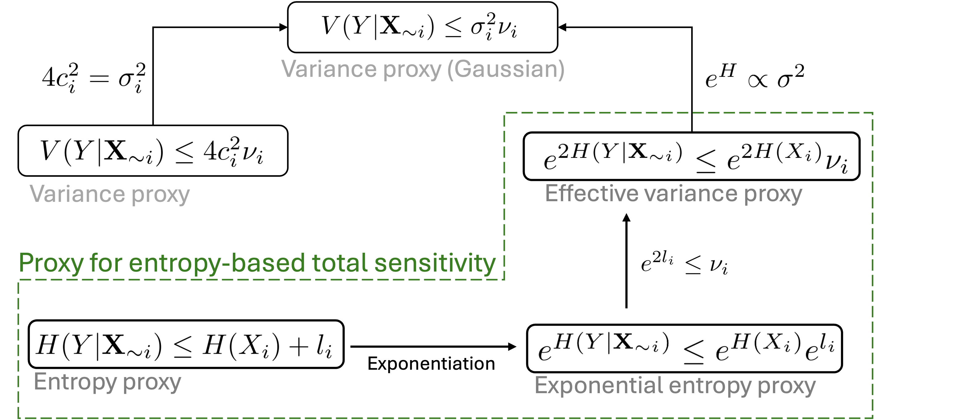
In addition, via exponentiation, we extend the upper bound to DGSM for a total sensitivity measure based on exponential entropies and exponential powers (also known as effective variance). In the special case with Gaussian inputs and linear functions, the proposed new proxy for entropy GSA is found to be equivalent to the proxy for variance-based total effect sensitivity. The detail of the above mentioned relationship between entropy and variance proxies are given in Section 3 and is summarised in Figure 1 for an overview.
.
In this paper, we focus on entropy-based GSA. However, it should be noted that there are many other moment-independent sensitivity measures [10], which are often based on a distance metric to measure the discrepancy between the conditional and unconditional output probability density functions (PDFs). For example, sensitivity indices based on the modification of the input PDFs have been proposed in [11] for reliability sensitivity analysis, where the input perturbation is derived from minimizing the probability divergence under constraints. [12] proposed a moment independent -indicator that looks at the entire input/output distribution. The definition of -indicator examines the expected total shift between the conditional and unconditional output PDFs, where the shift is conditional on one or more of the random input variables. Recently, the Fisher Information Matrix has been proposed to examine the perturbation of the entire joint probability density function (jPDF) of the outputs, and is closely linked to the relative entropy between the jPDF of the outputs and its perturbation due to an infinitesimal variation of the input distributions [13, 14].
In what follows, we will first review global sensitivity measures in Section 2, where the motivation for the entropy-based measure and its proxy is discussed with an example. In Section 3, we establish the inequality relationship between the total effect entropy measure and the partial derivatives of the function of interest, where mathematical proofs and numerical verifications are provided. In Section 4, we demonstrate the advantages of exponential entropy as a sensitivity measure and discuss its link with variance-based indices and their proxy. Concluding remarks are given in Section 5.
2 Global sensitivity measures
This research is motivated by applications of global sensitivity analysis (GSA) towards mathematical models. Such problems are common in computer experiments, where a physical phenomenon is studied with a complex numerical code and GSA is employed to better understand how they work, reduce the dimensionality of the problem, and help with calibration and verification [15]. In this context, an important question for GSA is: ‘Which model inputs can be fixed anywhere over its range of variability without affecting the output?’ [2]. In this section, we first review both variance-based and derivative-based sensitivity measures, which can provide answers to the above ‘screening’ question. After discussing the links between the two measures, we will use a simple example to motivate the use of entropy-based sensitivity indices.
2.1 Total effect sensitivity and its link with derivative-based measures
The variance-based total effect measure accounts for the total contribution of an input to the output variation, and is often a preferred approach due to its intuitive interpretation and quantitative nature.
Let us denote as independent random input variables, and being the output of our computational model represented by a function , such that .
The variance-based GSA decompose the output variance into conditional terms [2]:
| (1) |
where
and so on for the higher interaction terms. measures the first order effect variance and for a second order effect variance, where their contributions to the unconditional model output variance can be quantified as and respectively. Analogous formulas can be written for higher-order terms, enabling the analyst to quantify the higher-order interactions.
The total order sensitivity index is then defined as:
| (2) |
where is the set of all inputs except . The total order sensitivity index measures the total contribution of the input to the output variance, including its first order effect and its interactions of any order with other inputs.
The most direct computation of is via Monte Carlo (MC) estimation because it does not impose any assumption on the functional form of the response function. Various estimators for have been developed where the main difference is in the sampling design. A recent paper on comparing performance of several existing total-order sensitivity estimators can be found in [16]. Regardless of the specific estimator chosen, the computational cost for is a least , where is base sample number. Large values of , normally in the order of thousands or tenths of thousands, is needed for more accurate estimate of , and the computational cost has been noted as one of the main drawbacks of the variance-based GSA in [2].
The elementary effect method, also known as Morris’ method [2, 4], on the other hand is a simple and effective screening method for GSA. The Morris’ method is based on the construction of trajectories in the sampling space and the total cost of computation is . is typically between 10 and 50 [17], as compared to which is in the order of thousands for the estimation of .
When the function is differentiable, functionals based on have been proposed to examine the global sensitivity with respect to the parameter . The modified Morris sensitivity index [17] is an approximation of the following functional:
| (3) |
for and is the joint probability density function (jPDF) of . It has been empirically demonstrated in [17] that for some practical problems is similar to the variance-based total index .
Based on that observation, the Derivative-based Global Sensitivity Measure (DGSM):
| (4) |
has been proposed to be used as a proxy for [7, 8]. In particular, the total sensitivity variance is upper bounded by DGSM via the following inequality:
| (5) |
which is developed in [8] for random inputs with log-concave distributions such as exponential, beta and gamma distributions. is called the Cheeger constant. Although the Cheeger constant has no analytical expressions for general log-concave measures, it can be estimated numerically using the distribution function of the uncertain input as shown in [8].
2.2 A motivating example and entropy-based sensitivity
It has been pointed out in [18] that a major limitation of variance-based sensitivity indices is that they implicitly assume that output variance is a sensible measure of the output uncertainty, which might not always be the case. For instance, if the output distribution is multi-modal or if it is highly skewed, using variance as a proxy of uncertainty may lead to contradictory results.
To illustrate this point, we look at the simple function . In this case, the two inputs both follow the chi-squared distribution with and , and are assumed to be independent. This results in a positively skewed distribution of with a heavy tail. This example has been used in [19] to show that variance-based sensitivity indices fail to properly rank the inputs of a model whose output has a highly skewed distribution.
To overcome this issue, a Kullback-Leibler (KL) divergence based metric has been proposed in [19]:
| (6) |
where and are the probability density function of the output, depending on whether is fixed, usually at its mean. The larger the , the more important is. It was found in [19] that the effect of is higher in terms of divergence of the output distribution, but the variance-based total index shows that and are equally important. The higher influence of has also been confirmed in [18] where the sensitivity is characterised by the change of cumulative distribution function of the output.
Variance-based total index K-L divergence based index Derivative-based DGSM Entropy-based total index Variable 0.546 0.1571 8.4e-3 0.510 0.547 0.0791 2.1e-2 0.213
We reproduce the sensitivity results of and in Table 1 from [19]. In comparison, we have also computed the DGSM results, using numerical integrations as the derivatives are analytically available for this simple function. It can be seen from Table 1 that DGSM also provides misleading results in this case.
In addition, we also compare the results with the entropy-based total sensitivity index [20]:
| (7) |
where the average is calculated over all possible values of and is the differential entropy, e.g. . measures the remaining entropy of if the true values of can be determined, in analogy to the variance-based total effect index . Note that because [21].
has been estimated numerically based on the histogram method given in Appendix A, where samples are used. It can be seen from Table 1 that the entropy-based is able to effectively identify the higher influence of for this example. Note that different from which is conditional on the value of , for example are set at their mean values in Table 1, is an un-conditional sensitivity measure as all possible values of the inputs are averaged out.
We note in passing that analogously to the variance based sensitivity indices, a first order entropy index can also be defined as [22]. is the mutual information which measures how much knowing reduces uncertainty of or vice versa. The index can thus be regarded as a measure of the excepted reduction in the entropy of of by fixing .
2.3 Summary
From the motivating example, it became clear that variance-based total sensitivity index might provide misleading sensitivity results, due to the fact that only the second moment is considered. This is especially the case for highly skewed or multi-modal distributions . This limitation is overcome by the entropy-based measures which are applicable independent of the underlying shape of the distribution.
However, the entropy-based indices have limited application in practice, mainly due to the heavy computational burden where the knowledge of conditional probability distributions are required. Both histogram and kernel based density estimation methods have computational challenges for entropy-based sensitivity indices as pointed out in [18]. For example, it was noted in [3] that although both variance-based and entropy-based sensitivity analysis take long computational time, the convergence for conditional entropy estimation is even slower.
Motivated by the above issues and inspired by the low-cost sensitivity proxy for variance-based measures, the objective of this paper is to find a computational efficient proxy for entropy-based total sensitivity measure. An overview of the entropy proxies is summarised in Figure 1, while detail for their derivation is given in Section 3. For ease of reference, the main sensitivity measures considered in this paper are listed in Table 2.
Category Notation Description Derivative-based GSA measure Limiting value of the modified Morris index Derivative-based global sensitivity measure (DGSM) Log-derivative sensitivity measure Variance-based GSA measure Total effect variance Variance-based total effect index Entropy-based GSA measure Total effect entropy Entropy-based total effect index Total effect exponential entropy Exponential entropy based total effect index
3 Link between the partial derivatives and the total effect entropy measure
In this section, the relationship between the function partial derivatives and entropy-based sensitivity indices is explored. We will first establish the link in Section 3.1 and provide numerical verifications in Section 3.2 and 3.3.
Note that in this section we will consider the function where the function is differentiable. Recall that our interest here is for applications of global sensitivity analysis (GSA) towards mathematical models, where a physical phenomenon is typically studied with a complex numerical code. The computation of the partial derivatives can then be obtained via the companion adjoint code, or numerically estimated by a finite difference method. For example, the derivative-based DGSM can be estimated by finite difference, and this can be performed efficiently via Monte Carlo sampling as discussed in [5].
3.1 An upper bound for the total effect entropy
Let be a continuous random variable with the probability density function (PDF) given by . can be regarded as a transformed variable and the transformed PDF can then be found via the Jacobian matrix for the calculation of its differential entropy .
For a general vector transformation , the corresponding differential entropy are related as [23]:
| (8) |
where is the Jacobian matrix with and is the joint probability density function (jPDF) of . The above inequality becomes an equality if the transform is a bijection, i.e. an invertible transformation. Note that we have not assumed independent inputs for the inequality above.
As show in [23], Eq 8 can be proved substituting the transformed PDF into the expression of and note there will be a reduction of entropy if the transformation is not one-to-one. Following this line of thought, it was noted in [24] that Eq 8 can also be seen as one version of the data processing inequality, where the transformation does not increase information.
Now set where , and introduce dummy variables with . In this setting, the Jacobian matrix from the 2nd row onwards, i.e. , when and when . Therefore, the Jacobian matrix in this case is a triangular matrix. As a result, the Jacobian determinant is the product of the diagonal entries:
| (9) |
On the left hand side of the above inequality, the joint entropy of can be expressed using the conditional entropies as [21]. The subscript indicates the index ranging from to . On the right hand side of Eq 10, we have using the subadditivity property of the joint entropy of the input variables. The joint entropy becomes additive if the input variables are independent.
Putting these together, the inequality of Eq 10 then becomes:
where the expectation is with respect to the jPDF of the input variables. Note that is the expected conditional entropy.
The reasoning above uses the first variable as an example. However, the results hold for any variables via simple row/column exchanges, which only affects the sign of the determinant but not its modulus.
Therefore, we have the following equality:
| (11) |
where indicates the index ranges from to excluding , and we have introduced the following notation .
The conditional entropy measures the remaining entropy of if the true values of can be determined, in analogy to the total effect index from variance-based indices. Note that the conditional entropy is a global measure of uncertainty as the expectation is with respect to all possible values of .
The above inequality thus demonstrates that, for a differentiable function , the entropy-based total sensitivity is bounded by the expectation of log partial derivatives of the function, with the addition of the entropy of the input variable of interest. And this inequality becomes an equality if the input variables are independent and the transformation is bijection, i.e. is an invertible transformation and it has a unique inverse.
The inequality in Eq 11 is one of the main contributions of this paper. It establishes an upper bound for the total effect entropy using computationally efficient partial-derivative based functionals. As smaller tends to indicate smaller total effect entropy, it can thus be used to screen uninfluential variables and work as a low cost proxy for entropy-based indices.
The use of as a proxy for the total effect entropy is similar to the DGSM-based upper bound for the variance-based described in Eq 5. However, there is a major issue with the inequality in Eq 11: we cannot normalise Eq 11 by to obtain a bound on the entropy-based total effect indices , as can potentially be negative. In Section 4, we will overcome this issue by taking the exponentiation of the inequality in Eq 11, and demonstrate that the exponential entropy based measure has a more intuitive sensitivity interpretation and is closely linked to the variance-DGSM proxy. Before that, we will first verify Eq 11 using several examples in the next two subsections.
3.2 Examples - monotonic functions
We will first test monotonic functions where the equality of Eq 11 is expected, and examine the inequality with more general functions in the next section. All input variables are assumed to have the same uniform distribution for examples 1 - 4, i.e. , while Gaussian distributions are used for example 5. For verification purposes, all the examples in this section are chosen to have tractable expressions for both the integral of derivatives and the conditional entropies. Note that for simplicity the input variables are assumed to be independent in these numerical examples. Although input independence is required for the equality condition, the inequality in Eq 11 makes no assumptions of independence or distribution type for .
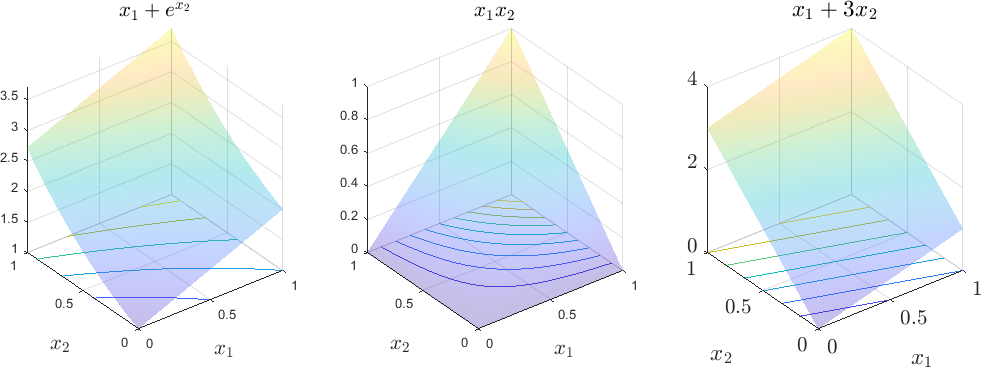
We can see below that for example 1 - 5 and that numerically verifies the equality case for Eq 11. For examples 1 - 3, the conditional entropies are also numerically estimated using the method given in Appendix A. This is to demonstrate that although numerical estimation of the total effect entropy can be conducted for the low dimensional problem, it can be computationally very expensive which is prohibitive for complex models.
Number of Samples 1.00E+03 0.0934 0.5251 -0.9057 -0.8468 0.2279 1.1269 1.00E+04 0.0602 0.5225 -0.9111 -0.9211 0.1043 1.1093 1.00E+05 0.0315 0.5131 -0.9528 -0.9593 0.0526 1.1047 1.00E+06 0.0148 0.5069 -0.9760 -0.9755 0.0242 1.1019 1.00E+07 0.0068 0.5034 -0.9879 -0.9878 0.0113 1.1000 1.00E+08 0.0032 0.5015 -0.9939 -0.9939 0.0052 1.0993 Exact results 0.0000 0.5000 -1.0000 -1.0000 0.0000 1.0986 error - -0.30% 0.61% 0.61% - -0.06% 0.0000 0.5000 -1.0000 -1.0000 0.0000 1.0986
Example 1.
For variable , because the differential entropy remains constant under addition of a constant ( is a constant for ). For right hand side of the inequality in Eq 11, we have , so .
For variable , , where is the conditional PDF of because the transformed variable has a PDF . Similarly, we have , so , which proves the equality as expected.
Example 2.
Consider the function , where the partial derivatives are and . For , the expected value are for both and . Recall that the differential entropy increases additively upon multiplication with a constant,. Same results can be obtained for due to the symmetry between and . Therefore, as given by Eq 11.
Example 3.
Consider the function , where the partial derivatives are 1 and 3 for and respectively. For , the expected value can be integrated analytically as 0 and respectively. It is straightforward to show that, as in previous examples, and , which is the same as .
Example 4.
Consider the product function , where (for , we recover the function in example 2). For , it is straightforward to show that and .
For variable , , which is the same as .
For variable , , where the conditional PDF of is because the transformed variable has a PDF . This is the same as .
Example 5.
This linear function, , has been used in [22] to demonstrate the equivalence between entropy based and variance based sensitivity indices for Guassian random inputs, i.e. . In the case with independent inputs, the sensitivity index based on the conditional entropy can be obtained as , and this is just the logarithmically scaled version of , i.e. . As for this simple linear function, the special equality case is obtained for the inequality given in Eq 11.
3.3 Examples - General functions
Both Ishigami function and G-function are commonly used test functions for global sensitivity analysis, due to the presence of strong interactions. These two functions, each with three input variables, are used in this section to demonstrate the inequality relationship derived in Eq 11. We will focus on the verification of Eq 11 in this section, but will re-visit these two functions in the next section for a discussion in comparison with variance-based sensitivity indices.
The conditional entropies are estimated numerically using Monte Carlo sampling as described in Appendix A. Different numbers of samples are used, ranging from to . For each estimation, the computation is repeated 20 times and both the mean value and the standard deviation (std) are reported in Table 4 and 5. For the estimation of derivative-based , Matlab’s inbuilt numerical integrator "integral" is used with the default tolerance setting.
Example 6.
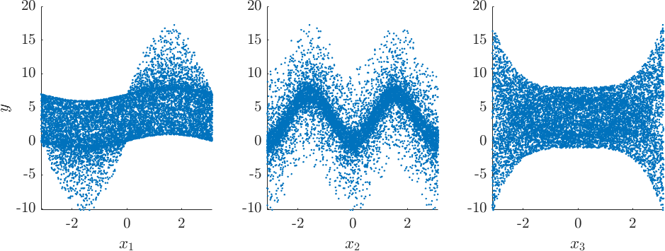
The Ishigami function, , is often used as an example for uncertainty and sensitivity analysis. It exhibits strong nonlinearity and nonmonotonicity, as can be seen in Figure 3a. In this case, and are used, and the input random variables have uniform distributions, i.e., for .
The sensitivity results are listed in Table 4, where it is clear that inequality from Eq 11 is satisfied. The total effect entropy is estimated with different numbers of samples, and each estimation with 20 repetitions for variability assurance. It is clear from the small std that the variation is small. However, the convergence of conditional entropy estimation is slow as large number of samples is needed, as we saw in Table 3.
Ishigami function Number of Samples mean std mean std mean std 1.00E+06 1.3902 0.0007 1.7614 0.0006 0.9701 0.0013 1.00E+07 1.2978 0.0003 1.7023 0.0001 0.7693 0.0004 1.00E+08 1.2335 0.0001 1.6609 0.0001 0.6066 0.0002 1.2335 1.6609 0.6066 1.9024 3.0906 0.6626
Example 7.
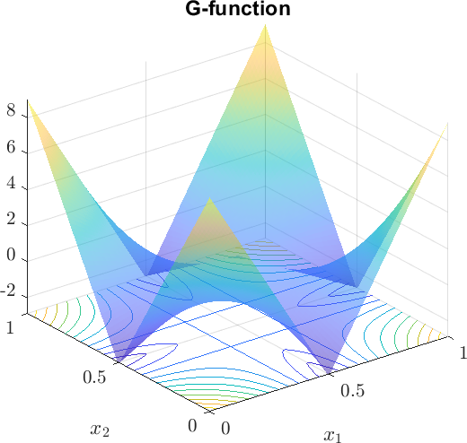
Consider the so-called G-function, , which is often used for numerical experiments in sensitivity analysis. It is a highly nonlinear function, as can be seen in Figure 3b for a two-variable example. In this case, , for . The input random variables have uniform distributions, i.e., for . A lower value of indicates a higher importance of the input variable , i.e., is the most important, while is the least important in this case. The sensitivity results for the G-function, in the same format as Table 4, are reported in Table 5. It is clear that the inequality relationship in Eq 11 is satisfied.
G-function with Number of Samples mean std mean std mean std 1.00E+06 0.3477 0.0009 -0.1376 0.0013 -0.3988 0.0015 1.00E+07 0.3398 0.0006 -0.1737 0.0005 -0.4482 0.0006 1.00E+08 0.3378 0.0003 -0.1917 0.0002 -0.4738 0.0002 0.3378 -0.1917 -0.4738 1.3863 0.9808 0.6931
4 Exponential entropy based total sensitivity measure
There are two issues with the differential entropy based sensitivity measure: 1) as pointed out in [20], entropy for continuous random variables (aka differential entropy) can become negative and this is undesirable for sensitivity analysis. More importantly, as mentioned in Section 3.1, the inequality in Eq 11 is not valid when normalised by a negative ; 2) the interpretation of conditional entropy is not as intuitive as variance based sensitivity indices. This is partly due to the fact that variance-based methods is firmly anchored in variance decomposition, but also because entropy measures the average information or non-uniformity of a distribution as compared to variance which measures the spread of data around the mean. Although non-uniformity can be seen as a suitable measure for epistemic uncertainties [22], its interpretation for GSA in a general setting can be further improved.
We propose to use exponential entropy as a entropy-based measure for global sensitivity analysis, to overcome these two issues. Studies in [3] already noted that an exponentiation of the standard entropy-based sensitivity measures may improve its discrimination power. We take an exponentiation of the inequality in Eq 11:
| (12) |
where we recall that . Divide both sides of Eq 12 by :
| (13) |
where can be considered as the exponential entropy based total sensitivity indices, and the upper bound can then used as a proxy for . As , so we have which is desirable as sensitivity indices.
In addition, and the un-normalised have a more intuitive interpretation as GSA indices as compared to the standard differential entropy, because exponential entropy can be seen as a measure for the effective spread or extent of a distribution [6].
4.1 Intuitive interpretation of sensitivity based on exponential entropy
To explain this point, we first recall that the entropy of a random variable with a uniform distribution is , where are the bounds of the distribution. Taking the natural exponentiation of the entropy in this case results in , which is the range of the uniform distribution. For a Gaussian distribution with variance , the exponential entropy is which is proportional to the variance.
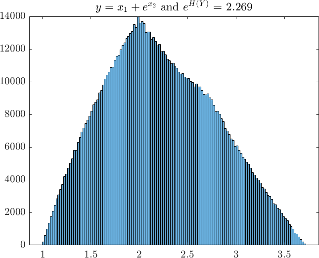
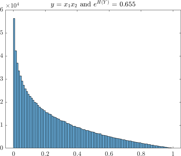
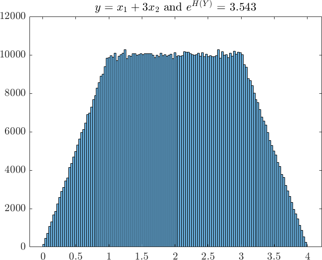
This becomes more evident if we plot the histogram of function output from examples 1 to 3 in Figure 4. These histograms are based on Monte Carlo samples and from which we have calculated the exponential entropy for each case. When compared to the range of the distribution, the values of the exponential entropy provide intuitive indication of the spread of the distribution, in analogy to standard deviation or variance. For example, the average width of the top and bottom of the trapezium in Example 3 is approximately , which is about the same as the exponential entropy of .
Therefore, the exponential entropy can be regarded as a measure of the extent, or effective support, of a distribution and this has been discussed in details in [6]. As measures the remaining entropy in average if the true values of can be determined, the exponentiation of the conditional entropy, , can thus be regarded as the effective remaining range of the output distribution conditioning on that are known. then measures the ratio of the effective range before and after are fixed, and larger thus indicate a higher influence of .
4.2 Link between exponential entropy and variance
Last but not least, in addition to its non-negativity and a more intuitive interpretation for GSA, exponential entropy is also closely linked to variance-based GSA indices and their corresponding bounds. To demonstrate this, we first note that the three different derivative-based sensitivity indices listed in Table 2 are closely related as:
| (14) |
where it is evident that based on Cauchy-Schwarz inequality. In addition, we have using Jensen’s inequality as the exponential function is convex. So the inequality for the exponential entropy in Eq 12 can be further extended to:
| (15) |
where we recall that is the derivative-based DGSM indices.
Eq 15 already looks remarkably similar to the variance-DGSM inequality given in Eq 5. In fact, the squared exponential entropy of a random variable , also called entropy power, is known from information theory to be bounded by the variance of with [21], where the equality is obtained if is a Gaussian random variable. Therefore, for independent Gaussian inputs with variance , we have . The squared exponential entropy thus measures the ‘effective variance’ as it is simply the variance of a Gaussian random variable with the same entropy [25].
In the special case where the function is a linear function, the conditional distribution of is also Gaussian, and it indicates that the conditional entropy power would also be proportional to the conditional variances of the output, i.e. (cf Example 5 in Section 3). Therefore, it is clear that with independent Gaussian inputs and a linear function, we have from Eq 15:
| (16) |
which indicates that in this special case the entropy-DGSM bound from Eq 15 is equivalent to the variance-DGSM relationship given in Eq 5.
4.3 Examples with Ishigami function and G-function
In this section, we will revisit the Ishigami function of Example-6 and G-function of Example-7 from Section 3.3 using the exponential entropy based total sensitivity index . The results of are listed in Table 6. They are obtained using the mean values of the total effect entropy from Table 4 and 5 with samples, and the corresponding for the output.
G-function 0.5306 0.3125 0.2357 0.6246 0.3240 0.1913 Ishigami 0.2300 0.3527 0.1229 0.5576 0.4424 0.2437
In comparison, we have also calculated the variance based , using samples with 20 repetitions. The mean values for are listed in Table 6. It can be seen that the results from are generally consistent with , especially for G-function where the sensitivity ranking are similar both qualitatively and quantitatively. For the Ishigami function, both indices have successfully identified the contribution of which is the lowest. However, the relative importance of and are opposite from and . This difference between variance-based and entropy-based ranking for Ishigami function was also noted in [3], but without further explanation.
We attempt to look at the difference using a simple function with as the input random variables:
| (17) |
which can be seen to represent the interaction effect of and in the Ishigami function. The conditional variance and entropy of are thus:
| (18) |
where the translation invariance of variance and entropy are used. And the corresponding un-conditional and can be found as:
| (19) |
From 19, it is clear that despite the similarities, the conditional variance depends on which grows much faster than for the conditional entropy as increases.
In the Ishigami function, the effect of grows fast as approach its boundary, i.e. towards and . This is evident from the scatter plot of for in Figure 3a. The much stronger interaction at the support boundary between and has also been noted in [26], where the importance of was found to be much reduced if the support of the distribution of is reduced by percent. Putting would put as the most influential variable.
From Eq 19, we can see that the interaction between and is more influential for the conditional variance due to the squaring effect, as compared to the entropy operation which takes logarithm of the interaction. This difference increases towards the boundary as the interaction between and gets stronger towards and . And this helps to explain why is the most influential variable for the variance-based . This example highlights that, despite many similarities, entropy and variance are fundamentally different, for example, the variable interactions are processed differently between them.
5 A flood model case study
The motivation of this paper is to identify a much more computational efficient proxy for entropy-based total effect sensitivity. has been proved to upper bound the total effect exponential entropy, thus, can be used as a proxy for and its normalised version as a proxy for .
We have demonstrated the inequality via several numerical examples in Section 3 for the differential entropy based measure. In the previous section, the use of the log-derivative has been further extended to the more commonly used DGSM indices , where can be used as a proxy for . This is especially useful when are known.
To illustrate this point for practical problems, a simple river flood model is considered where has been used for sensitivity analysis. This model has been used in [8] for demonstration of the use of Cheeger constant for factor prioritization with DGSM, and as an example in GSA review [27].
This model simulates the height of a river, and flooding occurs when the river height exceeds the height of a dyke that protects industrial facilities. It is based on simplification of the 1D hydro-dynamical equations of SaintVenant under the assumptions of uniform and constant flow rate and large rectangular sections. The quantity of interest in this case is the maximal annual overflow :
| (20) |
where the distributions of the independent input variables are listed in Table 7. We have also added the exponential entropy value for each variable in Table 7. The analytical expressions for differential entropy of most probability distributions are readily available and well documented. A comprehensive list can be found in [28].
For a truncated distribution with the interval , its differential entropy can be found as [29]:
| (21) |
where and are the original probability density function (PDF) and cumulative distribution function (CDF) of the random variable respectively. is the PDF of the truncated distribution where . As both and are analytically known, Eq 21 can then integrated numerically for the truncated entropy.
Variable Description Distribution Function Exponential Entropy Maximal annual flowrate [m3/s] Truncated Gumbel (1013,558) on [500,3000] 2051 Strickler coefficient [ - ] Truncated Normal (30,8) on [15, ] 30 River downstream level [m] Triangular (49,50,51) 1.65 River upstream level [m] Triangular (54,55,56) 1.65 Dyke height [m] Uniform [7,9] 2 Bank level [m] Triangular (55,55.5,56) 0.825 Length of the river stretch [m] Triangular (4990,5000,5010) 16.5 River width [m] Triangular (295,300,305) 8.24
The results for the sensitivity indices are shown in Table 8, where both the variance-based and derivative-based results are obtained from Table 5 of reference [8]. According to [8], the variance-based index is based on model evaluations, while a Sobol’ sequence is used with model evaluations for estimating the derivative-based DGSM. Note that different from [8], the un-normalised total effect variance and its DGSM based upper bound are given in Table 8. Recall that and variance of the output in this case.
Also given in Table 8 is the entropy-based upper bound, which is calculated using the exponential entropy values listed in Table 7 and the results. Note that as analytical expressions are typically available for entropy, there is negligible extra cost for the estimation the entropy-DGSM upper bound once are known. From the entropy-DGSM proxy, we can see that four input variables, , have been identified as the most important variables for maximal annual overflow, with and of negligible influence.
In comparing the new entropy-DGSM proxy with results from other measures, it is clear from Table 8 that: 1) DGSM alone failed to properly rank the input variables in this case, as pointed out in [8]. We can get a hint for the reason from Eq 11 where it is clear that, although is a global measure, it is the combination of and the derivative-based that has the direct link with the total entropy effect. This point is also reflected in the variance proxy where is scaled by the Cheeger constant which is a function of the distribution functions of the inputs; 2) Both upper bound proxies, entropy-based and variance-based , provide consistent results as compared to the total effect variance ; 3) The entropy-DGSM upper bound outperforms the variance-DGSM proxy, by ranking the variables in exactly the same order as the total effect variance. Note that the order of and is negligible as their influence is almost zero.
It is thus clear that the entropy-DGSM upper bound can be used as a proxy for the total effect sensitivity analysis. As compared to the Cheeger constant, the normalization constant is also easier to compute as the entropy of many distribution functions are known in closed form. The main computational cost for estimation of the entropy-DGSM proxy is thus for the calculation , which is much more affordable than the estimation of the conditional variance or the conditional entropy.
Total effect variance Derivative-based DGSM Variance-DGSM Upper Bound Entropy-DGSM Upper Bound Variable 0.414 (1) 1.296e-06 (7) 3.295 (1) 5.452 (1) 0.163 (4) 3.286e-03 (5) 0.233 (4) 2.960 (4) 0.218 (3) 1.123e+00 (1) 0.659 (2) 3.053 (3) 0.004 (6) 2.279e-02 (4) 0.013 (6) 0.062 (6) 0.324 (2) 8.389e-01 (2) 0.399 (3) 3.356 (2) 0.042 (5) 8.389e-01 (3) 0.123 (5) 0.570 (5) 0.000 (7) 2.147e-08 (8) 0.000 (7) 0.000 (8) 0.000 (8) 2.386e-05 (6) 0.000 (8) 0.002 (7)
6 Conclusions
A novel global sensitivity proxy for entropy-based total effect has been developed in this paper. This development is motivated by the observation that, on the one hand, for distributions where the second moment is not a sensible measure of the output uncertainty such as highly skewed distributions, entropy-based sensitivity indices can perform better for global sensitivity analysis than variance-based measures. It is also driven by the issue that, on the other hand, entropy-based indices have limited application in practice, mainly due to the heavy computational burden where the knowledge of conditional probability distributions are required.
We have made use of the inequality between the entropy of the model output and its inputs, which can be seen as an instance of data processing inequality, and established an upper bound for the total effect entropy . This upper bound is tight for monotonic functions and this has been demonstrated numerically. Extending to general functions, the upper bound was able to provide similar input rankings and thus can be regarded as a proxy for entropy-based total effect measure. Applying to a physics model for flood analysis, the new proxy shows much improved variable ranking capability compared to derivative-based global sensitivity measures (DGSM).
The resulted proxy is based on partial derivatives and thus computationally cheap to estimate. If the the derivatives are available, e.g. as output of a computational code, the proxy would be readily available. Even if a Monte Carlo based approach is used, the computational cost is typically in the order or , as compared to for entropy-based indices. This computational advantage is why derivative-based methods, such as the Morris’ method and DGSM, are popular among practitioners whenever computational cost is of major concern. This is especially true for high dimensional problems, where it becomes infeasible to estimate conditional entropies as many instances of conditional distributions are required.
Drawing on the criticism of using differential-entropy as sensitivity indices, we propose to use its exponentiation which is both non-negative and offer a more intuitive interpretation as sensitivity indices. The total effect exponential entropy and its normalised indices measure the effective remaining extent or spread of a distribution conditioning on that are known. Larger or thus indicate a higher influence of . This interpretation is similar to the variance-based sensitivity indices as variance is also a measure of distribution spread. However, entropy-based and variance-based indices are fundamentally different and they would generally provide different variable ranking. This is evident from the Ishigami function example where it was found that the interaction effect between variables are processed differently.
The sensitivity measure based on exponential entropy is mainly introduced in this work for the purpose of extending the conditional entropy upper bound. However, is interesting in its own right, as it possesses many desirable properties for GSA, such as quantitative, moment independent and easy to interpret. The G-function example in Section 4.3 shows that is close to one for this product function, as opposed to the variance-based indices where the sum of sensitivity indices is equal to one for additive functions. As exponential entropy can be seen as a geometric mean of the underlying distribution, i.e. , one of the future research is to examine the unique properties of GSA indices based on exponential entropy, and explore its decomposition characteristics for sensitivity analysis of different interaction orders.
Acknowledgment
For the purpose of open access, the author has applied a Creative Commons Attribution (CC BY) licence to any Author Accepted Manuscript version arising.
Data availability statement
The authors confirm that the data supporting the findings of this study are available within the article.
References
- [1]
- [2] Saltelli, A.: Global sensitivity analysis: the primer. John Wiley, 2008 http://books.google.at/books?id=wAssmt2vumgC. – ISBN 9780470059975
- [3] Auder, B ; Iooss, B: Global sensitivity analysis based on entropy. In: Proceedings of the ESREL 2008 Conference (2008), S. 2107–2115
- [4] Morris, Max D.: Factorial Sampling Plans for Preliminary Computational Experiments. In: Technometrics 33 (1991), Nr. 2, 161-174. http://dx.doi.org/10.1080/00401706.1991.10484804. – DOI 10.1080/00401706.1991.10484804
- [5] Kucherenko, S ; Rodriguez-Fernandez, María ; Pantelides, C ; Shah, Nilay: Monte Carlo evaluation of derivative-based global sensitivity measures. In: Reliability Engineering & System Safety 94 (2009), Nr. 7, S. 1135–1148
- [6] Campbell, L L.: Exponential entropy as a measure of extent of a distribution. In: Zeitschrift für Wahrscheinlichkeitstheorie und verwandte Gebiete 5 (1966), Nr. 3, S. 217–225
- [7] Sobol’, I.M. ; Kucherenko, S.: Derivative based global sensitivity measures and their link with global sensitivity indices. In: Mathematics and Computers in Simulation 79 (2009), Nr. 10, S. 3009–3017
- [8] Lamboni, M. ; Iooss, B. ; Popelin, A.-L. ; Gamboa, F.: Derivative-based global sensitivity measures: General links with Sobol’ indices and numerical tests. In: Mathematics and Computers in Simulation 87 (2013), 45-54. http://dx.doi.org/https://doi.org/10.1016/j.matcom.2013.02.002. – DOI https://doi.org/10.1016/j.matcom.2013.02.002. – ISSN 0378–4754
- [9] Wainwright, Haruko M. ; Finsterle, Stefan ; Jung, Yoojin ; Zhou, Quanlin ; Birkholzer, Jens T.: Making sense of global sensitivity analyses. In: Computers & Geosciences 65 (2014), 84-94. http://dx.doi.org/https://doi.org/10.1016/j.cageo.2013.06.006. – DOI https://doi.org/10.1016/j.cageo.2013.06.006. – ISSN 0098–3004. – TOUGH Symposium 2012
- [10] Borgonovo, Emanuele ; Plischke, Elmar: Sensitivity analysis: A review of recent advances. In: European Journal of Operational Research 248 (2016), Nr. 3, 869-887. http://dx.doi.org/https://doi.org/10.1016/j.ejor.2015.06.032. – DOI https://doi.org/10.1016/j.ejor.2015.06.032. – ISSN 0377–2217
- [11] Lemaître, P. ; Sergienko, E. ; Arnaud, A. ; Bousquet, N. ; Gamboa, F. ; Iooss, B.: Density modification-based reliability sensitivity analysis. In: Journal of Statistical Computation and Simulation 85 (2015), Nr. 6, 1200-1223. http://dx.doi.org/10.1080/00949655.2013.873039. – DOI 10.1080/00949655.2013.873039
- [12] Borgonovo, E.: A new uncertainty importance measure. In: Reliability Engineering & System Safety 92 (2007), Nr. 6, 771-784. http://dx.doi.org/https://doi.org/10.1016/j.ress.2006.04.015. – DOI https://doi.org/10.1016/j.ress.2006.04.015. – ISSN 0951–8320
- [13] Yang, Jiannan: A general framework for probabilistic sensitivity analysis with respect to distribution parameters. In: Probabilistic Engineering Mechanics 72 (2023), S. 103433
- [14] Yang, Jiannan: Decision-Oriented Two-Parameter Fisher Information Sensitivity Using Symplectic Decomposition. In: Technometrics 0 (2023), Nr. 0, 1-12. http://dx.doi.org/10.1080/00401706.2023.2216251. – DOI 10.1080/00401706.2023.2216251
- [15] Razavi, Saman ; Jakeman, Anthony ; Saltelli, Andrea ; Prieur, Clémentine ; Iooss, Bertrand ; Borgonovo, Emanuele ; Plischke, Elmar ; Piano, Samuele L. ; Iwanaga, Takuya ; Becker, William u. a.: The future of sensitivity analysis: an essential discipline for systems modeling and policy support. In: Environmental Modelling & Software 137 (2021), S. 104954
- [16] Puy, Arnald ; Becker, William ; Piano, Samuele L. ; Saltelli, Andrea: The battle of total-order sensitivity estimators. In: arXiv preprint arXiv:2009.01147 (2020)
- [17] Campolongo, Francesca ; Cariboni, Jessica ; Saltelli, Andrea: An effective screening design for sensitivity analysis of large models. In: Environmental modelling & software 22 (2007), Nr. 10, S. 1509–1518
- [18] Pianosi, Francesca ; Wagener, Thorsten: A simple and efficient method for global sensitivity analysis based on cumulative distribution functions. In: Environmental Modelling & Software 67 (2015), S. 1–11
- [19] Liu, Huibin ; Chen, Wei ; Sudjianto, Agus: Relative entropy based method for probabilistic sensitivity analysis in engineering design. In: Journal of Mechanical Design 128 (2006), Nr. 2, S. 326–336
- [20] Kala, Zdeněk: Global sensitivity analysis based on entropy: From differential entropy to alternative measures. In: Entropy 23 (2021), Nr. 6, S. 778
- [21] Cover, Thomas M.: Elements of information theory. John Wiley & Sons, 1999
- [22] Krzykacz-Hausmann, Bernard: Epistemic sensitivity analysis based on the concept of entropy. In: Proceedings of SAMO2001 (2001), S. 31–35
- [23] Papoulis, Athanasios: Probability, random variables and stochastic processes. 1984
- [24] Geiger, Bernhard C. ; Kubin, Gernot: On the information loss in memoryless systems: The multivariate case. In: arXiv preprint arXiv:1109.4856 (2011)
- [25] Costa, Max ; Cover, Thomas: On the similarity of the entropy power inequality and the Brunn-Minkowski inequality (corresp.). In: IEEE Transactions on Information Theory 30 (1984), Nr. 6, S. 837–839
- [26] Fruth, Jana ; Roustant, Olivier ; Kuhnt, Sonja: Support indices: Measuring the effect of input variables over their supports. In: Reliability Engineering & System Safety 187 (2019), S. 17–27
- [27] Iooss, Bertrand ; Lemaître, Paul: A review on global sensitivity analysis methods. In: Uncertainty management in simulation-optimization of complex systems: algorithms and applications (2015), S. 101–122
- [28] Lazo, A V. ; Rathie, Pushpa: On the entropy of continuous probability distributions (corresp.). In: IEEE Transactions on Information Theory 24 (1978), Nr. 1, S. 120–122
- [29] Moharana, Rajesh ; Kayal, Suchandan: Properties of Shannon entropy for double truncated random variables and its applications. In: Journal of Statistical Theory and Applications 19 (2020), Nr. 2, S. 261–273
- [30] Moddemeijer, Rudy: On estimation of entropy and mutual information of continuous distributions. In: Signal processing 16 (1989), Nr. 3, S. 233–248
Appendix A Numerical estimation of entropy
Adopting the approach from [30], the -plane is gridded by equal size cells () with coordinates (, ). The probability of observing a sample in cell (, ) is:
| (A.1) |
where is the centre of the cell.
Assuming the jPDF is approximately constant within a cell, the joint entropy can be represented as:
| (A.2) |
where represents the number of samples observed in the cell (, ), and is the total number of samples.
Similarly, the conditional entropy can be approximated as:
| (A.3) |
where and similar expressions can be derived when is a vector variable.