Depth-Centric Dehazing and Depth-Estimation from
Real-World Hazy Driving Video

Junkai Fan¹, Kun Wang¹, Zhiqiang Yan¹, Xiang Chen¹, Shangbing Gao², Jun Li¹ and Jian Yang¹¹¹footnotemark: 1 Corresponding authors

Abstract

In this paper, we study the challenging problem of simultaneously removing haze and estimating depth from real monocular hazy videos. These tasks are inherently complementary: enhanced depth estimation improves dehazing via the atmospheric scattering model (ASM), while superior dehazing contributes to more accurate depth estimation through the brightness consistency constraint (BCC). To tackle these intertwined tasks, we propose a novel depth-centric learning framework that integrates the ASM model with the BCC constraint. Our key idea is that both ASM and BCC rely on a shared depth estimation network. This network simultaneously exploits adjacent dehazed frames to enhance depth estimation via BCC and uses the refined depth cues to more effectively remove haze through ASM. Additionally, we leverage a non-aligned clear video and its estimated depth to independently regularize the dehazing and depth estimation networks. This is achieved by designing two discriminator networks: $D_{\text{MFIR}}$ enhances high-frequency details in dehazed videos, and $D_{\text{MDR}}$ reduces the occurrence of black holes in low-texture regions. Extensive experiments demonstrate that the proposed method outperforms current state-of-the-art techniques in both video dehazing and depth estimation tasks, especially in real-world hazy scenes. Project page: https://fanjunkai1.github.io/projectpage/DCL/index.html.

Introduction

Recently, video dehazing and depth estimation in real-world monocular hazy video have garnered increasing attention due to their importance in various downstream visual tasks, such as object detection (Hahner et al. 2021), semantic segmentation (Ren et al. 2018), and autonomous driving (Li et al. 2023). Most video dehazing methods (Xu et al. 2023; Fan et al. 2024) rely on a single-frame haze degradation model expressed through the atmospheric scattering model (ASM) (McCartney 1976; Narasimhan and Nayar 2002):

I(x)=J(x)t(x)+A_{\infty}(1-t(x)),

(1)

where $I(x)$ , $J(x)$ and $t(x)$ denote the hazy image, clear image and transmission map at a pixel position $x$ , respectively. $A_{\infty}$ represents the infinite airlight and $t(x)=e^{-{\beta(\lambda)}d(x)}$ with $d(x)$ as the scene depth and $\beta(\lambda)$ as the scattering coefficient for wavelength $\lambda$ . Clearly, $t(x)$ shows that ASM is depth-dependent, with improved depth estimation leading to better dehazing performance. Depth is estimated from real monocular hazy video using a brightness consistency constraint (BCC) between a pixel position $x$ in the current frame and its corresponding pixel position $y$ in an adjacent frame (Wang et al. 2021), that is,

y\sim KP_{x\rightarrow y}d(x)K^{-1}x,

(2)

where $K$ is the camera intrinsic parameter and $P_{x\rightarrow y}$ is the relative pose for the reprojection. This suggests that clearer frames contribute to more accurate depth estimation. These two findings motivate the integration of the ASM model with the BCC constraint into a unified learning framework.

Refer to caption — Figure 1: Visual comparisons of DVD (Fan et al. 2024), Lite-Mono (Zhang et al. 2023) and our DCL for dehazing and depth estimation in real-world hazy scenes.

In practice, while both ASM and BCC yield promising dehazing results and depth estimates on synthetic hazy videos (Xu et al. 2023; Gasperini et al. 2023), respectively, they often fall short in real-world scenes as it is difficult to capture accurately aligned ground truth due to unpredictable weather conditions and dynamic environments (Fan et al. 2024). For example, Fig.1 (b) shows the blurred depth obtained from the hazy video using Lite-Mono (Zhang et al. 2023). To improve dehazing performance, DVD (Fan et al. 2024) introduces a non-aligned regularization (NAR) strategy that collects clear non-aligned videos to regularize the dehazing network. However, DVD still produces dehazed frames with weak textures, causing blurred depth, in Fig. 1 (c).

Based on the above discussions, we propose a new Depth-Centric Learning (DCL) framework to simultaneously remove haze and estimate depth from real-world monocular hazy videos by effectively integrating the ASM model and the BCC constraint. First, starting with the hazy video frame, we design a shared depth estimation network to predict the depth $d$ . Second, we define distinct deep networks to compute adjacent dehazed frames $J_{x}$ and $J_{y}$ , the scattering coefficient $\beta$ , and the relative pose $P_{x\rightarrow y}$ , respectively. Moreover, dark channel (He, Sun, and Tang 2010) is used to calculate the $A_{\infty}$ value. Third, these networks are trained using the ASM model to reconstruct the hazy frame while the BCC constraint is employed to reproject pixels from $J_{x}$ to $J_{y}$ .

Inspired by the NAR strategy, we leverage a clear non-aligned video to estimate accurate depth using MonoDepth2 (Godard et al. 2019), thereby constraining both the dehazing and depth estimation networks. Specifically, we introduce a Misaligned Frequency & Image Regularization discriminator, $D_{\text{MFIR}}$ , which assists the discriminator network in constraining the dehazing network to recover more high-frequency details by utilizing frequency domain information obtained through wavelet transforms (Gao et al. 2021). Additionally, the accurate depth maps serve as references for Misaligned Depth Regularization discriminator $D_{\text{MDR}}$ , further mitigating issues such as black holes in depth maps caused by weak texture regions. Our contributions are summarized as follows:

•

To the best of our knowledge, we are the first to propose a Depth-centric Learning (DCL) framework that effectively integrates the atmospheric scattering model and brightness consistency constraint, enhancing both video dehazing and depth estimation simultaneously.
•

We introduce two discriminator networks, $D_{\text{MFIR}}$ and $D_{\text{MDR}}$ , to address the loss of high-frequency details in dehazed images and the black holes in depth maps with weak textures, respectively.
•

We evaluate the proposed method separately using video dehazing datasets (e.g., GoProHazy, DrivingHazy and InternetHazy) (Fan et al. 2024) and depth estimation datasets (e.g., DENSE-Fog) (Bijelic et al. 2020) in real hazy scenes. The experimental results demonstrate that our method exceeds previous state-of-the-art competitors.

Related work

Image/video dehazing. Early methods for image dehazing primarily focused on integrating atmospheric scattering models (ASM) with various priors (He, Sun, and Tang 2010; Fattal 2014), while recent advances have leveraged deep learning with large hazy/clear image datasets (Li et al. 2018b; Fang et al. 2025). These approaches use neural networks to either learn physical model parameters (Deng et al. 2019; Li et al. 2021; Liu et al. 2022a) or directly map hazy to clear images/videos (Qu et al. 2019; Qin et al. 2020; Ye et al. 2022). However, they rely on aligned synthetic data, resulting in domain shifts in real-world scenarios. To address this, domain adaptation (Shao et al. 2020; Chen et al. 2021; Wu et al. 2023) and unpaired dehazing model (Zhao et al. 2021; Yang et al. 2022; Wang et al. 2024) are used for real dehazing scenes. Despite these efforts, image dehazing models still encounter brightness inconsistencies between adjacent frames when applied to videos, leading to noticeable flickering.

Video dehazing techniques leverage temporal information from adjacent frames to enhance restoration quality. Early methods focused on post-processing to ensure temporal consistency by refining transmission maps (Ren et al. 2018) and suppressing artifacts (Chen, Do, and Wang 2016). Some approaches also addressed multiple tasks, such as depth estimation (Li et al. 2015) and detection (Li et al. 2018a), within hazy videos. Recently, (Zhang et al. 2021) introduced the REVIDE dataset and a confidence-guided deformable network, while (Liu et al. 2022b) proposed a phase-based memory network. Similarly, (Xu et al. 2023) developed a memory-based physical prior guidance module for incorporating prior features into long-term memory. Although some image restoration methods (Yang et al. 2023) excel on REVIDE in adverse weather, they are mainly trained on indoor smoke scenes, limiting their effectiveness in real outdoor hazy conditions.

In contrast to previous dehazing and depth estimation works (Yang et al. 2022; Chen et al. 2023), our DCL is trained on real hazy video instead of synthetic hazy images. Furthermore, it simultaneously optimizes both video dehazing and depth estimation by integrating the ASM model with the brightness consistency constraint (BCC).

Self-supervised Monocular Depth Estimation (SMDE). Laser radar perception is limited in extreme weather, leading to a growing interest in self-supervised methods. Building on the groundbreaking work (Zhou et al. 2017), which showed that geometric constraints between consecutive frames can achieve strong performance, researchers have explored various cues for self-supervised training using video sequences (Godard et al. 2019; Watson et al. 2021; Liu et al. 2024) or stereo image pairs (Godard, Mac Aodha, and Brostow 2017). Recently, advanced networks (Zhang et al. 2023; Zhao et al. 2022) have been used for self-supervised depth estimation (SMDE) in challenging conditions like rain, snow, fog, and low light. However, degraded images, especially in low-texture areas, significantly hinder accurate depth estimation. To address this, some methods focus on image enhancement (Wang et al. 2021; Zheng et al. 2023) and domain adaptation (Gasperini et al. 2023; Saunders, Vogiatzis, and Manso 2023). While these methods improve depth estimation, they typically rely on operator-based enhancements rather than learnable approaches. Additionally, domain adaptation, often based on synthetic data, may not generalize well to real-world scenes.

Compared to the above SMDE methods, our approach leverages a learnable framework based on a physical imaging model, trained directly on real-world data. This approach effectively mitigates the domain gap, offering improved performance in real-world scenarios.

Methodology

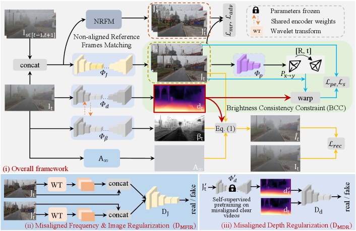
In this section, we propose a novel Depth-centric Learning (DCL) framework (see Fig. 2) to simultaneously remove haze and estimate depth from real-world monocular hazy videos. First, we introduce a unified ASM-BCC model that effectively integrates the ASM model and the BCC constraint. Next, we present two misaligned regularization discriminator networks, $D_{\text{MFIR}}$ and $D_{\text{MDR}}$ , for enhancing constraints on high-frequency details and weak texture regions. Finally, we outline the overall training loss.

A Unified ASM-BCC Model

For a given hazy video clip with a current frame $I_{t}$ and its adjacent frames, $I_{s\in[t-n:t+n],s\neq t}\in\mathbb{R}^{3\times h\times w}$ , where $h$ is the height, $w$ is the width and we set $n=1$ , we define a unified ASM-BCC model by combining Eqs. (1) and (2):

\displaystyle\left\{\begin{array}[]{ll}I_{t}(x)=J_{t}(x)e^{-{\beta}\textbf{d(x)}}+A_{\infty}\left(1-e^{-{\beta}\textbf{d(x)}}\right)\\ J_{t}(x)=\mathcal{S}(J_{s},y),\ y\sim KP_{x\rightarrow y}\textbf{d(x)}K^{-1}x\\ \end{array}\right.

(5)

where $J_{s}$ is a dehazed frame computed by the dehazing network from the hazy frame $I_{s}$ . The function $\mathcal{S}$ denotes the differentiable bilinear sampling operation (Jaderberg et al. 2015), $x$ and $y$ represent the pixel positions of the frames $I_{t}$ and $I_{s\in[t-n:t+n],s\neq t}$ , respectively. $K$ denotes the camera’s intrinsic parameters. Then, we define various networks to predict the variables in the Eq. (5). Starting from the inputs $I_{t}$ and $I_{s}$ , we design a dehazing network $\varPhi_{J}(I_{[t-n:t+n]})$ to recover $[J_{t},J_{s}]$ , a shared depth estimation network $\varPhi_{d}(I_{t})$ to predict $d\in\mathbb{R}^{1\times h\times w}$ , and a scattering coefficient estimation network $\varPhi_{\beta}(I_{t})$ to learn $\beta\in\mathbb{R}^{1\times h\times w}$ , a pose estimation network $\varPhi_{p}(J_{t},J_{s})$ to predict the relative pose $P_{x\rightarrow y}\in\mathbb{R}^{4\times 4}$ , respectively. Additionally, the infinite airlight $A_{\infty}$ is calculated by taking the mean of the brightest 1% pixels from the dark channel (He, Sun, and Tang 2010). From Eq. (5), it is clear that the ASM model and the BCC constraint are seamlessly and logically integrated into a unified ASM-BCC model. This integration enables us to perform two critical tasks simultaneously: video dehazing and depth estimation.

Remark: In real hazy scenes, scattering does not always conform to an ideal model, as $\beta$ depends not only on wavelength but also on the size and distribution of scattering particles (e.g., patchy haze) (McCartney 1976; Zhou et al. 2021). Therefore, we assume $\beta$ to be a non-uniform variable.

Next, we introduce the SAM and BCC loss functions employed to train our ASM-BCC model.

ASM Loss. According to the upper equation in Eq. (5), $I_{t}$ can be reconstructed using $[J_{t},J_{s}]=\varPhi_{J}(I_{[t-n:t+n]})$ , $d_{t}=\varPhi_{d}(I_{t})$ , $\beta=\varPhi_{\beta}(I_{t})$ , and $A_{\infty}$ . Following previous works (Fan et al. 2023, 2024), employ a reconstruction loss $\mathcal{L}_{rec}$ to supervise the learning of these three variables from numerical, structural, and perceptual perspectives. $\mathcal{L}_{rec}$ is formulated as

\displaystyle\mathcal{L}_{rec}(I_{t},\widehat{I}_{t})=||I_{t}-\widehat{I}_{t}||_{1}+\mathbb{S}(I_{t},\widehat{I}_{t})+\mathbb{P}(I_{t},\widehat{I}_{t}),

(6)

where $\widehat{I}_{t}=J_{t}e^{-\beta_{t}d_{t}}+A_{\infty}\left(1-e^{-\beta_{t}d_{t}}\right)$ , $\mathbb{S}$ (Wang et al. 2004) and $\mathbb{P}$ (Johnson, Alahi, and Fei-Fei 2016) are the measures of structural and perceptual similarity, respectively.

To mitigate the difficulty of obtaining strictly aligned ground truth, we employ Non-aligned Reference Frames Matching (NRFM) (Fan et al. 2024) to identify a non-aligned clear video frame $J^{\prime}_{t}$ from the same scene. This frame is used to supervise the current dehazed frame $J_{t}$ during the training of the dehazing network $[J_{t},J_{s}]=\varPhi_{J}(I_{[t-n:t+n]})$ . The corresponding regularization is defined as:

\displaystyle\mathcal{L}_{mr}(J_{t},J^{\prime}_{t})=\sum\nolimits_{l=1}^{5}\mathcal{D}(\varOmega^{l}(J_{t}),\varOmega^{l}(J^{\prime}_{t})),

(7)

where $\mathcal{D}(\cdot,\cdot$ ) represents the cosine distance between $J_{t}$ and $J^{\prime}_{t}$ in the feature space. $\varOmega^{l}(J_{t})$ and $\varOmega^{l}(J^{\prime}_{t})$ denote the feature maps extracted from the $l$ -th layer of VGG-16 network with inputs $J_{t}$ and $J^{\prime}_{t}$ , respectively.

BCC Loss. According to the lower equation in Eq. (5), we can establish a brightness consistency constraint between a pixel point $x$ in $I_{t}$ and its corresponding pixel point $y$ in $I_{s}$ .This allows us to reconstruct the target frame $J_{t}$ from $J_{s}$ using the parameter $K$ , the networks $d_{t}=\varPhi_{d}(I_{t})$ , $[J_{t},J_{s}]=\varPhi_{J}(I_{[t-n:t+n]})$ , and $P_{x\rightarrow y}=\varPhi_{p}(J_{t},J_{s})$ . Following the approach in (Godard, Mac Aodha, and Brostow 2017), we combine the $\ell_{1}$ distance and structural similarity together as the photometric error for the BCC loss,

			(8)
	$\displaystyle\text{with}\ m_{a}=[\mathcal{L}_{pe}(J_{t},\widehat{J}_{t})<\mathcal{L}_{pe}(J_{t},J_{s})],\ \ \ \ \ \ \ \ \$		(9)

where $\widehat{J}_{t}=\mathcal{S}(J_{s},y)$ , $y\sim KP_{x\rightarrow y}d_{t}K^{-1}x$ , $\mathbb{S}$ represents the SSIM loss, $\mathcal{S}$ denotes the differentiable bilinear sampling operation (Jaderberg et al. 2015). Throughout all experiments, we set $\alpha=0.85$ in all experiment. The term $m_{a}$ refers to a mask generated using the auto-mask strategy (Godard et al. 2019). Additionally, to address depth ambiguity, we apply an edge-aware smoothness loss (Godard, Mac Aodha, and Brostow 2017) to enforce depth smoothness,

\displaystyle\mathcal{L}_{s}(d^{*}_{t},J_{t})=|\partial_{x}d^{*}_{t}|e^{-|\partial_{x}J_{t}|}+|\partial_{y}d^{*}_{t}|e^{-|\partial_{y}J_{t}|},

(10)

where $d^{*}_{t}$ represents the mean-normalized inverse depth. The operators $\partial_{x}$ and $\partial_{y}$ denote the image gradients along the horizontal and vertical axes, respectively.

Misaligned Regularization

Misaligned Frequency & Image Regularization (MFIR). To ensure that the dehazing network $\varPhi_{J}$ produces results with rich details, we regularize its output using misaligned clear reference frames via the proposed MFIR discriminator network $D_{\text{MFIR}}$ . For this, we adopt a classic wavelet transformation technique, specifically the Haar wavelet, which involves two operations: wavelet pooling and unpooling. Initially, wavelet pooling is applied to extract high-frequency features $\mathbb{F}_{\text{LH}}$ , $\mathbb{F}_{\text{HL}}$ and $\mathbb{F}_{\text{HH}}$ , which are then concatenated with the image and passed into $D_{\text{MFIR}}$ . This strategy promotes the generation of dehazed images with enhanced high-frequency components, thus improving their visual realism. The adversarial loss for $D_{\text{MFIR}}$ is defined as follows:

\begin{split}\mathcal{L}^{I}_{D}=&\mathbb{E}[\log(D_{J}(cat(\mathbb{F}^{\prime}_{[\text{LH,HL,HH}]},J^{\prime}_{t}))-1)^{2}],\\ &+\mathbb{E}[\log(D_{J}(cat(\mathbb{F}_{\text{[LH,HL,HH}]},J_{t}))^{2}]\\ \mathcal{L}^{I}_{G}=&\mathbb{E}[\log(D_{J}(cat(\mathbb{F}_{[\text{LH,HL,HH}]},J_{t}))-1)^{2}],\end{split}

(11)

where $cat(\cdot,\cdot)$ denotes the concatenation operation along channel dimension, $D_{J}$ represents a discriminator network. $J^{\prime}_{t}$ and $J_{t}$ refer to misaligned reference frames and the corresponding dehazing results, respectively.

Misaligned Depth Regularization (MDR). We further extend the above misaligned regularization to address weak texture issues in self-supervised depth estimation within the depth estimation network. To obtain high-quality reference depth maps, we train a depth estimation network $\varPhi^{\prime}_{d}$ to produce $d^{\prime}_{t}$ in a self-supervised manner using MonoDepth2 (Godard et al. 2019) from clear misaligned video frames. In comparison to the unpaired regularization approach in (Wang et al. 2021), misaligned regularization enforces a more stringent constraint. The optimization objective for $D_{\text{MDR}}$ can be formulated as follows:

\begin{split}\mathcal{L}^{d}_{D}=&\mathbb{E}[\log(D_{d}(\mu(d^{\prime}_{t}))-1)^{2}]\\ &+\mathbb{E}[\log(D_{d}(\mu(d_{t}))^{2}],\\ \mathcal{L}^{d}_{G}=&\mathbb{E}[\log(D_{d}(\mu(d_{t}))-1)^{2}],\end{split}

(12)

where the depth normalization, $\mu(d)=d/\bar{d}$ , eliminates scale ambiguity by dividing the depth $d$ by its mean $\bar{d}$ . This step is essential because both $d_{t}$ and $d^{\prime}_{t}$ exhibit scale ambiguity, making direct scale standardization unreasonable.

Data Settings	Methods	Data Type	GoProHazy		DrivingHazy		InternetHazy		Params (M)	FLOPs (G)	Inf. time (S)	Ref.
Data Settings	Methods	Data Type	FADE $\downarrow$	NIQE $\downarrow$	FADE $\downarrow$	NIQE $\downarrow$	FADE $\downarrow$	NIQE $\downarrow$	Params (M)	FLOPs (G)	Inf. time (S)	Ref.
Unpaired	DCP	Image	1.0415	7.4165	1.1260	7.4455	0.9229	7.4899	-	-	1.39	CVPR’09
	RefineNet	Image	1.1454	6.1837	1.0223	6.5959	0.8535	6.7142	11.38	75.41	0.105	TIP’21
	CDD-GAN	Image	0.7797	6.0691	1.0072	6.1968	0.8166	6.1969	29.27	56.89	0.082	ECCV’22
	D⁴	Image	1.5618	6.9302	0.9556	7.0448	0.6913	7.0754	10.70	2.25	0.078	CVPR’22
\hdashlinePaired	PSD	Image	0.9081	6.7996	0.9479	6.3381	0.8100	6.1401	33.11	182.5	0.084	CVPR’21
\hdashlinePaired	RIDCP	Image	0.7250	5.2559	0.9187	5.3063	0.6564	5.4299	28.72	182.69	0.720	CVPR’23
	PM-Net	Video	0.7559	4.6274	1.0509	4.8447	0.7696	5.0182	151.20	5.22	0.277	ACMM’22
	MAP-Net	Video	0.7805	4.8189	1.0992	4.7564	1.0595	5.5213	28.80	8.21	0.668	CVPR’23
\hdashlineNon-aligned	NSDNet	Image	0.7197	6.1026	0.8670	6.3558	0.6595	4.3144	11.38	56.86	0.075	arXiv’23
\hdashlineNon-aligned	DVD	Video	0.7061	4.4473	0.7739	4.4820	0.6235	4.5758	15.37	73.12	0.488	CVPR’24
	DCL (Ours)	Video	0.6914	3.4412	0.7380	3.5329	0.6203	3.5545	11.38	56.86	0.075	-

Table 1: Quantitative dehazing results on three real-world hazy video datasets. The symbol

\downarrow

denotes that lower values are better. Note that all quantitative evaluations were performed at an output resolution of 640 $\times$ 192.

Overall Training Loss

The final loss is composed of several terms: the reconstruction loss in Eq. (6), the misaligned reference loss in Eq. (7), the photometric loss in Eq. (8), the edge-aware smoothness loss in Eq. (10), the MFIR loss in Eq. (11) and the MDR loss in Eq. (12), as defined below:

\displaystyle\begin{split}Loss&=\eta\mathcal{L}_{rec}+\gamma\mathcal{L}_{mr}+m_{a}\mathcal{L}_{pe}+\xi\mathcal{L}_{s}\\ &+\omega_{1}(\mathcal{L}^{I}_{D}+\mathcal{L}^{I}_{G})+\omega_{2}(\mathcal{L}^{d}_{D}+\mathcal{L}^{d}_{G}),\end{split}

(13)

where $\eta$ , $\gamma$ , $\xi$ , $\omega_{1}$ and $\omega_{2}$ are weight parameters and the mask $m_{a}$ is defined in Eq. (9).

Experiment Results

In this section, we evaluate the effectiveness of our proposed method by conducting experiments on four real-world hazy video datasets: GoProHazy, DrivingHazy, InternetHazy, and DENSE-Fog (which includes sparse depth ground truth). We compare our method against state-of-the-art image/video dehazing and depth estimation techniques. Additionally, we perform ablation studies to highlight the impact of our core modules and loss functions. Note that more implementation details, visual results, ablation studies, discussions and a video demo are provided in Supplemental Material.

Method	DENSE-Fog (light)					DENSE-Fog (dense)					Params (M)	FLOPs (G)	Inf. time (S)	Ref.
Method	abs Rel $\downarrow$	RMSE log $\downarrow$	$\delta_{1}$ $\uparrow$	$\delta_{2}$ $\uparrow$	$\delta_{3}$ $\uparrow$	abs Rel $\downarrow$	RMSE log $\downarrow$	$\delta_{1}$ $\uparrow$	$\delta_{2}$ $\uparrow$	$\delta_{3}$ $\uparrow$	Params (M)	FLOPs (G)	Inf. time (S)	Ref.
MonoDepth2	0.418	0.475	0.499	0.735	0.847	1.045	0.632	0.530	0.771	0.864	14.3	8.0	0.009	ICCV’19
MonoViT	0.393	0.454	0.464	0.728	0.858	0.992	0.611	0.512	0.779	0.876	78.0	15.0	0.045	3DV’22
Lite-Mono	0.417	0.473	0.402	0.687	0.853	0.954	0.604	0.469	0.756	0.886	3.1	5.1	0.013	CVPR’23
RobustDepth	0.316	0.370	0.611	0.828	0.913	0.605	0.515	0.563	0.798	0.881	14.3	8.0	0.009	ICCV’23
Mono-ViFI	0.369	0.459	0.408	0.704	0.864	0.609	0.528	0.489	0.771	0.883	14.3	8.0	0.009	ECCV’24
DCL (Ours)	0.311	0.364	0.623	0.839	0.920	1.182	0.596	0.612	0.829	0.900	14.3	8.0	0.009	-

Table 2: Quantitative depth estimation results on DENSE-Fog dataset. All methods were trained using the GoProHazy dataset. The symbols

\downarrow

and

\uparrow

denote that lower or higher values are better, respectively.

Datasets and Evaluation Metrics

Three real-world video dehazing dataset (Fan et al. 2024). GoProHazy, consists of videos recorded with a GoPro 11 camera under hazy and clear conditions, comprising 22 training videos (3791 frames) and 5 testing videos (465 frames). Each hazy video is paired with a clear non-aligned reference video, with the hazy-clear pairs captured by driving an electric vehicle along the same route, starting and ending at the same points. In contrast, DrivingHazy was collected using the same GoPro camera while driving a car at relatively high speeds in real hazy conditions. This dataset contains 20 testing videos (1807 frames), providing unique insights into hazy conditions encountered during high-speed driving. InternetHazy contains 328 frames sourced from the internet, showcasing hazy data distributions distinct from those of GoProHazy and DrivingHazy. All videos in these datasets are initially recorded at a resolution of 1920 $\times$ 1080. After applying distortion correction and cropping based on the intrinsic parameters $K$ of the GoPro 11 camera (calibrated by us), the resolutions of GoProHazy and DrivingHazy are 1600 $\times$ 512.

One real-world depth estimation dataset. We select hazy data labeled as dense-fog and light-fog from the DENSE dataset (Bijelic et al. 2020) for evaluation, excluding nighttime scenes. Specifically, we used 572 dense-fog images and 633 light-fog images to assess all depth estimation models. Sparse radar points were used as ground truth for depth evaluation, with errors considered only at the radar point locations. This dataset has a resolution of 1920 $\times$ 1024. For consistency with GoProHazy, we cropped the RGB images and depth ground truth to 1516 $\times$ 486, maintaining a similar aspect ratio.

Evaluation metrics. In this work, we use FADE (Choi, You, and Bovik 2015) and NIQE (Mittal, Soundararajan, and Bovik 2012) to assess the dehazing performance. For depth evaluation, we compute the seven standard metrics-Abs Rel, Sq Rel, RMSE, RMSE log, $\delta_{1}<1.25$ , $\delta_{2}<1.25^{2}$ , $\delta_{3}<1.25^{3}$ )-as proposed in (Eigen, Puhrsch, and Fergus 2014) and commonly used in depth estimation tasks.

Implementation details

In the training process, we use the ADAM optimizer (Kingma and Ba 2014) with default parameters ( $\beta_{1}=0.9$ , $\beta_{2}=0.99$ ) and a MultiStepLR scheduler. The initial learning rate is set to $1e^{-4}$ and decays by a factor of 0.1 every 15 epochs. The batch size is 2, and the input frame size is 640 $\times$ 192. Our model is trained for 50 epochs using PyTorch on a single NVIDIA RTX 4090 GPU, with training taking approximately 15 hours on the GoProHazy dataset. The final loss parameters are set as follows: $\eta=1e^{-1}$ , $\gamma=2e^{-1}$ , $\xi=1e^{-3}$ , $\omega_{1}=4e^{-3}$ and $\omega_{2}=1e^{-3}$ . The encoder for depth estimation, $\varPhi_{d}$ , the scattering coefficient network, $\varPhi_{\beta}$ , and the pose network, $\varPhi_{p}$ , all use a ResNet-18 architecture, with $\varPhi_{d}$ and $\varPhi_{\beta}$ sharing encoder weights. The depth encoder $\varPhi^{\prime}_{d}$ is trained using MonoDepth (Godard et al. 2019).

Compare with SOTA Methods

Image/video dehazing. We first evaluate the proposed DCL model on three dehazing benchmarks: GoProHazy, DrivingHazy, and InternetHazy. Notably, during testing, our DCL model relies solely on the dehazing subnetwork. The results under unpaired, paired, and non-aligned settings are summarized in Table 1. Overall, DCL ranks 1st in both FADE and NIQE across all methods. For instance, DCL’s NIQE score outperforms the second-best non-aligned method, DVD (Fan et al. 2024), by 22.04%, and it surpasses the top paired and unpaired methods by substantial margins. Fig. 3 depicts visual comparisons with PM-Net (Liu et al. 2022b), RIDCP (Wu et al. 2023), NSDNet (Fan et al. 2023), MAP-Net (Xu et al. 2023), and DVD (Fan et al. 2024). While these methods generally yield visually appealing dehazing results, DCL restores clearer predictions with more accurate content and outlines. Additionally, it is capable of estimating valid depth, a feature not offered by other dehazing models.

Monocular depth estimation. To further access the performance of our DCL in depth estimation, we compare it against well-known self-supervised depth estimation approaches, including MonoDepth2 (Godard et al. 2019), MonViT (Zhao et al. 2022), RobustDepth (Saunders, Vogiatzis, and Manso 2023), Mono-ViFI (Liu et al. 2024), and Lite-Mono (Zhang et al. 2023). Due to the scarcity of hazy data with depth annotations, we train these methods on the GoProHazy benchmark and evaluate them on the DENSE-Fog dataset. It is worth noting that, during the testing phase, our DCL only uses the depth estimation subnetwork. Table. 2 reports the quantitative results. Overall, in both light and dense fog scenarios, our DCL outperforms the others across nearly all five evaluation metrics. In dense fog scenes, accuracy and error metrics show some inconsistency, as the blurred depth estimates tend to be closer to the mean of the ground truth, resulting in smoother predictions. Figure 4 illustrates the visual results for MonoViT, Mono-ViFI, and DCL. As shown, the depth predictions from MonoViT and Mono-ViFI are blurry and unreliable, while our DCL generates more accurate depth estimates and also provides cleaner dehazed images.

Method	BCC	$D_{MFIR}$	$D_{MDR}$	Abs Real $\downarrow$	RMSE log $\downarrow$	$\delta_{1}$ $\uparrow$
DCL w/o BCC		$\checkmark$	$\checkmark$	0.636	0.569	0.439
DCL w/o $D_{\text{MFIR}}$	$\checkmark$		$\checkmark$	0.320	0.366	0.621
DCL w/o $D_{\text{MDR}}$	$\checkmark$	$\checkmark$		0.340	0.392	0.562
\hdashlineDCL (Ours)	$\checkmark$	$\checkmark$	$\checkmark$	0.311	0.364	0.623

Table 3: Ablation study on DENSE-Fog (light).

Model Efficiency. We compared the parameter count, FLOPs, and inference time of the SOTA methods for image/video dehazing and self-supervised depth estimation tasks on an NVIDIA RTX 4090 GPU. The running time was measured with an input size of 640 $\times$ 192. As shown in Table 1 and Table. 2, Our method achieved the shortest inference times of 0.075s and 0.009s for image/video dehazing and self-supervised depth estimation tasks, respectively, demonstrating that DCL offers fast inference performance.

Ablation Study

Effect of BCC, $D_{\text{MFIR}}$ and $D_{\text{MDR}}$ . To evaluate the effectiveness of our proposed BCC, $D_{\text{MFIR}}$ and $D_{\text{MDR}}$ , we conducted experiments by excluding each component and training our model. The results in Table 3 and Fig. 5 demonstrate a significant improvement in video dehazing when the BCC module is integrated. This improvement is attributed to the use of dehazed images for enforcing a brightness consistency constraint, which leads to more accurate depth estimation ( $d$ ) and more efficient haze removal as per Eq. (1). Furthermore, both $D_{\text{MFIR}}$ and $D_{\text{MDR}}$ contribute to improvements in both dehazing and depth estimation.

Method	$\mathcal{L}_{pe}$	$\mathcal{L}_{s}$	$\mathcal{L}_{rec}$	FADE $\downarrow$	NIQE $\downarrow$
DCL w/o $\mathcal{L}_{pe}$		$\checkmark$	$\checkmark$	0.6959	3.4785
DCL w/o $\mathcal{L}_{s}$	$\checkmark$		$\checkmark$	0.8163	3.5973
DCL w/o $\mathcal{L}_{rec}$	$\checkmark$	$\checkmark$		0.7581	3.7030
\hdashlineDCL (Ours)	$\checkmark$	$\checkmark$	$\checkmark$	0.6914	3.4412

Table 4: Ablation studies on different losses on GoProHazy.

Shape of $\beta$	Type	Abs Rel $\downarrow$	RMSE log $\downarrow$	$\delta_{1}$ $\uparrow$
(1, 1, 1)	Constant	0.325	0.371	0.621
(1, 192, 640) (Ours)	Non-uniform	0.311	0.364	0.623

Table 5: Quantitative comparison of depth estimation across different

\beta

types on DENSE-Fog (light).

Effect of the losses $\mathcal{L}_{pe}$ , $\mathcal{L}_{s}$ and $\mathcal{L}_{rec}$ . We conducted a series of experiments to evaluate the effectiveness of the losses $\mathcal{L}_{pe}$ , $\mathcal{L}_{s}$ and $\mathcal{L}_{rec}$ on GoProHazy. The FADE and NIQE results are reported in Table 4. The findings clearly demonstrate that $\mathcal{L}_{rec}$ plays a pivotal role, as the ASM model, described in Eq. (1), represents a key physical mechanism in video dehazing and ensures the independence of the dehazed results from the misaligned clear reference frame. Moreover, the smoothness loss $\mathcal{L}_{s}$ significantly contributes to both video dehazing and depth estimation.

Discussion on $\beta$ type. In our methodology, we assume that $\beta$ is a non-uniform variable, as haze in real-world scenes is typically non-uniform, such as patchy haze. Consequently, scattering coefficients vary across different regions. While most existing works use a constant scattering coefficient, we perform comparative experiments with both constant and non-uniform $\beta$ values, as presented in Table 5. The results demonstrate that using a non-uniform $\beta$ significantly improves depth estimation accuracy, which is further validated by visual comparisons in Fig. 6.

Conclusion

In this paper, we developed a new Depth-centric Learning framework (DCL) by proposing a unified ASM-BCC model that integrates the atmospheric scattering model with the brightness consistency constraint via a shared depth estimation network. This network leverages adjacent dehazed frames to enhance depth estimation using BCC, while refined depth cues improve haze removal through ASM. Furthermore, we utilize a misaligned clear video and its estimated depth to regularize both the dehazing and depth estimation networks with two discriminator networks: $D_{\text{MFIR}}$ for enhancing high-frequency details and $D_{\text{MDR}}$ for mitigating black hole artifacts. Our DCL framework outperforms existing methods, achieving significant improvements in both video dehazing and depth estimation in real-world hazy scenarios.

Acknowledgments

This work was supported by the National Science Fund of China under Grant Nos. U24A20330, 62361166670, and 62072242.

References

Bijelic et al. (2020) Bijelic, M.; Gruber, T.; Mannan, F.; Kraus, F.; Ritter, W.; Dietmayer, K.; and Heide, F. 2020. Seeing through fog without seeing fog: Deep multimodal sensor fusion in unseen adverse weather. In Proceedings of the IEEE/CVF Conf. on Computer Vision and Pattern Recognition (CVPR), 11682–11692.
Chen, Do, and Wang (2016) Chen, C.; Do, M. N.; and Wang, J. 2016. Robust image and video dehazing with visual artifact suppression via gradient residual minimization. In European Conf. on Computer Vision (ECCV), 576–591.
Chen et al. (2023) Chen, S.; Ye, T.; Shi, J.; Liu, Y.; Jiang, J.; Chen, E.; and Chen, P. 2023. Dehrformer: Real-time transformer for depth estimation and haze removal from varicolored haze scenes. In IEEE International Conf. on Acoustics, Speech and Signal Processing (ICASSP), 1–5.
Chen et al. (2021) Chen, Z.; Wang, Y.; Yang, Y.; and Liu, D. 2021. PSD: Principled synthetic-to-real dehazing guided by physical priors. In Proceedings of the IEEE/CVF Conf. on Computer Vision and Pattern Recognition (CVPR), 7180–7189.
Choi, You, and Bovik (2015) Choi, L. K.; You, J.; and Bovik, A. C. 2015. Referenceless prediction of perceptual fog density and perceptual image defogging. IEEE Trans. on Image Processing, 24(11): 3888–3901.
Deng et al. (2019) Deng, Z.; Zhu, L.; Hu, X.; Fu, C.-W.; Xu, X.; Zhang, Q.; Qin, J.; and Heng, P.-A. 2019. Deep multi-model fusion for single-image dehazing. In Proceedings of the IEEE/CVF International Conf. on Computer Vision (ICCV), 2453–2462.
Eigen, Puhrsch, and Fergus (2014) Eigen, D.; Puhrsch, C.; and Fergus, R. 2014. Depth map prediction from a single image using a multi-scale deep network. Advances in Neural Information Processing Systems (NeurIPS), 27.
Fan et al. (2023) Fan, J.; Guo, F.; Qian, J.; Li, X.; Li, J.; and Yang, J. 2023. Non-aligned supervision for Real Image Dehazing. arXiv preprint arXiv:2303.04940.
Fan et al. (2024) Fan, J.; Weng, J.; Wang, K.; Yang, Y.; Qian, J.; Li, J.; and Yang, J. 2024. Driving-Video Dehazing with Non-Aligned Regularization for Safety Assistance. In Proceedings of the IEEE/CVF Conf. on Computer Vision and Pattern Recognition (CVPR), 26109–26119.
Fang et al. (2025) Fang, W.; Fan, J.; Zheng, Y.; Weng, J.; Tai, Y.; and Li, J. 2025. Guided Real Image Dehazing using YCbCr Color Space. In Proceedings of the AAAI Conf. on Artificial Intelligence (AAAI).
Fattal (2014) Fattal, R. 2014. Dehazing using color-lines. ACM Trans. on graphics, 34(1): 1–14.
Gao et al. (2021) Gao, Y.; Wei, F.; Bao, J.; Gu, S.; Chen, D.; Wen, F.; and Lian, Z. 2021. High-fidelity and arbitrary face editing. In Proceedings of the IEEE/CVF Conf. on Computer Vision and Pattern Recognition (CVPR), 16115–16124.
Gasperini et al. (2023) Gasperini, S.; Morbitzer, N.; Jung, H.; Navab, N.; and Tombari, F. 2023. Robust monocular depth estimation under challenging conditions. In Proceedings of the IEEE/CVF International Conf. on Computer Vision (ICCV), 8177–8186.
Godard, Mac Aodha, and Brostow (2017) Godard, C.; Mac Aodha, O.; and Brostow, G. J. 2017. Unsupervised monocular depth estimation with left-right consistency. In Proceedings of the IEEE/CVF Conf. on Computer Vision and Pattern Recognition (CVPR), 270–279.
Godard et al. (2019) Godard, C.; Mac Aodha, O.; Firman, M.; and Brostow, G. J. 2019. Digging into self-supervised monocular depth estimation. In Proceedings of the IEEE/CVF International Conf. on Computer Vision (ICCV), 3828–3838.
Hahner et al. (2021) Hahner, M.; Sakaridis, C.; Dai, D.; and Van Gool, L. 2021. Fog simulation on real LiDAR point clouds for 3D object detection in adverse weather. In Proceedings of the IEEE/CVF International Conf. on Computer Vision (ICCV), 15283–15292.
He, Sun, and Tang (2010) He, K.; Sun, J.; and Tang, X. 2010. Single image haze removal using dark channel prior. IEEE Trans. on Pattern Analysis and Machine Intelligence, 33(12): 2341–2353.
Jaderberg et al. (2015) Jaderberg, M.; Simonyan, K.; Zisserman, A.; et al. 2015. Spatial transformer networks. Advances in Neural Information Processing Systems (NeurIPS), 28.
Johnson, Alahi, and Fei-Fei (2016) Johnson, J.; Alahi, A.; and Fei-Fei, L. 2016. Perceptual losses for real-time style transfer and super-resolution. In European Conf. on Computer Vision (ECCV), 694–711.
Kingma and Ba (2014) Kingma, D. P.; and Ba, J. 2014. Adam: A method for stochastic optimization. arXiv preprint arXiv:1412.6980.
Li et al. (2021) Li, B.; Gou, Y.; Gu, S.; Liu, J. Z.; Zhou, J. T.; and Peng, X. 2021. You only look yourself: Unsupervised and untrained single image dehazing neural network. International Journal of Computer Vision, 129: 1754–1767.
Li et al. (2018a) Li, B.; Peng, X.; Wang, Z.; Xu, J.; and Feng, D. 2018a. End-to-end united video dehazing and detection. In Proceedings of the AAAI Conf. on Artificial Intelligence (AAAI), volume 32, 7016–7023.
Li et al. (2018b) Li, B.; Ren, W.; Fu, D.; Tao, D.; Feng, D.; Zeng, W.; and Wang, Z. 2018b. Benchmarking single-image dehazing and beyond. IEEE Trans. on Image Processing, 28(1): 492–505.
Li et al. (2023) Li, J.; Xu, R.; Ma, J.; Zou, Q.; Ma, J.; and Yu, H. 2023. Domain adaptive object detection for autonomous driving under foggy weather. In Proceedings of the IEEE/CVF Winter Conf. on Applications of Computer Vision (WACV), 612–622.
Li et al. (2015) Li, Z.; Tan, P.; Tan, R. T.; Zou, D.; Zhiying Zhou, S.; and Cheong, L.-F. 2015. Simultaneous video defogging and stereo reconstruction. In Proceedings of the IEEE/CVF Conf. on Computer Vision and Pattern Recognition (CVPR), 4988–4997.
Liu et al. (2022a) Liu, H.; Wu, Z.; Li, L.; Salehkalaibar, S.; Chen, J.; and Wang, K. 2022a. Towards multi-domain single image dehazing via test-time training. In Proceedings of the IEEE/CVF Conf. on Computer Vision and Pattern Recognition (CVPR), 5831–5840.
Liu et al. (2024) Liu, J.; Kong, L.; Li, B.; Wang, Z.; Gu, H.; and Chen, J. 2024. Mono-ViFI: A Unified Learning Framework for Self-supervised Single-and Multi-frame Monocular Depth Estimation. In European Conf. on Computer Vision (ECCV).
Liu et al. (2022b) Liu, Y.; Wan, L.; Fu, H.; Qin, J.; and Zhu, L. 2022b. Phase-based memory network for video dehazing. In Proceedings of the 28th ACM International Conf. on Multimedia (ACMMM), 5427–5435.
McCartney (1976) McCartney, E. J. 1976. Optics of the atmosphere: scattering by molecules and particles. New York.
Mittal, Soundararajan, and Bovik (2012) Mittal, A.; Soundararajan, R.; and Bovik, A. C. 2012. Making a “completely blind” image quality analyzer. IEEE Signal Processing Letters, 20(3): 209–212.
Narasimhan and Nayar (2002) Narasimhan, S. G.; and Nayar, S. K. 2002. Vision and the atmosphere. International Journal of Computer Vision, 48: 233–254.
Qin et al. (2020) Qin, X.; Wang, Z.; Bai, Y.; Xie, X.; and Jia, H. 2020. FFA-Net: Feature fusion attention network for single image dehazing. In Proceedings of the AAAI Conf. on Artificial Intelligence (AAAI), volume 34, 11908–11915.
Qu et al. (2019) Qu, Y.; Chen, Y.; Huang, J.; and Xie, Y. 2019. Enhanced pix2pix dehazing network. In Proceedings of the IEEE/CVF Conf. on Computer Vision and Pattern Recognition (CVPR), 8160–8168.
Ren et al. (2018) Ren, W.; Zhang, J.; Xu, X.; Ma, L.; Cao, X.; Meng, G.; and Liu, W. 2018. Deep video dehazing with semantic segmentation. IEEE Trans. on Image Processing, 28(4): 1895–1908.
Saunders, Vogiatzis, and Manso (2023) Saunders, K.; Vogiatzis, G.; and Manso, L. J. 2023. Self-supervised Monocular Depth Estimation: Let’s Talk About The Weather. In Proceedings of the IEEE/CVF International Conf. on Computer Vision (ICCV), 8907–8917.
Shao et al. (2020) Shao, Y.; Li, L.; Ren, W.; Gao, C.; and Sang, N. 2020. Domain adaptation for image dehazing. In Proceedings of the IEEE/CVF Conf. on Computer Vision and Pattern Recognition (CVPR), 2808–2817.
Wang et al. (2021) Wang, K.; Zhang, Z.; Yan, Z.; Li, X.; Xu, B.; Li, J.; and Yang, J. 2021. Regularizing nighttime weirdness: Efficient self-supervised monocular depth estimation in the dark. In Proceedings of the IEEE/CVF International Conf. on Computer Vision (ICCV), 16055–16064.
Wang et al. (2004) Wang, Z.; Bovik, A. C.; Sheikh, H. R.; and Simoncelli, E. P. 2004. Image quality assessment: from error visibility to structural similarity. IEEE Trans. on Image Processing, 13(4): 600–612.
Wang et al. (2024) Wang, Z.; Zhao, H.; Peng, J.; Yao, L.; and Zhao, K. 2024. ODCR: Orthogonal Decoupling Contrastive Regularization for Unpaired Image Dehazing. In Proceedings of the IEEE/CVF Conf. on Computer Vision and Pattern Recognition (CVPR), 25479–25489.
Watson et al. (2021) Watson, J.; Mac Aodha, O.; Prisacariu, V.; Brostow, G.; and Firman, M. 2021. The temporal opportunist: Self-supervised multi-frame monocular depth. In Proceedings of the IEEE/CVF Conf. on Computer Vision and Pattern Recognition (CVPR), 1164–1174.
Wu et al. (2023) Wu, R.-Q.; Duan, Z.-P.; Guo, C.-L.; Chai, Z.; and Li, C. 2023. RIDCP: Revitalizing Real Image Dehazing via High-Quality Codebook Priors. In Proceedings of the IEEE/CVF Conf. on Computer Vision and Pattern Recognition (CVPR), 22282–22291.
Xu et al. (2023) Xu, J.; Hu, X.; Zhu, L.; Dou, Q.; Dai, J.; Qiao, Y.; and Heng, P.-A. 2023. Video Dehazing via a Multi-Range Temporal Alignment Network with Physical Prior. In Proceedings of the IEEE/CVF Conf. on Computer Vision and Pattern Recognition (CVPR), 18053–18062.
Yang et al. (2023) Yang, Y.; Aviles-Rivero, A. I.; Fu, H.; Liu, Y.; Wang, W.; and Zhu, L. 2023. Video Adverse-Weather-Component Suppression Network via Weather Messenger and Adversarial Backpropagation. In Proceedings of the IEEE/CVF International Conf. on Computer Vision (ICCV), 13200–13210.
Yang et al. (2022) Yang, Y.; Wang, C.; Liu, R.; Zhang, L.; Guo, X.; and Tao, D. 2022. Self-augmented unpaired image dehazing via density and depth decomposition. In Proceedings of the IEEE/CVF Conf. on Computer Vision and Pattern Recognition (CVPR), 2037–2046.
Ye et al. (2022) Ye, T.; Zhang, Y.; Jiang, M.; Chen, L.; Liu, Y.; Chen, S.; and Chen, E. 2022. Perceiving and modeling density for image dehazing. In European Conf. on Computer Vision (ECCV), 130–145.
Zhang et al. (2023) Zhang, N.; Nex, F.; Vosselman, G.; and Kerle, N. 2023. Lite-mono: A lightweight cnn and transformer architecture for self-supervised monocular depth estimation. In Proceedings of the IEEE/CVF Conf. on Computer Vision and Pattern Recognition (CVPR), 18537–18546.
Zhang et al. (2021) Zhang, X.; Dong, H.; Pan, J.; Zhu, C.; Tai, Y.; Wang, C.; Li, J.; Huang, F.; and Wang, F. 2021. Learning to restore hazy video: A new real-world dataset and a new method. In Proceedings of the IEEE/CVF Conf. on Computer Vision and Pattern Recognition (CVPR), 9239–9248.
Zhao et al. (2022) Zhao, C.; Zhang, Y.; Poggi, M.; Tosi, F.; Guo, X.; Zhu, Z.; Huang, G.; Tang, Y.; and Mattoccia, S. 2022. Monovit: Self-supervised monocular depth estimation with a vision transformer. In International Conf. on 3D Vision (3DV), 668–678.
Zhao et al. (2021) Zhao, S.; Zhang, L.; Shen, Y.; and Zhou, Y. 2021. RefineDNet: A weakly supervised refinement framework for single image dehazing. IEEE Trans. on Image Processing, 30: 3391–3404.
Zheng et al. (2023) Zheng, Y.; Zhong, C.; Li, P.; Gao, H.-a.; Zheng, Y.; Jin, B.; Wang, L.; Zhao, H.; Zhou, G.; Zhang, Q.; et al. 2023. Steps: Joint self-supervised nighttime image enhancement and depth estimation. In IEEE International Conf. on Robotics and Automation (ICRA), 4916–4923.
Zhou et al. (2021) Zhou, C.; Teng, M.; Han, Y.; Xu, C.; and Shi, B. 2021. Learning to dehaze with polarization. Advances in Neural Information Processing Systems (NeurIPS), 34: 11487–11500.
Zhou et al. (2017) Zhou, T.; Brown, M.; Snavely, N.; and Lowe, D. G. 2017. Unsupervised learning of depth and ego-motion from video. In Proceedings of the IEEE/CVF Conf. on Computer Vision and Pattern Recognition (CVPR), 1851–1858.
Zhu et al. (2017) Zhu, J.-Y.; Park, T.; Isola, P.; and Efros, A. A. 2017. Unpaired image-to-image translation using cycle-consistent adversarial networks. In Proceedings of the IEEE/CVF International Conf. on Computer Vision (ICCV), 2223–2232.

Supplemental Material

In this supplementary material, we provide an experiment on the REVIDE (Zhang et al. 2021) dataset in Sec. A and more implementation details B in Sec. B. Next, we present depth evaluation metrics in Sec. C and include additional ablation studies and discussions in Sec. D. In Sec. E, we showcase more visual results, including video dehazing and depth estimation results.

Appendix A A. Experiment on REVIDE dataset.

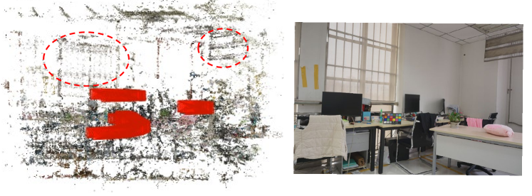
Camera calibration. Since the REVIDE dataset does not provide camera intrinsics, we selected a high-quality continuous indoor video and used COLMAP for 3D reconstruction to obtain the camera intrinsics. The resulting camera trajectory aligns with the movement path of the robotic arm.

Depth-Centric Dehazing and Depth-Estimation from
Real-World Hazy Driving Video

Abstract

Introduction

Related work