Deprojecting Sersic Profiles for Arbitrary Triaxial Shapes: Robust Measures of Intrinsic and Projected Galaxy Sizes
Abstract
We present the analytical framework for converting projected light distributions with a Sérsic profile into three-dimensional light distributions for stellar systems of arbitrary triaxial shape. The main practical result is the definition of a simple yet robust measure of intrinsic galaxy size: the median radius , defined as the radius of a sphere that contains 50% of the total luminosity or mass, that is, the median distance of a star to the galaxy center. We examine how depends on projected size measurements as a function of Sérsic index and intrinsic axis ratios, and demonstrate its relative independence of these parameters. As an application we show that the projected semi-major axis length of the ellipse enclosing 50% of the light is an unbiased proxy for , with small galaxy-to-galaxy scatter of 10% (1), under the condition that the variation in triaxiality within the population is small. For galaxy populations with unknown or a large range in triaxiality an unbiased proxy for is , where is the circularized half-light radius, with galaxy-to-galaxy scatter of 20-30% (1). We also describe how inclinations can be estimated for individual galaxies based on the measured projected shape and prior knowledge of the intrinsic shape distribution of the corresponding galaxy population. We make the numerical implementation of our calculations available.
1. Introduction
The spatial distribution of stars in a galaxy encodes key information about its formation history, whether dissipative or dissipationless processes dominated and whether angular momentum has been retained or lost. The half-light radius is the simplest observational measure of stellar mass distribution. From an empirical perspective, this quantity has played a central role in defining the nature of galaxies through examining and interpreting their scaling relations (e.g., Kormendy, 1977; Djorgovski & Davis, 1987; Dressler et al., 1987) and tracking the build up of galaxies through cosmic time (e.g., Trujillo et al., 2004; van der Wel et al., 2014a). From a theoretical perspective, galaxy sizes have repeatedly revealed that essential physical elements are missing in galaxy formation models (e.g., Navarro & Steinmetz, 2000), leading to the implementation of (astro)physical processes such as feedback.
Measurements of galaxy sizes as traced by stellar light have now reached a point where 0.1 dex accurate statements about two-dimensional (2D) projected galaxy sizes across cosmic time can be made with great precision (e.g., Mowla et al., 2019; van der Wel et al., 2014a). Currently, we are limited by the interpretation of the data, not its scarcity – almost a unicum in the field of galaxy evolution. One limiting factor is the missing link between the projected size (the half-light radius that we measure) and a physically more directly meaningful quantity such as the average or median distance of a star to the center of its galaxy. This conversion factor, from projected to three-dimensinonal (3D) intrinsic size, can vary by large factors given the range of possible galaxy shapes and projections. As a result, comparisons with simulations have remained indirect and prone to systematic effects (e.g., Parsotan et al., 2021; Ludlow et al., 2019; Genel et al., 2018).
We note that we take the word size to mean the 2D projected or 3D intrinsic half-light radius (or, ideally, half-mass radius) that serves to quantify what we define as the mean radius of the galaxy. Other definitions of size adopt a fixed surface brightness or density threshold, aiming to quantify the full extent of the galaxy, which is a useful but qualitatively different quantity from the mean radius.
To our knowledge attempts at the deprojection of measured 2D light profiles so far have assumed spherical symmetry (e,g, Bezanson et al., 2009), symplifying the calculation, but failing to account for the fact that in reality most galaxies are far from spherical: even most early-type galaxies have an intrinsic short-to-long axis ratio of no more than (e.g., Vincent & Ryden, 2005), which more recently has been shown to be the case across cosmic time (e.g., Chang et al., 2013). In this paper we present the analytical framework and numerical implementation for the conversion of 2D light profiles to 3D light distributions for galaxies of arbitrary triaxial shape. Only with this machinery can we take full advantage of the available high-quality data and make accurate comparisons with theoretical predictions.
This papers is organised as follows: Section 2 describes how triaxial shapes project in 2D; Section 3 depicts the deprojection of Sérsic profiles; Section 4 introduces the definition and derivation of the median radius, ; Section 5 outlines how to infer, in practice, from projected size and shape measuremts; Section 6 concludes with a brief description of implications of our findings for galaxy size estimates.
2. Ellipsoidal Shapes
We consider intrinsic density distributions that are constant on ellipsoids
| (1) |
with . The major semi-axis length is a scale parameter, whereas the intermediate-over-major () and minor-over-major () axis ratios determine the intrinsic shape. In the oblate or prolate axisymmetric limit we have (pancake-shaped) or (cigar-shaped), respectively, while in the spherical limit (so then ). Note that is a dimensionless ellipsoidal radius.
We introduce a new Cartesian coordinate system , with and in the plane of the sky and the -axis along the line-of-sight. Choosing the -axis in the -plane of the intrinsic coordinate system (cf. de Zeeuw & Franx, 1989) and their Fig. 2), the transformation between both coordinate systems is known once two viewing angles, the polar angle and azimuthal angle , are specified. The intrinsic -axis projects onto the -axis; for an axisymmetric galaxy model the -axis aligns with the short axis of the projected density,111For an oblate galaxy, the alignment () follows directly from equation (2) since . For a prolate galaxy it is most easily seen by exchanging and (), so that the -axis is again the symmetry axis (instead of the -axis). but for a triaxial galaxy model the -axis is misaligned by an angle such that (cf. equation B9 of Franx, 1988)
| (2) |
where is the triaxiality parameter defined as . A rotation through transforms the coordinate system to such that the and axes are aligned with the major and minor axes of the projected density (respectively), while is along the line-of-sight.
Projecting along the line-of-sight yields a surface density that is constant on ellipses in the sky-plane,
| (3) |
where we have used , and . The sky-plane ellipse is given by
| (4) |
The projected major and minor semi-axis lengths, and , depend on the intrinsic semi-axis lengths , , and and the viewing angles and as follows:
| (5) |
where and are defined as
| (6) | |||||
| (7) | |||||
It follows that is proportional to the area of the ellipse.
The flattening of the projected ellipses actually depends on the viewing angles and the intrinsic axis ratios , and is independent of the scale length. Since the intrinsic and projected semi-major axis lengths are directly related via the left equation of (5), the scale length can be set by choosing either or .
In what follows, we will describe the density and related quantities in terms of mass, including intrinsic mass density, surface mass density and enclosed mass. Without loss of generality, these quantities may also be expressed in terms of light, i.e., intrinsic luminosity density, surface brightness, and enclosed luminosity. However, mixing of mass and light quantities requires an additional conversion with the mass-to-light ratio which in general varies with galactic radius.


3. Deprojected Sérsic density profiles
It has long been known that the stellar surface density profiles of early-type galaxies and of spiral galaxy bulges are well described by a Sersic (1968) profile , with the effective radius enclosing half of the total stellar mass. A key conceptual difference from cusped models is that the profile does not converge to a particular inner slope on small scales. Unfortunately, the deprojection of the Sersic surface density profile cannot be expressed in common functions (for special functions see Baes & van Hese, 2011), but is well approximated by the analytic density profile of Prugniel & Simien (1997)
| (8) |
where the inner negative slope is given by
| (9) |
The enclosed mass for the Prugniel-Simien model is
| (10) |
where is the incomplete gamma function, which in the case of the total luminosity reduces to the complete gamma function .
The expression for the surface density is, to high accuracy, the Sérsic profile
| (11) |
Given the enclosed projected mass
| (12) |
the requirement that the total intrinsic and projected mass have to be equal yields a normalisation
| (13) |
The value of depends on the index and the choice for the scale length. The latter is commonly chosen to be the effective radius in the stellar surface density profile, which contains half of the total stellar mass. We adopt a similar convention requiring that the ellipse contains half of the projected mass. This choice results in the relation , which to high precision can be approximated by (cf. Ciotti & Bertin, 1999)
| (14) |
4. Median radius


We suggest as a robust measure for the size of a galaxy the median spherical radius. To infer this value numerically we have to find the spherical radius which encloses half of the stellar mass. The mass enclosed within a spherical radius follows from
| (15) |
with ellipsoidal radius , where we have defined
| (16) |
and as before and . Substituting the deprojected Sérsic density of equation (8), we see that the integral over radius is an incomplete gamma function, so that
| (17) | |||||
With the total stellar mass given by equation (10) for , the median radius normalized by the scale length , follows upon numerically solving
| (18) | |||||
When in oblate axisymmetry the integral over can be discarded. In case of prolate axisymmetry, it is easiest to exchange and , so that again and the integral over can be discarded, whereas and the resulting has to be divided by to obtain .
As can be seen from Figures 1 and 2, the resulting depends on the intrinsic axis ratios and , but very little on Sérsic index . This implies that the median radius is robust against measurement errors in .
In practice we cannot measure the intrinsic scale length , but instead we measure the projected semi-major axis length and semi-minor axis length . Using the relations (5), we infer the ratio of the median radius to these projected length scales. Figure 3 shows the resulting (solid curves), (dotted curves), and (dashed curves) with the adopted definition , as function of the polar viewing angle .
In the axisymmetric case (top-left panel), the latter polar angle is the inclination , ranging from for edge-on (side-on) to for face-on (end-on) in the oblate (prolate) axisymmetric case, with intrinsic flattening () indicated by the different colors.
In the triaxial case, the polar angle ranges from viewing the short axis from the side () to from the top (). In addition, the projection depends on the azimuthal viewing angle , which ranges from viewing from along the long axis (∘, top-right panel), intermediate between long and short axis (∘, bottom-left panel) to along the intermediate axis (∘, bottom-right panel). The intrinsic short-to-major axis ratio is fixed to , whereas the colors indicate different intrinsic intermediate-to-major axis ratios .
In all four panels the blue curves correspond to the same oblate axisymmetric case , which is independent of the azimuthal angle . Even though the red curves also correspond to the prolate case with the same intrinsic flattening, the orientation in the top-left panel is such that its symmetry long-axis is along the -axis whereas in the remaining panels it is along the -axis. Finally, all curves are for a Sérsic profile with index , but we have seen before that there is little variation with .
5. Applications and Limitations
5.1. Inclination Estimates for Individual Galaxies
For individual galaxies a best-effort inclination estimate makes use of the measured projected axis ratio as well as prior statistical or specific (i.e., from kinematics) knowledge about its intrinsic shape.
We first obtain the probability of viewing the galaxy at angles given its observed ellipticity . Then we combine the intrinsic shape and viewing angle distribution by drawing from and and compute the corresponding distribution of ratios . For this we need to perform a straightforward one-dimensional numerical integral for any given intrinsic (triaxial) shape distribution :
| (19) |
where and
| (20) | |||||
Finally, we combine the distribution in with the observed including measurement uncertainties to derive , or more precisely the distribution .
We note that shape and size are likely correlated, introducing another level of complexity: in that case the assumption adopted by, e.g., Chang et al. (2013) and van der Wel et al. (2014b) of random viewing angles – independent of measured size or axis ratio – no longer holds. Zhang et al. (2019) examine the implications for the reconstruction of the intrinsic shapes of galaxy populations based on projected shape and size distributions (building to a large extent on the work we present now in this paper). They find that for mixed populations of prolate-like and oblate-like systems it is indeed important to do this analysis jointly.
5.2. Size Estimates for Individual Galaxies


A broad application of our work is to determine which (projected) size measurement is the best proxy for the physically meaningful . Traditionally, the circularized effective radius (, in our notation) has been widely used, while others use , the semi-major axis of the ellipse that encloses 50% of the total light. Using our knowledge of the intrinsic shape distribution of galaxies, we demonstrate here the differences between these approaches, and their sensitivity to instrinsic shape variations and viewing angle distributions.
Chang et al. (2013) and van der Wel et al. (2014b) show that most galaxies in the present-day universe have highly-flattened, nearly oblate geometries. Crucially, this shape distribution generally applies to different types of galaxies: star-forming, quiescent, early-type, late-type, with the exception of galaxies of very low and very high mass (see below). We generate two simulated populations of such oblate and near-oblate objects seen at random viewing angles.
First, representing L∗ early-type galaxies (fast rotators), we assume a perfectly oblate population with intrinsic short-to-long axis ratios (Chang et al., 2013), where the error bar reflects the galaxy-to-galaxy Gaussian scatter. The projected size distribution, relative to is shown in Figure 4 (top left). The major axis radius reproduces very closely, regardless of viewing angle, while strongly depends on viewing angle, inducing a large scatter. The median offset is just 18%, but a factor of 2 difference is not a rare occurrence.
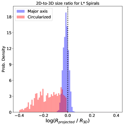
Second, representing L∗ late-type galaxies (spirals), we assume a near-oblate shape distribution with and mild triaxiality to reflect the fact that most spirals are no perfectly circular when viewed face on. Figure 4 (top right) shows similar distributions as for L∗ early-type galaxies, but with a much smaller median value for : . For the early types we see a slight offset from unity for , which is partially due to the lack of any triaxiality and partually due to a higher assumed Sérsic index ( compared to ). The fraction of light projected into a cylinder compared to the light enclosed within a sphere is slightly smaller for high galaxies, but the difference here is just 2%. Of course, for other apertures, e.g., enclosing 20% or 80% of the light these differences are much larger.
It is intuitively obvious that the measured semi-major axis of a disk is invariant with inclination. Therefore, let us consider two classes of galaxies with very different shapes. First, massive elliptical have been shown to be strongly triaxial. According to Chang et al. (2013) massive ellipticals have a triaxility of and intrinsic short-to-long axis ratio of (see also Vincent & Ryden, 2005). For a simulated population of such objects seen at random viewing angles we find medians of and (see Figure 4, bottom left). Perhaps surprisingly, even for massive ellipticals provides a more accurate estimate of than . At the same time, is more precise in the sense that the scatter in is smaller.
Second, high-redshift, low-mass star-forming galaxies, among observed galaxy populations, deviate the most from oblate shapes and therefore provide the most stringest test of our approach. Initiated by the discovery of so-called chain galaxies (Cowie et al., 1995), we have learned that low-mass galaxies at have very diverse geometries, ranging from oblate to prolate (Ravindranath et al., 2006; Yuma et al., 2012; Law et al., 2012; van der Wel et al., 2014b). Adopting and , we find and (see Figure 4, bottom right). Once again, provides a less biased galaxy size, and the scatter is similar for and
| Population | ||||
|---|---|---|---|---|
| L∗ E | 0 | |||
| L∗ S | ||||
| 3L∗ E | ||||
| Irr |
The overall conclusions we draw from this exercise are not as clear-cut as one would like. The decision to use or depends on the situation. If the sample of relevance has a narrow range in triaxiality , then using is preferable because of the lack of bias and small scatter with respect to . The range in oblateness does not affect this decision: the size distribution of a mix of very thick disks (even spheres) and thin disks is still much better described by than . If, on the other hand, the sample spans a wide range of triaxialities – or if the triaxiality is unknown – then using is preferable because of the known, but relatively stable bias. The galaxy-to-galaxy scatter in size is larger in this case, but this is unavoidable in the first place due to the lack of knowledge of the intrinsic shapes.
As a closing remark, let us stress that we explicitly assumed that galaxies are transparent. The effects of viewing-angle dependent extinction is likely the main uncertainty in determining the light-weighted . Furthermore, one would like to measure mass-weighted sizes instead of light-weighted sizes. Mass-to-light ratio gradients due to age and metallicity gradients can have a large effect, with mass-weighted projected sizes that are typically 0.2 dex smaller than light-weighted sizes, to first order independent of galaxy type (e.g., Szomoru et al., 2012; Mosleh et al., 2017; Suess et al., 2019). Ideally, stellar surface mass density maps are used in combination with the methodology developed in this paper to arrive at size estimates that can directly be compared with theoretical models and the results from numerical simulations.
Finally, the numerical implementation of the methods presented here can be made available upon request.
References
- Baes & van Hese (2011) Baes, M., & van Hese, E. 2011, A&A, 534, A69
- Bezanson et al. (2009) Bezanson, R., van Dokkum, P. G., Tal, T., et al. 2009, ApJ, 697, 1290
- Chang et al. (2013) Chang, Y.-Y., van der Wel, A., Rix, H.-W., et al. 2013, ApJ, 773, 149
- Ciotti & Bertin (1999) Ciotti, L., & Bertin, G. 1999, A&A, 352, 447
- Cowie et al. (1995) Cowie, L. L., Hu, E. M., & Songaila, A. 1995, AJ, 110, 1576
- de Zeeuw & Franx (1989) de Zeeuw, T., & Franx, M. 1989, ApJ, 343, 617
- Djorgovski & Davis (1987) Djorgovski, S., & Davis, M. 1987, ApJ, 313, 59
- Dressler et al. (1987) Dressler, A., Lynden-Bell, D., Burstein, D., et al. 1987, ApJ, 313, 42
- Franx (1988) Franx, M. 1988, MNRAS, 231, 285
- Genel et al. (2018) Genel, S., Nelson, D., Pillepich, A., et al. 2018, MNRAS, 474, 3976
- Kormendy (1977) Kormendy, J. 1977, ApJ, 218, 333
- Law et al. (2012) Law, D. R., Steidel, C. C., Shapley, A. E., et al. 2012, ApJ, 745, 85
- Ludlow et al. (2019) Ludlow, A. D., Schaye, J., Schaller, M., & Richings, J. 2019, MNRAS, 488, L123
- Mosleh et al. (2017) Mosleh, M., Tacchella, S., Renzini, A., et al. 2017, ApJ, 837, 2
- Mowla et al. (2019) Mowla, L. A., van Dokkum, P., Brammer, G. B., et al. 2019, ApJ, 880, 57
- Navarro & Steinmetz (2000) Navarro, J. F., & Steinmetz, M. 2000, ApJ, 538, 477
- Parsotan et al. (2021) Parsotan, T., Cochrane, R. K., Hayward, C. C., et al. 2021, MNRAS, 501, 1591
- Prugniel & Simien (1997) Prugniel, P., & Simien, F. 1997, A&A, 321, 111
- Ravindranath et al. (2006) Ravindranath, S., Giavalisco, M., Ferguson, H. C., et al. 2006, ApJ, 652, 963
- Sersic (1968) Sersic, J. L. 1968, Atlas de galaxias australes
- Suess et al. (2019) Suess, K. A., Kriek, M., Price, S. H., & Barro, G. 2019, ApJ, 885, L22
- Szomoru et al. (2012) Szomoru, D., Franx, M., & van Dokkum, P. G. 2012, ApJ, 749, 121
- Trujillo et al. (2004) Trujillo, I., Rudnick, G., Rix, H.-W., et al. 2004, ApJ, 604, 521
- van der Wel et al. (2014a) van der Wel, A., Franx, M., van Dokkum, P. G., et al. 2014a, ApJ, 788, 28
- van der Wel et al. (2014b) van der Wel, A., Chang, Y.-Y., Bell, E. F., et al. 2014b, ApJ, 792, L6
- Vincent & Ryden (2005) Vincent, R. A., & Ryden, B. S. 2005, ApJ, 623, 137
- Yuma et al. (2012) Yuma, S., Ohta, K., & Yabe, K. 2012, ApJ, 761, 19
- Zhang et al. (2019) Zhang, H., Primack, J. R., Faber, S. M., et al. 2019, MNRAS, 484, 5170