Deployment Optimization of Dual-functional UAVs for Integrated Localization and Communication
Abstract
In emergency scenarios, unmanned aerial vehicles (UAVs) can be deployed to assist localization and communication services for ground terminals. In this paper, we propose a new integrated air-ground networking paradigm that uses dual-functional UAVs to assist the ground networks for improving both communication and localization performance. We investigate the optimization problem of deploying the minimal number of UAVs to satisfy the communication and localization requirements of ground users. The problem has several technical difficulties including the cardinality minimization, the non-convexity of localization performance metric regarding UAV location, and the association between user and communication terminal. To tackle the difficulties, we adopt -optimality as the localization performance metric, and derive the geometric characteristics of the feasible UAV hovering regions in 2D and 3D based on accurate approximation values. We solve the simplified 2D projection deployment problem by transforming the problem into a minimum hitting set problem, and propose a low-complexity algorithm to solve it. Through numerical simulations, we compare our proposed algorithm with benchmark methods. The number of UAVs required by the proposed algorithm is close to the optimal solution, while other benchmark methods require much more UAVs to accomplish the same task.
Index Terms:
Wireless localization, integrated localization and communication (ILAC), unmanned aerial vehicle (UAV), geometric deployment.I Introduction
I-A Motivations
Modern 5G communication networks with high speed and low latency are expected to cover most urban areas. New applications enabled by 5G such as remote healthcare, Internet of Vehicles, smart homes, industrial control, and environmental monitoring will bring unprecedented intelligent service experience to citizens [1, 2, 3]. However, urban 5G networks are under the risk of regional service interruption in case of earthquakes, floods or other emergency accidents[4]. Besides, in remote areas such as mountainous environments and wild fields, it is difficult to guarantee smooth communication when performing terrain survey, reconnaissance and rescue operations due to the high deployment cost and insufficient coverage of communications infrastructure. Recently, unmanned aerial vehicle (UAV) technology has emerged as an important solution to assist communication in emergency, where UAV-mounted aerial base stations (BSs) can be flexibly deployed to cover ground users with high-speed and reliable line-of-sight (LoS) communication services[5].
Besides reliable communication services, ground terminals such as rescue devices also demand accurate positioning services in emergency scenarios. The global navigation satellite system (GNSS) can provide satisfactory positioning services in open-sky environments [6]. However, under severe obstructions and scattering in mountainous or disaster environments, the positioning accuracy of GNSS plummets dramatically (e.g., from 5-10 meters root mean square error to tens of meters) and the positioning service suffers from frequent interruptions[7]. Besides, the GNSS has relatively low positioning accuracy in vertical dimension, and thus it cannot provide accurate three-dimensional (3D) localization services required in many emergency scenarios[8]. In addition to GNSS, existing terrestrial cellular networks have independent localization capabilities, where terrestrial BSs can serve as anchor nodes (ANs) to support a variety of localization methods such as observed time difference of arrival (OTDoA) positioning [9]. Achieving high 3D localization accuracy requires not only sufficient number of ANs, but also spatial diversity in the deployment of ANs[10]. For instance, to attain high vertical positioning accuracy, the anchors should differ noticeably in amplitude. When the ground ANs are co-planar, UAVs can be quickly and flexibly deployed as temporary aerial ANs to improve the overall localization accuracy, especially in the vertical dimension. Existing UAV deployment solutions mostly use UAVs for either communication or positioning purpose, and lack efficient coordination with terrestrial networks. As a result, a large number of UAVs are needed to ensure both communication and positioning performance in a large area. In practice, this could lead to large networking delay, high control complexity and signalling overhead.
To minimize the UAV deployment cost of emergency networks, we propose a dual-functional UAV paradigm that utilizes UAVs as both air-based ANs and BSs to provide integrated localization and communication (ILAC) services to ground UEs. Specifically, we consider to deploy multiple dual-functional UAVs working collaboratively with terrestrial BSs to extend the communication and localization service coverage. The key design problem lies in the potential conflicting effects of UAV positions on the communication and localization performance of ground UEs. Intuitively, as an aerial BS, a UAV needs to be deployed close to the ground UEs for stronger communication link quality; as an aerial AN, however, such a close-to-ground UAV deployment may cause large vertical localization error due to its similar altitude with terrestrial anchors. To meet the diverse service requirements of ground UEs, the deployment of UAVs should coordinate with terrestrial BSs to achieve a balanced communication and localization performance.
To this end, this paper aims to answer the following two key questions:
Q1: For a UE at a given target location, how to determine the position of a single dual-functional UAV in an analytical form, such that the UAV and ground BSs can collaboratively satisfy the communication and localization performance requirements of the UE.
Q2: For a set of target UEs distributed over a large area, how to deploy minimum number of dual-functional UAVs within a short computational time, such that the integrated air-ground network can meet the communication and localization performance requirements of all the UEs.
To understand the technical challenges of the above questions, we review in the following some related work using UAVs to provide communication and localization services.
I-B Related Work
I-B1 UAV-assisted Communication
There have been extensive studies in recent years on employing UAVs to assist terrestrial communications. For instance, UAVs are deployed in mobile hot-spots to offload cellular traffic, as aerial relays to tackle obstructions in the ground, as transceivers to collect/disseminate data from/to massive IoT devices in rural areas, and as temporary aerial stations in emergency, etc. UAV deployment is one key design problem in UAV-assisted communications. Depending on the mobility of UAVs, existing studies are mainly divided into two streams: one optimizes the fixed locations of rotary-wing UAVs and the other designs the trajectories of mobile UAVs, including both rotary-wing and fixed-wing UAVs. In this paper, we focus on the former topic to deploy dual-functional UAVs at fixed locations.
Considering a simplified one-dimensional (1D) scenario, the authors in [11] derive the formula of LoS probability between the UAV and the ground users, and optimize the UAV altitude to maximize the UAV communication coverage. For multiple UAVs, the authors in [12] study the optimal altitude of UAVs as relays to minimize the end-to-end outage probability and bit error rate (BER). [13] and [14] further consider the UAV placement for communication in 2D scenario when the UAV altitude is fixed. [13] aims to minimize the number of UAVs to cover a group of ground users by sequentially deploying the UAVs along a spiral path from area perimeter toward the center.[14] jointly optimizes the UAV 2D locations and user transmission power to maximize the user communication rate to both UAVs and multiple terrestrial BSs. Furthermore, recent studies [15, 16, 17] investigate how to deploy UAVs in 3D space to improve the communication performance. Considering using a single UAV as a relay, [15] minimizes the decoding error probability in latency-critical scenarios by optimizing the location and power of the UAV. Using multiple UAVs as relays, [16] searches for the optimal UAV locations to maximize the system communication rate. [17] investigates the problem of determining 3D placement and orientation of the minimal number of UAVs to guarantee the LoS coverage and the signal-to-noise ratio (SNR) between the UAV-UE pairs.
I-B2 UAV-assisted Localization
Besides GNSS, a UE can also estimate its location from the positioning reference signals sent by cellular networks, such as received signal strength (RSS), time of arrival (ToA) and time difference of arrival (TDoA)[18]. Among them, location estimation using TDoA measurements is one popular method used in 4G/5G standard for high-precision localization. The estimation is based on the principle of linear least-square estimation, where at least four ANs are required to obtain an unbiased 3D location estimation. Additional ANs can provide redundancy in the estimation to counter noisy measurements.
Given the deployment of ANs, there have been extensive studies to optimize the resource allocation such as power and bandwidth allocation to minimize the localization error. [19] and [20] study the resource allocation for UAV-assisted vehicle localization using ToA method. Both studies obtain the global optimal solution based on semi-definite programming (SDP) that minimizes the Cramer-Rao lower bound (CRLB) of the localization error. However, minimizing the localization error with respect to UAV anchor deployment is difficult due to the non-convexity of CRLB regarding the UAV position. The current research on UAV deployment and trajectory optimization mainly adopts exploration algorithms, such as genetic algorithms, predetermined-pattern trajectory optimization and particle swarm optimization [21, 22, 23]. [21] plans a static path for a single UAV by selecting a subset of way-points from a predetermined point set to maximize the localization precision. In [22], the authors jointly optimize the UAV positions, power and bandwidth allocation to improve the localization accuracy of vehicles by Taylor expansion-based approximate searching algorithm. Based on RSS measurements, [23] designs the UAV trajectory to assist 3D map estimation using particle swarm optimization. In general, the existing exploration-based methods lack theoretical analysis on the optimal UAV deployment. As a result, the obtained solution often cannot guarantee localization performance and may induce high computational complexity in emergent UAV deployment applications.
I-B3 Summary
To summarize, communication-oriented UAV placement is well-understood from 1D to 3D scenarios. However, localization-oriented UAV placement lacks theoretical characterization and efficient optimization tools. In addition, most work studies the communication and localization problems separately, which may lead to high deployment cost and delay in emergency network. Reusing one UAV for providing both communication and localization services is an effective solution to reduce the network deployment cost, which however is also more challenging considering the potential performance conflict in the dual-functional UAV deployment. To achieve guaranteed quality of service (QoS), we need both theoretical analysis and low-complexity algorithm design for the deployment of dual-functional UAVs.
I-C Contributions
In this paper, we study the optimal deployment problem of dual-functional UAVs that operate collaboratively with ground BSs to provide both communication and localization services to ground UEs. In particular, we are interested in deploying minimal UAVs to satisfy the communication and localization performance requirements of UEs at a set of target locations. Our contributions are summarized as follows.
I-C1 Low-cost networking with dual-functional UAVs
We propose a new integrated air-ground networking paradigm that uses dual-functional UAVs to assist the ground networks for improving both communication and localization services. We consider a UE using OTDoA method to estimate its own location from the positioning signals sent by a UAV and three ground BSs. Besides, each UE communicates to either a UAV or a BS that yields the highest data rate. The proposed dual-functional UAV scheme significantly reduces the cost and delay in the network deployment under emergency.
I-C2 Minimal UAV deployment problem formulation
We formulate a minimal UAV deployment problem that optimizes both the number and locations of UAVs to meet the communication and localization requirements of ground UEs. The problem is very challenging because of the intractable cardinality minimization, the combinatorial UAV-UE communication association, and non-convex UAV location optimization. We solve the problem in two steps. First, we derive the closed-form expression of feasible UAV location to meet the dual performance requirements of each UE. Then, we transform the minimum deployment problem into an equivalent graphical form and design an efficient algorithm accordingly.
I-C3 Geometric characterization of feasible UAV location
We first analyze the feasible deployment location of a UAV that meets the localization accuracy requirement of a UE. Instead of conventional CRLB performance metric, we propose to use D-optimality as the key localization accuracy metric for analytical tractability. We show that, under the D-optimality metric, the feasible location of the UAV can be characterized as a second-order cone in 3D space. Meanwhile, given a fixed altitude, it reduces to an ellipse in 2D projection plane. We derive the closed-form expressions of both the 3D and 2D feasible regions of the UAV.
I-C4 Efficient graphical solution algorithm
With the geometrical characterization of feasible region, we show that the minimal deployment problem can be equivalently transformed to a minimum hitting set problem, which is a classical NP-complete problem that lacks efficient solution. Based on the equivalent graphical formulation, we propose a low-complexity approximate algorithm to tackle the NP-hardness of the problem in large-size emergent networks.
Simulation results show that the proposed method achieves close-to-optimal performance with much lower computational complexity. Besides, compared with conventional scheme with four ground anchors to locate a 3D target, we find that the proposed integrated air-ground network paradigm significantly improves the localization accuracy in both horizontal and vertical directions. This is because the deployed UAV improves not only the altitude diversity, but also the anchor-target localizing link strength especially when the NLoS noise is large in ground-to-ground channels. Overall, the proposed UAV deployment method provides an efficient solution to guarantee both communication and localization performance requirements.
The rest of paper is organized as follows. Section II introduces the system model of UAV-assisted air-ground ILAC scheme and we formulation the minimum UAV deployment problem in Section III. In Section IV and Section V, we analyze the feasible UAV hovering regions and propose a low-complexity deployment algorithm. Section VI presents the simulation results to evaluate the algorithm performance. Lastly, Section VII concludes the paper.
II System Model
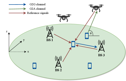
As shown in Fig. 1, we consider an emergency network consisting of 3 terrestrial BSs, rotary-wing UAVs and UEs. The locations of the -th BS, the -th UAV and the -th UE are denoted as , and , respectively.111Notice that the accurate user location is not known and to be estimated. The location is in fact a target user location to receive communication and localization service, e.g., from initial coarse location estimation. A naive way to set the target user locations is dividing the area of interest into equally separated points. Without causing confusions, we use target user location and user location interchangeably in this paper. The UAVs and BSs collaboratively provide communication and localization services to ground UEs.
II-A Communication Model
Considering the occasional blockage between the UAVs and the ground UEs, we adopt the commonly used probabilistic LoS channel model to determine the large-scale attenuation for the ground-to-air (G2A) links[11]. The probability of geometric LoS between the UAV and UE depends on statistical parameters related to the environment and the elevation angle. Specifically, we denote the LoS probability between the UAV at location and UE as , which can be approximated as a modified sigmoid function of the following form [11]
| (1) |
where and are environment-related parameters. is the elevation angle given by
| (2) |
and . Accordingly, the expected channel power gain is equal to
| (3) |
where is the attenuation effect of the NLoS channel, is the path loss exponent and is the reference free space path loss at a distance of 1 m with being the carrier frequency of the G2A channel and being the speed of light. Then, the uplink transmission rate (bits/s) between the user and the UAV is
| (4) |
where is the communication bandwidth, is the transmission power of user , is the noise power spectral density and is the path loss exponent of the G2A channel.
Due to the rich scattering environment in the ground, the ground-to-ground (G2G) channel between the user device and the terrestrial BS can be modeled as a Rayleigh fading channel, which consists of large-scale attenuation and time-varying small-scale fading. We denote the small-scale fading coefficient as and . The instantaneous capacity of the G2G channel is given by
| (5) |
which changes dynamically in the fading channel. Given an outage probability tolerance , an achievable transmission rate (bits/s) of the G2G Rayleigh fading channel can be calculated from Jensen’s inequality as
| (6) |
where is the cumulative distribution function (CDF) of the Rayleigh fading coefficient, which can be obtained from empirical measurements[24]. The power gain of the G2G channel can be derived as
| (7) |
II-B Localization Model
We consider the OTDoA positioning method to localize the ground UEs. To reduce the computational complexity of UE, each UE estimates its 3D location from the reference signals sent by four ANs, including all the three ground BSs and a UAV. We assume that the accurate locations of terrestrial BSs and UAVs are known, since UAVs can use altimeters and satellite systems to locate themselves. Each UE measures the time-of-arrival (ToA) of localization signals from the aerial and terrestrial ANs. The TDoA observations are the time difference between the ToA of a reference node and the ToAs of the remaining ANs. Suppose that all ANs are accurately synchronized in time and BS 1 is the reference node, device estimates its location by solving the TDoA equations:
| (8) |
where is the propagation speed of the signals and is the TDoA between the -th anchor and the reference node BS 1. There exist many linear and non-linear estimation algorithms to obtain from the TDoA equations[25]. In this paper, we are interested in the theoretical bound of localization accuracy regardless of the specific estimation algorithm.
Without loss of generality, we analyze the performance of the OTDoA method by considering the narrowband positioning reference signal (NPRS) in the narrowband IoT (NB-IoT) system. NPRS is an orthogonal frequency division multiplexing (OFDM) based downlink reference signal occupying 180 kHz bandwidth (one LTE resource block). The variance of the ToA measurement using OFDM subframes is expressed as [26]
| (9) |
where and SNR are the symbol duration and signal-to-noise ratio of the received signal, respectively. In one localization period, we have OFDM subframes and each subframe have a set of symbols containing NPRS signal. In symbol , the subset of subcarriers containing NPRS signal is denoted as and is the relative power weight of each subcarrier . According to (9), the variance of the ToA measurement from UAV to UE is given by
| (10) |
where is the NPRS bandwidth, is the noise power density, is the transmission power of the UAV, and is the power gain of G2A channel.
In the G2G channel, advanced signal processing algorithms are needed to eliminate the impacts of multi-path and NLoS propagation on the ToA measurement. The random estimation error is commonly modelled as an additional Gaussian noise term with variance . With the power gain in (7), we derive the variance of the ToA measurements for the G2G channel as
| (11) |
where is the transmission power of the BS . Then, the covariance matrix of the TDoA observations in unit is given by [27]
| (12) |
where var is the variance of variable and cov is the covariance of variables and .
II-C Localization Performance Metrics
The Fisher information matrix (FIM) quantifies the amount of information about the unknown parameter that measurement vector carries. The FIM for OTDoA positioning measurements in (8) is defined as
| (13) |
where is the covariance matrix of OTDoA positioning in unit , and is the Jacobian matrix of the TDoA equations
| (14) |
and the elements in the first and second rows of can be derived as
| (15) |
with . The elements in the third row of can be obtained from (15) by replacing with . There are several localization performance metrics defined based on the FIM. A common metric of localization accuracy is CRLB, which represents the theoretical lower bound of mean square estimation error. CRLB can be expressed as a function of UE location and UAV location , where Tr() means the trace of matrix. However, it is difficult to derive an analytical expression of the feasible UAV location with CRLB. In this paper, we adopt the D-optimality criterion to analyze the localization performance, which is a well-known performance metric of localization accuracy [28]. With the D-optimality metric, we will be able to find intuitive and meaningful geometrical characterizations of UAV deployment in Section IV. Specifically, D-optimality seeks to maximize the following opt- value
| (16) |
The determinant of is inversely proportional to the uncertainty area of an unbiased location estimation [29]. Intuitively, a D-optimality design minimizes the uncertainty ellipsoid, or equivalently, minimize the average location estimation error.
III Problem Formulation
Before formulating the UAV deployment optimization problem, we first provide a motivating example of using UAV to assist the ground localization service. In particular, we show that the proposed UAV-assisted localization method can effectively improve the localization accuracy of the conventional scheme using only terrestrial BSs. For the ease of exposition, we divide an area into small boxes with width of 10 m each. Three BSs are deployed at location , and with unit meter. At each candidate location, we optimize the horizontal placement of the fourth AN at m and calculate the CRLB of the localization variance. For comparison, we place the UAV as the fourth AN at a fixed amplitude 200 m and similarly optimize its horizontal location.222Detailed simulation parameters are provided in the simulation section.
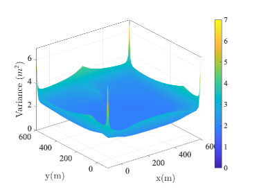
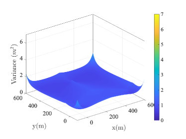
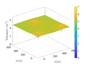
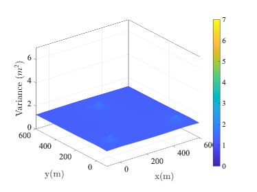
After traversing all the points to be localized, we generate the heap maps in Fig. 2 according to the recorded estimation variance, when is equal to . Each point in the heat map shows the minimum localization variance achievable by optimizing the location of the fourth AN, either the ground BS or UAV. Fig. 2(a) and Fig. 2(b) show the horizontal variance under both designs. Without the UAV, the horizontal variance is in the range of . With UAV as the additional AN, the horizontal variance reduced to the range of . The improvement is more significant in the vertical direction as shown in Fig. 2(c) and Fig. 2(d). The variance ranges are and for the conventional design and the UAV-assisted design, respectively.
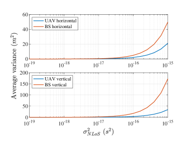
In Fig. 3, we observe the localization accuracy improvement and the conflicting impact of UAV placement. Fig. 3(a) shows the average variance under different NLoS noise. Each sample point is the average performance of 10 localization points distributed in the area with random height from the range m. For both methods, the average variance will increase when the NLoS noise becomes larger. The UAV-assisted localization method produces much lower localization variance than the conventional scheme in both horizontal and vertical directions. The improvement is more significant in the vertical direction when is large. For example, when is equal to , the proposed method reduces horizontal variance and vertical variance. To achieve localization accuracy at 1 m precision in both horizontal and vertical directions, the is required to be lower than for the conventional method and for the UAV-assisted method. The above observations demonstrate the advantage of integrating UAVs for accurate 3D localization, especially in the vertical dimension. That is, the amplitude of UAV AN provides not only strong LoS link quality, but also the critical diversity in AN locations.
With fixed terrestrial BSs, we aim to deploy a minimum number of UAVs to satisfy the localization and communication requirements of all UEs. The problem is formulated as
| (17a) | ||||
| s.t. | (17b) | |||
| (17c) | ||||
| (17d) | ||||
where is the number of UAVs and is the restricted area to deploy the UAVs. Constraint (17b) is the localization accuracy requirement specified by an individual threshold . Constraint (17c) means that the communication rate of UE should be larger than the threshold . The maximization term in (17b) means that each UE estimates its location using all the three ground BSs and only one UAV. Meanwhile, the maximization term in (17c) means that each UE transmits information to only one base station, either a UAV or a ground BS.
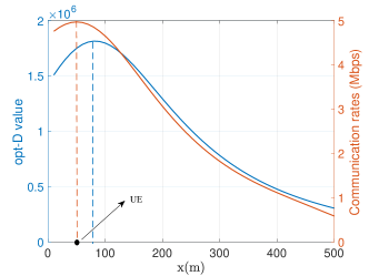
The optimization problem is a cardinality minimization, which is NP-hard in general. An intuitive methodology is to search feasible solutions given fixed cardinality. However, this does not reduce the difficulty because the localization constraints are non-convex in regard to the UAV positions. In addition, contains two implicit association problems between UEs and BSs or UAVs, which are hard combinatorial optimization problems in multi-UAV and multi-BS scenarios. Another major difficulty arises from the potential conflicting impact of UAV placement to the communication and localization performance. As an illustrating example, in Fig. 3(b), we constraint the UAV flying at a fixed amplitude and in a straight line passing over a UE at m. We see that from to m, the communication rate drops while the localization accuracy improves.
Overall, is difficult to solve, and it is even difficult to determine whether there exists a feasible solution satisfying all the constraints given the number of UAVs. In the next section, we analyze the localization performance constraints (17b) and derive closed-form expressions of feasible UAV hovering region.
IV Geometric Characterization of Localization Constraints
In this section, we characterize the localization performance constraint (17b) in a geometric form. This enables the design of efficient graph-based algorithm to solve in the next section.
IV-A Approximation of opt- Value
To facilitate the analysis, we propose in this subsection an approximation of the opt- value for a tagged UE . For simplicity, we drop the index and denote as . We calculate the determinant of the covariance matrix
| (18) |
where . Supposing that , we can ignore the second term and approximate using . Then, we denote the corresponding value as opt-
| (19) |
In contrast, when , we ignore the constant term and approximate using the second term. We denote this approximation as opt-, where
| (20) |
In the following lemma, we show the condition when opt- is an accurate approximation.
Lemma 1.
When , opt- converges to opt-.
Proof:.
The condition implies
| (21) |
Summing up both sides of the three inequalities, we have
| (22) |
which is a sufficient condition for opt- converging to opt-. ∎
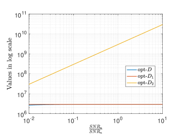
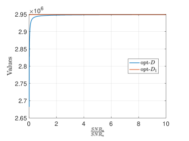
In practice, the random estimation error could be larger than the noise variance of G2A channel , and thus the condition for Lemma 1 is easily satisfied. In Fig. 4(a), we compare the two approximations and the opt- value with different ratios , and depict the values in a log scale. We observe that opt- is much more accurate than opt- within the considered ratio range. In Fig. 4(b), the opt- and opt- values are almost on top with each other when the ratio is greater than 1, and the gap is less that 2% when the ratio is larger than 0.1. Therefore, we can safely adopt opt- as an accurate approximation in the following analysis.
IV-B Equivalent Geometric Characterization
Firstly, we define the unit vector from the -th UAV to a location point as , and that from ground AN to as , where
| (23) | ||||
| (24) |
Then, can be represented by the unit vectors
| (25) |
and we explicitly express using the elements in (15) such that
| (26) |
where the coefficients for are derived using (24)
| (27) | ||||
| (28) | ||||
| (29) |
The localization requirement with opt- approximation in (19) becomes
| (30) |
Based on the value of , we derive the implicit geometry of (30) in two cases.
IV-B1 Case 1
When , constraint (30) is equivalent to
| (31) |
where . The constraint (31) is a standard second-order cone constraint of dimension 4, and it is equivalent to
| (32) |
Geometrically, the relative UAV location that satisfies (32) can be viewed as the intersection of the sphere and the half space . The normal vector of the plane is and the perpendicular distance from the origin to the plane is . The intersecting circle has radius and its center is
| (33) |
For the sphere and plane to have an intersection, it must hold that , i.e., . Accordingly, we establish in the following proposition a condition to check the feasibility of localization requirement.
Proposition 1.
When , the localization requirement for UE at is feasible if and only if the value of satisfies
| (34) |
where and are given by
| (35) |
Proof:.
Please see the detailed proof in Appendix A. ∎
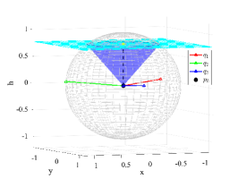
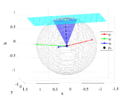
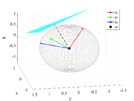
Proposition 1 shows that by setting a reasonably small specified by (34), we can always find a UAV location to satisfy the localization accuracy requirement. Otherwise, if is beyond the range, it could be the case that no UAV placement can achieve the required accuracy level. Fig. 5 showcases that the feasibility of different UE location points under the same settings. For UE location , the localization requirement is feasible when ; for UE location , it is feasible when ; for UE location , it is feasible when . As shown in Fig. 5, under the same , the sphere and the plane has intersection for UE locations and , which means that the localization requirement is feasible for some UAV deployment solution. In Fig. 5(c), the sphere and the plane has no intersection, showing that no UAV deployment can satisfy the localization accuracy requirement for UE location when . Proposition 1 provides a convenient method to set a proper for the constraint (17b) to be feasible. Suppose that all the localization constraints (17b) are feasible by Proposition 1. We continue to derive in the following proposition the feasible UAV hovering region for (17b) assuming the UAV flies at a fixed altitude .
Proposition 2.
For a fixed altitude , the the localization constraint (30) is satisfied if and only if the UAV lies within an ellipse defined by the following polynomial equation
| (36) |
where is the relative altitude. The center of the ellipse, the rotation angle , the semi-major axis and the semi-minor axis are respectively given by
| (37) | ||||
| (38) | ||||
Proof.
We substitute to let the equality in (31) hold. Then, we square both sides of (31) and reformulate it into (2). For an ellipse with the general form
| (39) |
its center , rotation angle , semi-major axis and semi-minor axis are given by
| (40) | |||
| (41) |
By substituting (2) into (39)-(41), we obtain (37) and (38). ∎
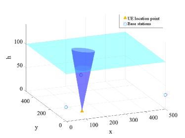
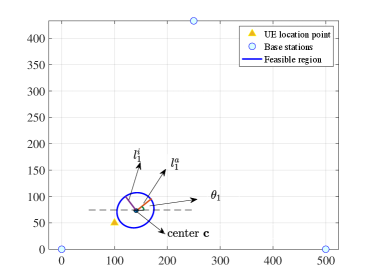
Fig. 6(a) shows the 3D intersection of the extended cone and the plane at m when . Fig. 6(b) shows the 2D projection of the feasible UAV hovering region. We also denote the center, the rotation angle, the semi-major axis and the semi-minor axis of the ellipse in Fig. 6(b). In Fig. 6(a), the UAV must be placed within the cone to satisfy the localization performance constraint. In Fig. 6(b), given a fixed altitude, the UAV must be placed within the eclipse to meet the localization requirement. Although we derive the feasible hovering region for any given in Proposition 2, the distance between UAV and point cannot be too large for two reasons. Firstly, when is too large, the ellipse and its center defined in (2) and (37) could deviate from the UAV restricted area . In this case, we cannot find a feasible UAV location in . Secondly, the strength of localization signal from UAV to UE becomes very weak when the distance is too large, and thus the condition for an accurate opt- approximation no longer holds.
IV-B2 Case 2
When , constraint (30) is equivalent to
| (42) |
where . Similar to the first case, constraint (42) is a standard second-order cone constraint.
Proposition 3.
When , the localization requirement for UE at is feasible if and only if satisfies
| (43) |
where and are the same as in (35).
Proof:.
The proof is similar to that of Proposition 1, and thus we omit it here. ∎
Proposition 4.
For a fixed altitude , the the localization constraint (42) is satisfied if and only if the UAV lies within an ellipse defined by the following polynomial equation
| (44) |
The center of the ellipse, the rotation angle , the semi-major axis and the semi-minor axis are respectively given by
| (45) | ||||
| (46) | ||||
In general, the overall feasible hovering region of a UAV can be specified by the union of two eclipses in Proposition 2 and 4, or just one of them. To simplify the algorithm design to solve in the next section, we prove in the following corollary that we can set a proper value for each UE such that the feasible hovering region of the UAV is specified by only one of the two eclipses in (2) and (4).
Corollary 1.
Proof:.
Please see the detailed proof in Appendix B. ∎
V Proposed Solution
By replacing the opt- value with opt-, we transfer into the following optimization problem
| (47a) | ||||
| s.t. | (47b) | |||
| (47c) | ||||
| (47d) | ||||
In this section, we propose a low-complexity algorithm to solve . In addition to the feasible localization regions specified by Corollary 1, we also need to determine the feasible UAV region to meet communication requirements. According to the communication rate of G2A channel in (4), the communication requirement for UEs is equivalent to
| (48) |
Because is also a function of , it is difficult to depict (48) in graph. To efficiently characterize the feasible region, we restrict the communication requirement by finding a such that it is irrelevant to and satisfies .
Proposition 5.
Let
| (49) |
it holds that .
Proof:.
Please see the detailed proof in Appendix C. ∎
Then, the restricted communication requirement of UE in G2A channels becomes
| (50) |
Notice that (48) is automatically satisfied if (50) holds. Recall that the communication rate of G2G channel is in (6). Then, BS can meet the communication requirement of UE if its location satisfies
| (51) |
Given a fixed altitude , the feasible region of is an ellipse denoted by and the feasible region of the communication requirement is a circle denoted by . We define a region set as , which includes all feasible regions of the communication and localization requirements. Firstly, we consider the communication requirement of each UE. If the location of UE satisfies (51), BS can already serve UE ’s communication demand. We denote the UEs served by BSs as and their corresponding circles as . Then, when considering the placement of UAVs, we can exclude from . Therefore, the new set becomes . Our goal is to select a minimum-size subset of points such that every region in has nonempty intersection with ,. We recognize this as a classical minimum hitting set (MHS) problem, and summarize the solution algorithm to UAV deployment in Algorithm 1.
The MHS problem can be equivalently transferred into an integer liner programming (ILP) problem. The restricted area is first discretized into a set of grid points , which are candidates for the deployment of UAVs. Given the candidate UAV points and the , we use a binary variable to denote that a grid point is in set element , where could be a circle or an ellipse region. Otherwise, we set to be zero. Then, the ILP problem is formulated as
| (52a) | ||||
| s.t. | (52b) | |||
We explain the ILP problem using a simple case with two UEs as shown in Fig. 7. The red circles are the feasible communication regions and the blue ellipses are the feasible localization regions. Therefore, the region set is . The small blue triangles are the candidate points to deploy the UAVs.333The candidate points are randomly selected in space for illustration. In practice, the candidate points could be predetermined or calculated based on environment conditions and parameters. The ILP problem becomes
| (53a) | ||||
| s.t. | (53b) | |||
and the optimal solution is to deploy two UAVs at and . By doing so, all the four circles/eclipses are hit by the two points.
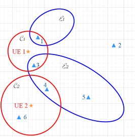
The ILP problem is NP-hard and requires high computational complexity to obtain the optimal solution. Thus, we propose a Depth-first (DF) algorithm to solve the minimum hitting set problem. Firstly, we define the depth of point as , which is equal to the number of regions containing point , i.e., . Then, we select the grid point with the largest depth as the first UAV location. We remove the regions containing and update the depth of grid points. The procedure is repeated until all regions are covered by at least one UAV. We use Fig. 7 to illustrate the algorithm. To start with, we observe that , and have the largest depth 2. Suppose that we firstly select in . Since is in and , we remove these two regions from and update the depth of grid points. Then, we see that has the largest depth as it is inside the regions and . Therefore, we find out that the solution is to deploy UAVs at and . Nonetheless, the proposed solution may lead to suboptimal solution, e.g., selecting in the first step would lead to deploy 3 UAVs at , and . Still, we can improve the performance by executing the algorithm multiple times using randomized selection method and selecting the one produces the best solution.
The computation complexity of Algorithm 2 is , where is the number of grid points and is the number of UEs. The complexity can be further reduced by removing points not in any regions, i.e., , and the number of candidate points would be significantly deducted. The DF algorithm is summarized in Algorithm 2.
VI Simulation Results
| System Parameters | Value | System Parameters | Value |
|---|---|---|---|
| Main frequency, | 2.1 GHz | Free space path loss at 1 m, | 38.89 dB |
| Noise power spectral density, | -174 dbm/Hz | Reference signal bandwidth, | 180 kHz |
| G2A path loss exponent, | 2 | G2G path loss exponent, | 2.2 |
| Transmission power of the BSs, | 1 W | Transmission power of the UAV, | 1 W |
| Transmission power of the UEs, | 0.01 W | UE uplink transmission bandwidth, | 180 kHz |
| Maximum tolerable outage probability | 0.1 | Inverse of the CDF, | 0.11 |
| Environmental parameter, | 15 | Environmental parameter, | 0.5 |
| Symbol duration of the OFDM signal, | s | Number of subframes containing NPRS | 160 |
| Location of BS 1, | Location of BS 2, | ||
| Location of BS 3, |
In this section, we conduct simulation experiments to verify our analysis and evaluate the performance of our proposed algorithm. The simulation parameters are summarized in Table I unless otherwise stated. We compare our proposed algorithm with the following benchmark methods:
VI-1 Integer Linear Programming (ILP) Method
The ILP problem is NP-hard and requires high computational complexity to obtain the optimal solution. We use the solution of ILP method as baseline to evaluate the performance of our proposed method.
VI-2 Communication First Method
In this method, we firstly deploy the UAVs the satisfy the communication requirements of all UEs. The deployed UAVs can satisfy the localization requirements of some UEs. Afterwards, we deploy additional UAVs to meet the localization demands of the remaining UEs.
VI-3 Spiral Searching Method
In [13], the authors proposed a polynomial-time algorithm to sequentially deploy the UAVs along a spiral path toward the center to provide wireless communication coverage to ground users. Similarly, we deploy the UAVs to satisfy the communication and localization requirements of all UEs along a simplified spiral path shown in Fig. 8(a).
VI-4 Strip Searching Method
In [30], the authors proposed a near-linear-time approximation algorithm for the hitting set problem under specific geometric settings. The main idea is to use vertical decomposition to obtain overlapping regions. We adopt the strip searching as a benchmark method, which deploys the UAVs in the sequence shown in Fig. 8(b) from left to right.
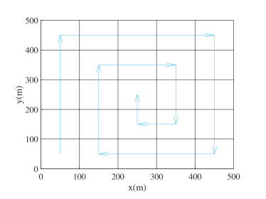
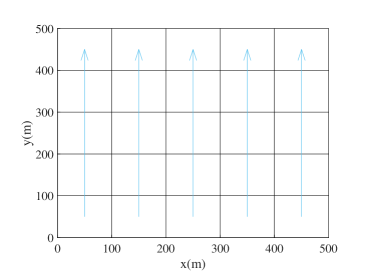
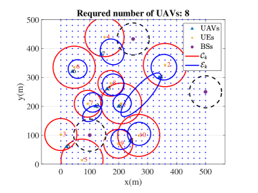
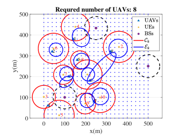
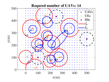
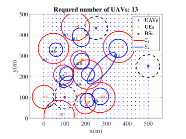
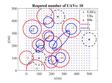
Fig. 9 shows the required numbers and the placements of UAVs under different methods for 10 UEs. The localization accuracy requirement is randomly selected from the range specified by Corollary 1 to ensure feasibility. The communication requirement is randomly chosen from Mbps. Each UE is associated with one circular region (red circle) to meet the communication performance and an elliptical region (blue ellipse) to meet the localization performance. The dashed black circles are the communication coverage of the three BSs. As long as there is a UAV hovering in its corresponding blue area, its localization accuracy requirement is satisfied. Likewise, as long as there is a UAV or ground base station in the red area, the communication requirement can be satisfied. As shown in Fig. 9, the ILP method and the proposed DF method achieve the minimal number of UAVs, which is 8 in this scenario. The spiral searching method and the strip searching method require 13 UAVs and 10 UAVs, respectively. The communication first method requires 14 UAVs, which is the largest among all methods. Although we use the approximation opt- values to determine the feasible localization regions, we find that the obtained UAV locations always satisfy the original localization requirement (17b) in opt- values.
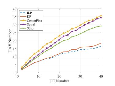
In Fig. 10, we show the average required number of UAVs under all methods from 2 UEs to 40 UEs. Each sample point is the average of 100 simulation runs. The ILP method attains the optimal solutions and provides the baseline for comparison. As shown in Fig. 10, the DF method is the closest to the ILP method. The communication first method and the spiral searching method require more than twice the optimal UAV numbers. The reason is that these methods are based on the communication coverage method. Therefore, they are not suitable for the UAV deployment for joint communication and localization scenarios. The performance of the strip searching method is slightly better than these two methods, which requires less than twice the optimal UAV numbers. When the number of UEs is 40, the average UAV number of the ILP method is . The DF method on average needs more UAVs than the ILP method, while the strip searching method, the spiral searching method and the communication first method require , and more UAVs, respectively.
VII Conclusion
In this paper, we investigate the optimization problem of deploying the minimal number of UAVs in feasible regions to satisfy the communication and localization requirements of the ground users. We compare the localization performance of the UAV-assisted air-ground cooperative ILAC scheme and the conventional scheme using only terrestrial networks. We observe that the scheme with UAVs can greatly improve the localization accuracy in both horizontal and vertical directions. By adopting -optimality as the localization performance metric, we derive the closed-form expression and the spatial characteristics of the feasible UAV hovering regions. We solve the deployment problem by transforming the problem into a geometric minimum hitting set problem, and propose a low-complexity sub-optimal algorithm to solve it. We compare our proposed algorithm with benchmark methods. The number of UAVs required by the proposed algorithm is close to the optimal number, while the other benchmark methods require much more UAVs.
Appendix A Proof of Proposition 1
With and , we have according to Cauchy-Schwartz inequality:
| (54) |
The feasible condition for the intersection of sphere and plane is . Therefore, we have
| (55) |
Since , we have and (55) becomes .
Appendix B Proof of Corollary 1
The general conic equation represents an ellipse if and only if
| (56) |
For (2), condition (56) is equivalent to
| (57) |
Since and we define , the condition is equivalent to
| (58) |
Similarly, because , the condition (56) for (4) is equivalent to
| (59) |
When , in (58) can be discarded. If satisfies , (58) holds while (B) does not hold. When , in (B) can be ignored. If , (B) holds while (58) does not hold.
Appendix C Proof of Proposition 5
Since , we have
| (60) |
In addition, both and are monotonically increasing when , thus implies . Hence, the proof is complete.
References
- [1] C. Hu, W. Fan, E. Zeng, Z. Hang, F. Wang, L. Qi, and M. Z. A. Bhuiyan, “Digital Twin-Assisted Real-Time Traffic Data Prediction Method for 5G-Enabled Internet of Vehicles,” IEEE Transactions on Industrial Informatics, vol. 18, no. 4, pp. 2811–2819, 2021.
- [2] L. Liu, X. Guo, and C. Lee, “Promoting smart cities into the 5G era with multi-field Internet of Things (IoT) applications powered with advanced mechanical energy harvesters,” Nano Energy, vol. 88, p. 106304, 2021.
- [3] M. Kumhar and J. Bhatia, “Emerging communication technologies for 5G-Enabled internet of things applications,” in Blockchain for 5G-Enabled IoT. Springer, 2021, pp. 133–158.
- [4] M. M. Hasan, M. A. Rahman, A. Sedigh, A. U. Khasanah, A. T. Asyhari, H. Tao, and S. A. Bakar, “Search and rescue operation in flooded areas: a survey on emerging sensor networking-enabled IoT-oriented technologies and applications,” Cognitive Systems Research, vol. 67, pp. 104–123, 2021.
- [5] R. Shahzadi, M. Ali, H. Z. Khan, and M. Naeem, “UAV assisted 5G and beyond wireless networks: A survey,” Journal of Network and Computer Applications, vol. 189, p. 103114, 2021.
- [6] X. Zhang, X. Tao, F. Zhu, X. Shi, and F. Wang, “Quality assessment of gnss observations from an android n smartphone and positioning performance analysis using time-differenced filtering approach,” Gps Solutions, vol. 22, no. 3, pp. 1–11, 2018.
- [7] Z. Wang, R. Liu, Q. Liu, L. Han, J. S. Thompson, Y. Lin, and W. Mu, “Toward reliable uav-enabled positioning in mountainous environments: System design and preliminary results,” IEEE Transactions on Reliability, 2021.
- [8] Z. Xiao and Y. Zeng, “An overview on integrated localization and communication towards 6g,” Science China Information Sciences, vol. 65, no. 3, pp. 1–46, 2022.
- [9] S. Fischer, “Observed time difference of arrival (otdoa) positioning in 3gpp lte,” Qualcomm White Pap, vol. 1, no. 1, pp. 1–62, 2014.
- [10] C.-Y. Chen and W.-R. Wu, “Three-dimensional positioning for lte systems,” IEEE Transactions on vehicular technology, vol. 66, no. 4, pp. 3220–3234, 2016.
- [11] A. Al-Hourani, S. Kandeepan, and S. Lardner, “Optimal lap altitude for maximum coverage,” IEEE Wireless Communications Letters, vol. 3, no. 6, pp. 569–572, 2014.
- [12] Y. Chen, W. Feng, and G. Zheng, “Optimum placement of uav as relays,” IEEE Communications Letters, vol. 22, no. 2, pp. 248–251, 2017.
- [13] J. Lyu, Y. Zeng, R. Zhang, and T. J. Lim, “Placement optimization of uav-mounted mobile base stations,” IEEE Communications Letters, vol. 21, no. 3, pp. 604–607, 2016.
- [14] M. A. Ali and A. Jamalipour, “Uav placement and power allocation in uplink and downlink operations of cellular network,” IEEE Transactions on Communications, vol. 68, no. 7, pp. 4383–4393, 2020.
- [15] H. Ren, C. Pan, K. Wang, W. Xu, M. Elkashlan, and A. Nallanathan, “Joint transmit power and placement optimization for urllc-enabled uav relay systems,” IEEE Transactions on vehicular technology, vol. 69, no. 7, pp. 8003–8007, 2020.
- [16] R. Fan, J. Cui, S. Jin, K. Yang, and J. An, “Optimal node placement and resource allocation for uav relaying network,” IEEE Communications Letters, vol. 22, no. 4, pp. 808–811, 2018.
- [17] J. Sabzehali, V. K. Shah, H. S. Dhillon, and J. H. Reed, “3D Placement and Orientation of mmWave-based UAVs for Guaranteed LoS Coverage,” IEEE Wireless Communications Letters, vol. 10, no. 8, pp. 1662–1666, 2021.
- [18] J. A. del Peral-Rosado, R. Raulefs, J. A. López-Salcedo, and G. Seco-Granados, “Survey of Cellular Mobile Radio Localization Methods: From 1G to 5G,” IEEE Communications Surveys & Tutorials, vol. 20, no. 2, pp. 1124–1148, 2018.
- [19] Y. Liu, J. Wang, and Y. Shen, “Spectrum allocation for UAV-aided relative localization of ground vehicles,” in 2018 IEEE International Conference on Communications Workshops (ICC Workshops). IEEE, 2018, pp. 1–5.
- [20] Z. Wu, W. Quan, and T. Zhang, “Resource allocation in UAV-aided vehicle localization frameworks,” in 2019 IEEE/CIC International Conference on Communications Workshops in China (ICCC Workshops). IEEE, 2019, pp. 98–103.
- [21] F. B. Sorbelli, S. K. Das, C. M. Pinotti, and S. Silvestri, “Range based algorithms for precise localization of terrestrial objects using a drone,” Pervasive and Mobile Computing, vol. 48, pp. 20–42, 2018.
- [22] J. Yang, T. Liang, and T. Zhang, “Deployment Optimization in UAV Aided Vehicle Localization,” in 2021 IEEE 93rd Vehicular Technology Conference (VTC2021-Spring). IEEE, 2021, pp. 1–6.
- [23] O. Esrafilian, R. Gangula, and D. Gesbert, “Three-dimensional-map-based trajectory design in UAV-aided wireless localization systems,” IEEE Internet of Things Journal, vol. 8, no. 12, pp. 9894–9904, 2020.
- [24] C. Zhan, Y. Zeng, and R. Zhang, “Energy-efficient data collection in UAV enabled wireless sensor network,” IEEE Wireless Communications Letters, vol. 7, no. 3, pp. 328–331, 2017.
- [25] A. W. Al-Asadi and N. S. Ali, “Noise-Robust Least-Squares Method in TDOA Estimation of a Source Location,” in 2021 Palestinian International Conference on Information and Communication Technology (PICICT), 2021, pp. 123–128.
- [26] J. A. del Peral-Rosado, J. A. López-Salcedo, G. Seco-Granados, F. Zanier, and M. Crisci, “Achievable localization accuracy of the positioning reference signal of 3GPP LTE,” in 2012 International Conference on Localization and GNSS. IEEE, 2012, pp. 1–6.
- [27] Z. Wang, R. Liu, Q. Liu, J. S. Thompson, and M. Kadoch, “Energy-efficient data collection and device positioning in UAV-assisted IoT,” IEEE Internet of Things Journal, vol. 7, no. 2, pp. 1122–1139, 2019.
- [28] D. Ucinski, Optimal measurement methods for distributed parameter system identification. CRC press, 2004.
- [29] Y. Zheng, M. Sheng, J. Liu, and J. Li, “Oparray: Exploiting array orientation for accurate indoor localization,” IEEE Transactions on Communications, vol. 67, no. 1, pp. 847–858, 2018.
- [30] P. K. Agarwal, E. Ezra, and M. Sharir, “Near-linear approximation algorithms for geometric hitting sets,” Algorithmica, vol. 63, no. 1, pp. 1–25, 2012.