Density Regression and Uncertainty Quantification with Bayesian Deep Noise Neural Networks

Daiwei Zhang
Department of Biostatistics
University of Pennsylvania
Philadelphia, PA 19104
[email protected]
&Tianci Liu
School of Electrical and Computer Engineering
Purdue University
West Lafayette, IN 47907
[email protected]
&Jian Kang
Department of Biostatistics
University of Michigan
Ann Arbor, MI 48105
[email protected] Corresponding author

Abstract

Deep neural network (DNN) models have achieved state-of-the-art predictive accuracy in a wide range of supervised learning applications. However, accurately quantifying the uncertainty in DNN predictions remains a challenging task. For continuous outcome variables, an even more difficult problem is to estimate the predictive density function, which not only provides a natural quantification of the predictive uncertainty, but also fully captures the random variation in the outcome. In this work, we propose the Bayesian Deep Noise Neural Network (B-DeepNoise), which generalizes standard Bayesian DNNs by extending the random noise variable from the output layer to all hidden layers. The latent random noise equips B-DeepNoise with the flexibility to approximate highly complex predictive distributions and accurately quantify predictive uncertainty. For posterior computation, the unique structure of B-DeepNoise leads to a closed-form Gibbs sampling algorithm that iteratively simulates from the posterior full conditional distributions of the model parameters, circumventing computationally intensive Metropolis-Hastings methods. A theoretical analysis of B-DeepNoise establishes a recursive representation of the predictive distribution and decomposes the predictive variance with respect to the latent parameters. We evaluate B-DeepNoise against existing methods on benchmark regression datasets, demonstrating its superior performance in terms of prediction accuracy, uncertainty quantification accuracy, and uncertainty quantification efficiency. To illustrate our method’s usefulness in scientific studies, we apply B-DeepNoise to predict general intelligence from neuroimaging features in the Adolescent Brain Cognitive Development (ABCD) project.

1 Introduction

Deep neural networks (DNNs) [1, 2] have achieved outstanding prediction performance in a wide range of artificial intelligence (AI) applications [3, 4, 5, 6, 7, 8, 9, 10]. Despite overwhelming cases of success, a major drawback of standard DNNs is the lack of reliable uncertainty quantification (UQ) [11]. UQ is an essential task in safety-critical AI applications [12]. For example, in medical diagnosis, an individualized risk assessment AI model should be able to report its confidence in its predictions. When the AI model is not sufficiently certain in its assessment of a patient, the patient should be referred to human physicians for further evaluation [13, 14].

In this work, we seek to solve the problem of UQ in DNN regression tasks. In a standard DNN regression model, the outcome $y_{i}$ and the predictors $\bm{x}_{i}$ are assumed to follow the relation $y_{i}=f(\bm{x}_{i})+\epsilon_{i}$ , where the mean function $f(\bm{x}_{i})=\mathrm{E}(y_{i}\mid\bm{x}_{i})$ is constructed by a DNN, and the random noise $\epsilon_{i}$ follows a zero-mean homoscedastic Gaussian distribution $\epsilon_{i}\overset{\text{iid}}{\sim}\mathcal{N}(0,\sigma^{2})$ for some unknown $\sigma^{2}>0$ . This formulation implies the conditional variance of the outcome variable $\operatorname{Var}(y_{i}\mid\bm{x}_{i})$ , given the predictor, to be constant. However, in real applications, the true conditional distribution could be heteroscedastic Gaussian (i.e. $\operatorname{Var}(y_{i}\mid\bm{x}_{i})=\sigma^{2}(\bm{x}_{i})$ ) or not Gaussian at all (e.g. the distribution of $\epsilon_{i}$ is asymmetric or multimodal). In these cases, common UQ statistics derived from Gaussian models (e.g. predictive variance) may fail to capture important patterns in the data, causing UQ to be misleading or inefficient. Therefore, in order to achieve accurate UQ in DNN regression problems, it is critical to learn the conditional density of the outcome variable given the predictors, since the conditional density not only fully quantifies prediction uncertainty, but also gives a complete picture of possible variation in the outcome. We refer to the problem of estimating the conditional density function given the predictors as the density regression (DR) problem, following the terminology in [15]. In this work, we focus on DR tasks with DNNs and treat UQ as a byproduct of DR.

1.1 Related Work

To estimate the conditional density of the outcome given the predictors, many DNN-based frequentist DR methods have been proposed [16, 17, 18, 19]. A conceptually straightforward DR method is to extend the conditional distribution of the outcome from Gaussian to Gaussian mixture, such as in mixture density networks [20, 21] and deep ensembles [22]. An alternative approach is to estimate the prediction intervals without distribution assumptions on the outcome [23, 24], which is closely related to quantile-based models [25, 26]. Other solutions include converting the continuous outcome into a multi-class categorical variable by using bins [27] and estimating the cumulative distribution function (CDF) directly [28].

Compared to ad hoc frequentist UQ and DR methods, the Bayesian framework for DNNs, or Bayesian neural networks (BNNs) [29, 30, 31], provides a more natural and systematic way to model uncertainty in the outcome, i.e. by using the posterior predictive distribution. Theoretically, the posterior prediction intervals are well-calibrated asymptotically [32, 33, 34]. In addition to the capacity of UQ, the Bayesian framework improves the prediction accuracy of deterministic DNNs [35, 36]. Regardless of the aptness of BNNs for UQ, due to the intractability of their posterior distributions, one must resort to variational inference (VI) or Markov Chain Monte Carlo (MCMC) simulation for posterior computation. VI methods [37, 38, 39] approximate the posterior distribution with simpler distributions [40, 41, 42, 43, 44]. Common randomness-based regularization techniques for deterministic DNNs, such as dropout [45, 46, 47], batch normalization [48, 49], and random weights [50, 51], can be interpreted as special cases of VI. However, although computationally efficient, VI methods induce extra approximation errors in learning the posterior distribution, with the parameter variance and covariance often underestimated or oversimplified [37].

In contrast, MCMC methods simulate the exact posterior distribution of the BNN. The most popular MCMC algorithm for modern applications is arguably the Metropolis-Hastings (MH) algorithm [52, 53, 54]. However, even with the assistance of efficient techniques such as Hamiltonian dynamics [55, 56], Langevin dynamics [57], stochastic gradients [58, 59], and mini-batches [60], the ultrahigh dimensionality of BNNs has caused prohibitive computation cost for MH algorithms [61, 62]. An alternative MCMC simulation method is Gibbs sampling [63, 64, 65], where each model parameter (or a block of parameters) is sampled from the conditional posterior distribution given all the other parameters. Although block-wise Gibbs sampling solves the so-called curse of dimensionality for models with a high number of parameters [66], its applications to standard BNNs are impractical if not impossible, due to the lack of closed-form full conditional posterior distributions in standard BNNs with nonlinear activation functions. Finally, most existing BNN methods (including both MCMC- and VI-based) focus on UQ, whereas the problem of DR with DNN is scarcely studied in the Bayesian framework [15].

For UQ and DR with DNN, a related topic is the incorporation of latent noise in the hidden layers. However, existing works on latent noise in DNNs primarily use it as a means for regularization [67, 68]. The potential of stochastic activation layers for UQ was briefly discussed in [69], but the context of this work was classification tasks, where the predictive uncertainty could already be fully characterized by well-calibrated categorical distributions without using any latent noise. More recently, [70] formulated DNNs as latent variable models and included kernel maps in the input layer to avoid feature collinearity. Although the proposed model was capable of UQ, the more challenging problem of DR was not studied.

1.2 Our Contributions

To address the existing issues associated with DR and UQ for DNNs, we propose the Bayesian Deep Noise Neural Network (B-DeepNoise). B-DeepNoise generalizes standard BNNs by adding latent random noise both before and after every activation layer. Although the latent random noise variables independently follow Gaussian distributions, their composition across multiple layers with non-linear activations can generate highly complex predictive density functions. Moreover, the unique structure of B-DeepNoise induces closed-form full conditional posterior distributions for the model parameters, which eliminates the primary barrier for Gibbs sampling in DNN-based models and therefore makes it possible to simulate the exact posterior distribution without using computationally intensive MH algorithms.

To our best knowledge, this is the first work on estimating complex predictive density functions by utilizing DNNs with latent random noise. Furthermore, no previous work has developed Gibbs sampling algorithms for DNN-based Bayesian models. In short, our work contributes to the existing literature on DR and UQ with DNNs in the following ways:

•

We propose a Bayesian DNN model that is capable of learning a wide range of complex (e.g. heteroscedastic, asymmetric, multimodal) predictive density functions.
•

We develop a Gibbs sampling algorithm for the posterior computation of our model that can be implemented by using common samplers and without the need of MH steps.
•

We perform theoretical analysis of our method and obtain analytic expressions of the predictive density and variance propagation.
•

We compare our model with existing methods on synthetic and real benchmark datasets and demonstrate its usefulness in a neuroimaging study.

2 Model Description

2.1 DNNs with latent noise variables

Suppose the data consist of $N$ observations. For $n=1,\ldots,N$ , let $\bm{x}^{(n)}\in\mathbb{R}^{P}$ be the predictors and $\bm{y}^{(n)}\in\mathbb{R}^{Q}$ be the outcome variable. Let $\mathcal{N}(\bm{\mu},\bm{\Sigma})$ be a Gaussian distribution with mean $\bm{\mu}$ and covariance $\bm{\Sigma}$ . To specify the nonlinear association between $\bm{y}^{(n)}$ and $\bm{x}^{(n)}$ , a standard $L$ -layer feed-forward DNN model with Gaussian noises can be represented as

		$\displaystyle[\bm{y}^{(n)}\mid\bm{u}_{L}^{(n)}]\overset{\text{iid}}{\sim}\mathcal{N}\left(\bm{\beta}_{L}\bm{u}^{(n)}_{L}+\bm{\gamma}_{L},\bm{T}_{L}\right),\qquad\bm{u}^{(n)}_{0}=\bm{x}^{(n)},$		(1)
		$\displaystyle\bm{u}^{(n)}_{l+1}=h\Big{(}\bm{\beta}_{l}\bm{u}^{(n)}_{l}+\bm{\gamma}_{l}\Big{)},\qquad l\in\{1,\ldots,L-1\}$		(2)

where $\bm{\beta}_{l}\in\mathbb{R}^{{K_{l}}\times K_{l-1}}$ and $\bm{\gamma}_{l}\in\mathbb{R}^{K_{l}}$ are unknown parameters, $K_{l}$ is the number of units in the $l$ th layer, and $h(\cdot)$ is an element-wise nonlinear activation function, such as the rectified linear unit (ReLU) function and logistic function. In this formulation, $\bm{u}^{(n)}_{L}$ is a deterministic function of $\bm{x}^{(n)}$ . This implies that $\bm{y}^{(n)}$ given $\bm{x}^{(n)}$ follows the same conditional distribution as $\bm{y}^{(n)}$ given $\bm{u}_{L}^{(n)}$ , i.e., a homoscedastic Gaussian distribution with constant covariance $\bm{T}_{L}$ . To model more complex conditional distribution, we propose the Deep Noise Neural Network (DeepNoise), which generalizes Equation 2 of the standard DNN model by including noise variables before and after every activation layer: for $l\in\{1,\ldots,L-1\}$ ,

\displaystyle\bm{u}^{(n)}_{l+1}=h\Big{(}\bm{\beta}_{l}\bm{u}^{(n)}_{l}+\bm{\gamma}_{l}+\bm{\epsilon}^{(n)}_{l}\Big{)}+\bm{\delta}^{(n)}_{l},\qquad\bm{\epsilon}^{(n)}_{l}\overset{\text{iid}}{\sim}\mathcal{N}\Big{(}\bm{0},\;\bm{T}_{l}\Big{)},\qquad\bm{\delta}^{(n)}_{l}\overset{\text{iid}}{\sim}\mathcal{N}\Big{(}\bm{0},\ \bm{\Sigma}_{l}\Big{)},

(3)

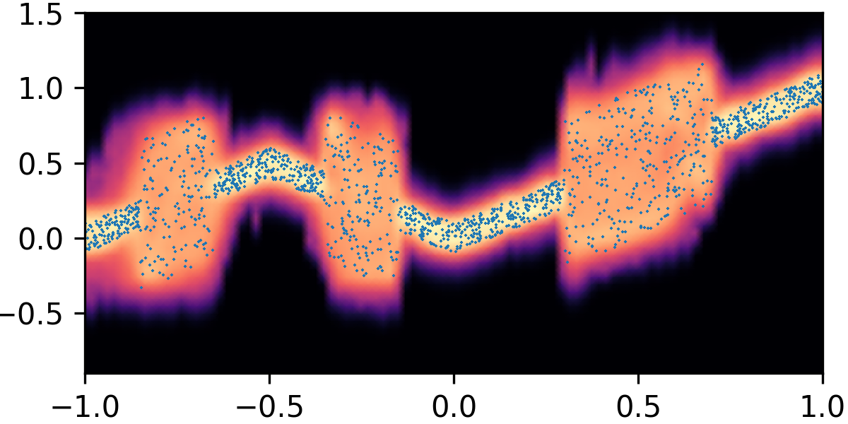
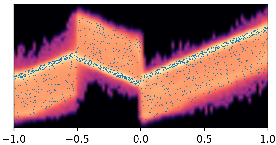
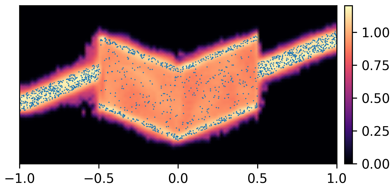
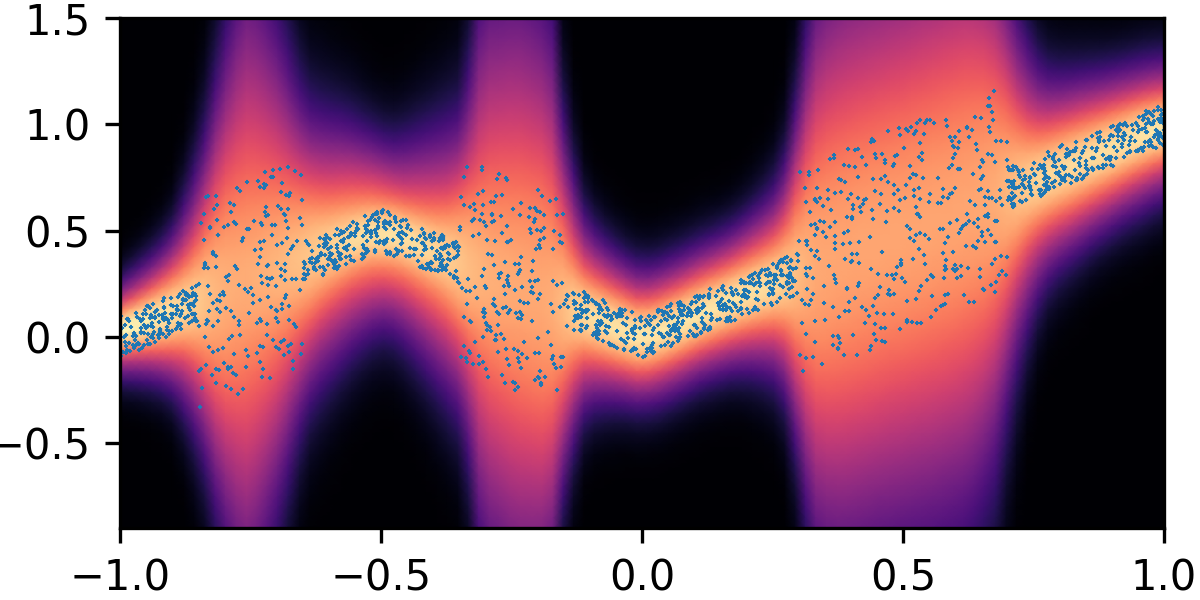
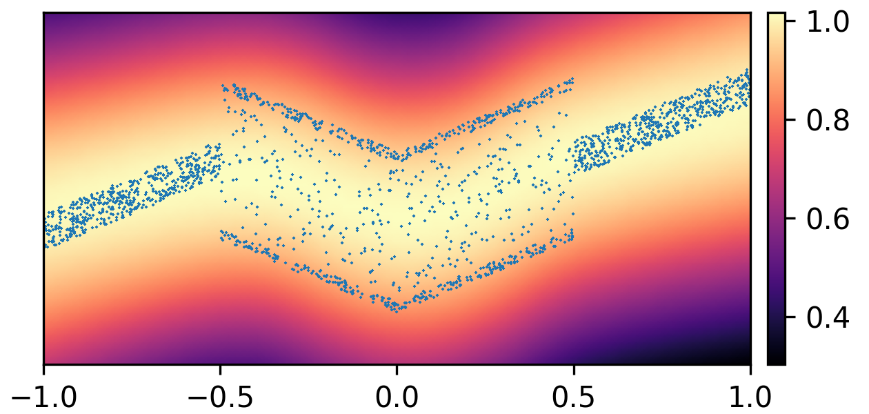
where $\bm{T}_{l}=\operatorname{diag}\{\bm{\tau}^{2}_{l}\}$ and $\bm{\Sigma}_{l}=\operatorname{diag}\{\bm{\sigma}^{2}_{l}\}$ with $\bm{\tau}^{2}=(\tau^{2}_{l,1},\ldots,\tau^{2}_{l,K_{l}})^{\top}$ and $\bm{\sigma}^{2}_{l}=(\sigma^{2}_{l,1},\ldots,\sigma^{2}_{l,K_{l}})^{\top}$ . By composing the latent Gaussian noise variables with linear maps and non-linear activations, DeepNoise is capable of representing a wide range of heteroscedastic Gaussian and non-Gaussian conditional density functions (e.g. asymmetric, multimodal), as illustrated in Figure 1. Intuitively, as Gaussian mixtures are universal approximators of densities ([71], [72], [1, Sec. 3.9.6]) and DNNs are universal approximators of functions [73, 74, 75], DeepNoise is designed to be a universal approximator of conditional densities. The nonparametric nature of DeepNoise enables it to approximate increasingly complex conditional density functions by increasing the number of hidden layers and the number of nodes per layer.

Refer to caption — Figure 1: Observed data (blue dots) and estimated predictive density (heatmap) by B-DeepNoise (top row), DE (middle row), and VI (bottom row) for heteroscedastic (left column), asymmetric (middle column), and multimodal (right column) noise.

2.2 Model Representation and Prior Specifications

DeepNoise transforms the predictor vector into the outcome vector by iteratively applying the linear-noise-nonlinear-noise maps. Thus, the DeepNoise model defined by combining Equations 1 and 3 is equivalent to:

	$\displaystyle\Big{[}\bm{v}_{l}^{(n)}\mid\bm{u}^{(n)}_{l}\Big{]}\;\overset{\text{iid}}{\sim}\;\mathcal{N}$	$\displaystyle\bigg{(}\bm{\beta}_{l}\bm{u}^{(n)}_{l}+\bm{\gamma}_{l},\;\bm{T}_{l}\bigg{)},$	$\displaystyle\text{for }l=0,\ldots,L$		(4)
	$\displaystyle\Big{[}\bm{u}^{(n)}_{l+1}\mid\bm{v}_{l}^{(n)}\Big{]}\;\overset{\text{iid}}{\sim}\;\mathcal{N}$	$\displaystyle\bigg{(}h\Big{(}\bm{v}^{(n)}_{l}\Big{)},\;\bm{\Sigma}_{l}\bigg{)},$	$\displaystyle\text{for }l=0,\ldots,L-1$		(5)

where $\bm{u}^{(n)}_{0}=\bm{x}^{(n)}$ and $\bm{v}^{(n)}_{L}=\bm{y}^{(n)}$ . Write $\bm{\beta}_{l}=(\beta_{l,k,k^{\prime}})$ and $\bm{\gamma}_{l}=(\gamma_{l,k})$ . To make fully Bayesian inference, we impose normal-inverse-gamma prior distributions on the weight-bias parameters:

\displaystyle\beta_{l,k,k^{\prime}}\overset{\text{iid}}{\sim}\mathcal{N}(0,\rho_{l,k,k^{\prime}}^{2}),\quad\gamma_{l,k}\overset{\text{iid}}{\sim}\mathcal{N}(0,\xi_{l,k}^{2}),\quad\rho_{l,k,k^{\prime}}^{2}\overset{\text{iid}}{\sim}\mathcal{IG}(a_{\text{weight}},b_{\text{weight}}),\quad\xi_{l,k}^{2}\overset{\text{iid}}{\sim}\mathcal{IG}(a_{\text{bias}},b_{\text{bias}})

and assign inverse-gamma prior distributions to the pre-activation and post-activation noise variances:

\displaystyle\tau_{l,k}^{2}\overset{\text{iid}}{\sim}\mathcal{IG}(a_{\text{preact}},b_{\text{preact}}),\qquad\sigma_{l,k}^{2}\overset{\text{iid}}{\sim}\mathcal{IG}(a_{\text{postact}},b_{\text{postact}}).

We refer to (4) and (5) along with the prior specifications above as the Bayesian Deep Noise Neural Network (B-DeepNoise) model. Although DeepNoise (i.e. Equations 4 and 5 without the prior distributions) is an effective frequentist model, for the rest of the paper, we focus on B-DeepNoise and conduct theoretical, computational, and empirical analyses in the Bayesian framework.

2.3 Posterior Computation

Compared to standard DNNs and BNNs, the addition of latent random noises not only provides B-DeepNoise with more flexibility for approximating complex predictive density functions, but also provides closed-form expressions of the full conditional posterior distributions of the model parameters. The latter advantage makes it possible to derive efficient Gibbs sampling algorithms for B-DeepNoise. The model parameters are naturally grouped into five categories: pre-activation random noises $\bm{v}^{(n)}_{l}$ , post-activation random noises $\bm{u}^{(n)}_{l}$ , weights and biases $\bm{\beta}_{l},\bm{\gamma}_{l}$ , weight and bias variances $\bm{\rho}^{2}_{l},\bm{\xi}^{2}_{l}$ , and random noise variances $\bm{\tau}^{2}_{l},\bm{\sigma}^{2}_{l}$ . We derive the full conditional posterior distributions for each of these groups of parameters.

The most complex parameter group is the pre-activation random noises $\bm{v}^{(n)}_{l}$ , since their full conditional posterior distributions involves the nonlinear activation function. To develop straightforward Gibbs samplers, we require the activation function to be piecewise linear, as defined in 1.

Assumption 1.

The activation function can be expressed as $h(t)=\sum_{j=1}^{J}(b_{j}t+b^{\prime}_{j})\cdot\mathbb{I}\{t\in[c_{j-1},c_{j})\}$ for some $J\in\mathbb{N}_{+}$ , $b_{1},\ldots,b_{J},b^{\prime}_{1},\ldots,b^{\prime}_{J}\in\mathbb{R}$ , and $-\infty=c_{0}<c_{1}<\ldots<c_{J-1}<c_{J}=\infty$ .

Remark.

The family of functions defined in 1 includes many common activation functions, such as ReLU and leaky ReLU [76]. Moreover, smooth activation functions can be approximated by piecewise linear functions. For example, the logistic, tanh, and softplus functions can be approximated by the hard sigmoid, hard tanh, and ReLU functions, respectively.

We now derive the full conditional posterior distributions of the pre-activation latent noise. Let $\mathcal{TN}(\lambda,\omega^{2},c_{a},c_{b})$ be a truncated normal distribution on interval $[c_{a},c_{b}]$ with location $\lambda$ and scale $\omega$ . Let $\phi_{\mathcal{N}}(\cdot\mid\mu,\sigma^{2})$ be the PDF of the normal distribution with mean $\mu$ and variance $\sigma^{2}$ . Let $\Phi_{\mathcal{N}}(\cdot)$ be the CDF of the standard normal distribution.

Theorem 1.

Suppose the activation function $h$ satisfies 1. For $n\in\{1,\ldots,N\}$ , $l\in\{0,\ldots,L\}$ , and $k\in\{1,\ldots,K_{l}\}$ , let $\omega_{n,l,k,j}^{2}=\Big{(}\tau_{l,k}^{-2}+\sigma_{l,k}^{-2}b_{j}^{2}\Big{)}^{-1}$ and
$\lambda_{n,l,k,j}=\tau_{l,k}^{-2}\omega_{n,l,k,j}^{2}\Big{(}\gamma_{l,k}+\bm{\beta}_{l}\bm{u}_{l}^{(n)}\Big{)}+\sigma_{l,k}^{-2}b_{j}\omega_{n,l,k,j}^{2}\Big{(}u^{(n)}_{l+1,k}-b^{\prime}_{j}\Big{)}$ .
Define $\zeta_{n,l,k,1}=1$ , $\zeta_{n,l,k,j}=\zeta_{n,l,k,j-1}\zeta^{\prime}_{n,l,k,j}$ , where $\zeta^{\prime}_{n,l,k,j}=\kappa_{j,j-1}\kappa_{j-1,j-1}^{-1}\tilde{\kappa}_{j-1,j-1}\tilde{\kappa}_{j,j-1}^{-1}$ with $\kappa_{j,j^{\prime}}=\phi_{\mathcal{N}}(u^{(n)}_{l+1,k}\mid c_{j^{\prime}}b_{j}+b^{\prime}_{j},\sigma_{l,k}^{2})$ and $\tilde{\kappa}_{j,j^{\prime}}=\phi_{\mathcal{N}}(c_{j^{\prime}}\mid\lambda_{n,l,k,j},\omega_{n,l,k,j}^{2})$ . Moreover, let $c^{\prime}_{j,j^{\prime}}=(c_{j^{\prime}}-\lambda_{n,l,k,j})\omega_{n,l,k,j}^{-1}$ , $\pi^{\prime}_{n,l,k,j}=\Phi_{\mathcal{N}}(c^{\prime}_{j,j})-\Phi_{\mathcal{N}}(c^{\prime}_{j,j-1})$ and $\pi_{n,l,k,j}\propto\pi^{\prime}_{n,l,k,j}\zeta_{n,l,k,j}$ . The conditional posterior distribution of pre-activation noise $v^{(n)}_{l,k}$ given the rest of the parameters is

\displaystyle\Big{[}v_{l,k}^{(n)}\Bigm{|}\mathrm{rest}\Big{]}\sim

\displaystyle\sum_{j=1}^{J}\pi_{n,l,k,j}\cdot\mathcal{TN}\Big{(}\lambda_{n,l,k,j},\;\omega_{n,l,k,j}^{2},\;c_{j-1},\;c_{j}\Big{)}.

(6)

Remark.

Intuitively, the piecewise linear property of the activation function causes the full conditional posterior distribution of $\bm{v}^{(n)}_{l}$ to be “piecewise normal”, i.e. a mixture of truncated normal distributions with adjacent truncation endpoints. By using Theorem 1, $\bm{v}^{(n)}_{l}$ can be easily simulated by using samplers for categorical distributions and truncated normal distributions, which are widely available in scientific computation software. In addition, the number of mixing components, which depends on the activation function, is usually very small (e.g. 2 for ReLU and 3 for hard tanh).

The full conditional posterior distributions of the rest of the model parameters are either normal or inverse-gamma, because of the conjugate priors, as shown in Proposition 5 in Appendix A. The derivations are similar to those for Bayesian linear regression with conjugate priors [21, Sec. 2.3.3]. The complete algorithm is described in Algorithm 1 in Appendix A. Note that the predictive distribution only depends on the weight-bias parameters and the latent noise variance parameters. To speed up the computation, these parameters can be initialized by gradient-based optimization algorithms. In addition, the sampling steps in Algorithm 1 can be parallelized across layers and across training samples, making it possible to sample the latent random noises by mini-batches.

2.4 Predictive Density

We further evaluate the properties of the predictive density function. Theorem 2 expresses the predictive density in a recursive formulation. Let $\phi_{\mathcal{MVN}}(\cdot;\bm{\mu},\bm{\Sigma})$ be a multivariate normal density function with mean $\bm{\mu}$ and covariance $\bm{\Sigma}$ .

Theorem 2.

For $l\in\{0,\ldots,L\}$ , let $\bm{\theta}_{l}=\{\bm{\beta}_{l},\bm{\gamma}_{l},\bm{T}_{l},\bm{\Sigma}_{l}\}$ and $\bm{\Theta}_{l}=\{\bm{\theta}_{l^{\prime}}\}_{l^{\prime}=0}^{l}$ . In a B-DeepNoise model, the conditional density of the output $\bm{y}=\bm{v}_{L}$ given input value $\bm{x}$ and model parameters $\bm{\Theta}_{l}$ can be iteratively constructed by

\displaystyle f(\bm{v}_{l}\mid\bm{x},\bm{\Theta}_{l})=

\displaystyle\int_{\mathbb{R}^{K_{l-1}}}\phi_{\mathcal{MVN}}\Big{\{}\bm{v}_{{l}}\Bigm{|}\bm{\gamma}_{l}+\bm{\beta}_{l}h(\bm{v}_{l-1}),\bm{T}_{l}+\bm{\beta}_{l}\bm{\Sigma}_{l}\bm{\beta}_{l}^{\top}\Big{\}}f(\bm{v}_{l-1}\mid\bm{x},\bm{\Theta}_{l-1})d\bm{v}_{l-1},

for $l\in\{1,\ldots,L\}$ and $f(\bm{v}_{0}\mid\bm{x},\bm{\theta}_{0})=\phi_{\mathcal{MVN}}(\bm{v}_{0}\mid\bm{\gamma}_{0}+\bm{\beta}_{0}\bm{x},\bm{T}_{0})$ .

Remark.

As shown in Theorem 2, the predictive distribution given an input value can be expressed as a continuous mixture of multivariate normal (CMMVN) distributions, where the mixing density is another CMMVN, depending on the intermediate values of the previous layer. Although this highly flexible predictive density does not have a closed-form expression, it can be simulated easily by adding normal noise to the intermediate values of the hidden layers, as stated in Equations 4 and 5.

In standard DNNs and BNNs, predictive variance is completely determined by the variance of the noise variable in the last layer. As a more general model, B-DeepNoise propagates variations in the latent random noises to produce complex variation in the outcome. When the variances of the latent random noises are all zero, B-DeepNoise is reduced to a standard BNN. A natural question is how the variance in the output variable can be decomposed into variance of the latent random noises. Theorem 3 bounds the outcome variance by the other model parameters.

Theorem 3.

Let $\bm{y}$ be the output value of the B-DeepNoise model given input value $\bm{x}$ and model parameters $\bm{\Theta}=\{\bm{\beta}_{l},\bm{\gamma}_{l},\bm{T}_{l},\bm{\Sigma}_{l}\}_{l=0}^{L}$ . Let $g(\bm{x},\bm{\Gamma})$ be the output value of the standard DNN model with the same activation function and weight-bias parameters $\bm{\Gamma}=\{\bm{\beta}_{l},\bm{\gamma}_{l}\}_{l=0}^{L}$ . (Note that $\bm{y}$ equals to $g(\bm{x},\bm{\Gamma})$ with probability one when all the latent noise variances are zero.) Assume the activation function $h$ is Lipschitz continuous with Lipschitz constant $C_{h}$ , and define $d_{l}^{2}=\|\bm{\beta}_{l}\|^{2}_{2}$ . Then

\displaystyle\operatorname{Var}(\bm{y}\mid\bm{x},\bm{\Theta})+[\operatorname{E}(\bm{y}\mid\bm{x},\bm{\Theta})-g(\bm{x},\bm{\Gamma})]^{2}\leq\sum_{l=0}^{L}\Bigg{[}d_{l}^{2}\sum_{k=1}^{K_{l-1}}\sigma^{2}_{l-1,k}+\sum_{k=1}^{K_{l}}\tau^{2}_{l,k}\Bigg{]}\Bigg{[}\prod_{l^{\prime}=l+1}^{L}d_{l^{\prime}}^{2}\Bigg{]}C^{2(L-l)}_{h}.

Remark.

According to Theorem 3, given the model parameters, the predictive variance of B-DeepNoise is bounded by the latent noise variances, the spectrum norm of the weight matrices, and the Lipschitz constant of the activation function. In addition, the same upper bound holds for the squared distance of B-DeepNoise’s predictive mean from the corresponding deterministic DNN’s output value. The expression of this bound can be simplified for common activation functions and by using global bounds of model parameters, as shown in Corollary 4.

Corollary 4.

Let $K=\underset{-1\leq l\leq L}{\max}K_{l}$ , $d^{2}=\underset{0\leq l\leq L}{\max}\|\bm{\beta}_{l}\|_{2}^{2}$ , $\sigma^{2}=\underset{0\leq l\leq L-1}{\max}\|\bm{\sigma}_{l}^{2}\|_{\infty}$ , $\tau^{2}=\underset{0\leq l\leq L}{\max}\|\bm{\tau}_{l}^{2}\|_{\infty}$ . Suppose activation function $h$ is sigmoid, tanh, hard sigmoid, hard tanh, ReLU, or leaky ReLU. Then

\operatorname{Var}(\bm{y}\mid\bm{x},\bm{\Theta})+[\operatorname{E}(\bm{y}\mid\bm{x},\bm{\Theta})-g(\bm{x},\bm{\Gamma})]^{2}\leq KL\left(d^{2L}+1\right)\left(d^{2}+1\right)\left(\sigma^{2}+\tau^{2}\right).

For all the theorems in this work, see Supplementary Materials for proofs.

3 Method Comparison

We applied B-DeepNoise and existing methods to synthetic and real data to evaluate their prediction accuracy, predictive density estimation accuracy, and uncertainty quantification efficiency.

3.1 Experiments on Synthetic Data

Table 1: Functional estimation error of the predictive distribution estimated by B-DeepNoise and baseline methods on synthetic datasets for various training sizes. Average performance is displayed in unit of 0.001.

	heteroscedastic noise			skewed noise			multimodal noise
Method	N=1000	N=2000	N=4000	N=1000	N=2000	N=4000	N=1000	N=2000	N=4000
BP	52 $\pm$ 6	40 $\pm$ 6	33 $\pm$ 2	100 $\pm$ 1	99 $\pm$ 2	98 $\pm$ 2	82 $\pm$ 8	78 $\pm$ 2	78 $\pm$ 2
VI	103 $\pm$ 1	103 $\pm$ 1	101 $\pm$ 1	103 $\pm$ 2	102 $\pm$ 1	98 $\pm$ 1	173 $\pm$ 2	175 $\pm$ 1	175 $\pm$ 0
BNN	103 $\pm$ 2	102 $\pm$ 2	95 $\pm$ 2	105 $\pm$ 2	104 $\pm$ 2	101 $\pm$ 1	128 $\pm$ 8	128 $\pm$ 6	122 $\pm$ 6
DE	49 $\pm$ 4	39 $\pm$ 4	32 $\pm$ 2	101 $\pm$ 1	100 $\pm$ 3	97 $\pm$ 1	82 $\pm$ 1	78 $\pm$ 1	78 $\pm$ 1
B-DeepNoise	72 $\pm$ 4	38 $\pm$ 3	26 $\pm$ 2	84 $\pm$ 6	53 $\pm$ 7	39 $\pm$ 3	98 $\pm$ 6	60 $\pm$ 4	47 $\pm$ 5

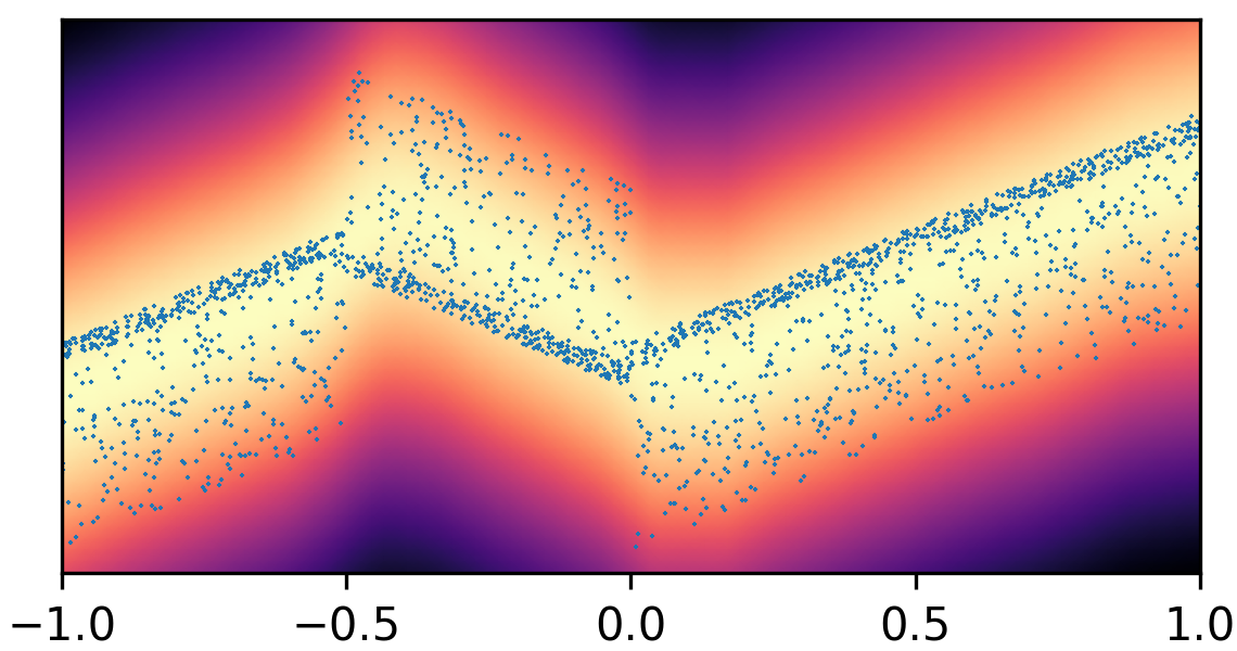
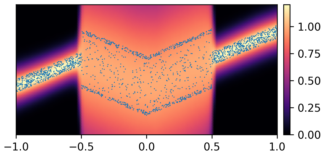
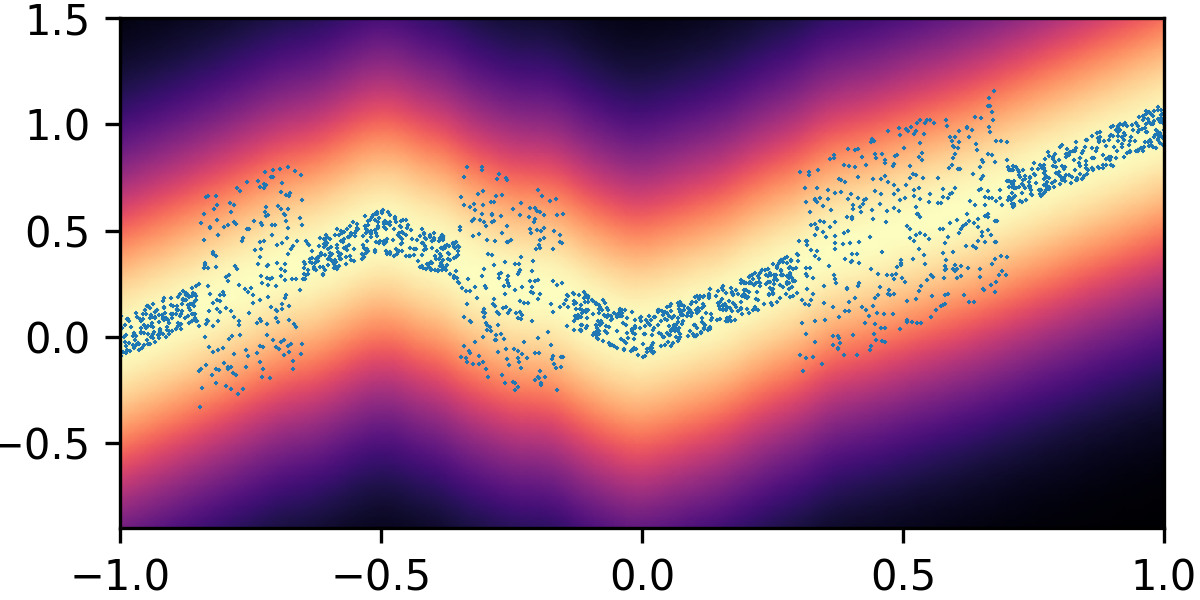
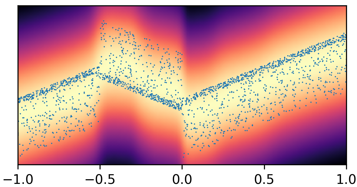
We used synthetic datasets to evaluate the predictive density estimated by each method against the ground truth. The input variable $x$ was one-dimensional and uniformly distributed on $[-1,1]$ . The output variable $y$ was also one-dimensional, and its conditional median was a linear spline with respect to $x$ . We designed the noise distribution to be heteroscedastic, asymmetric, or multimodal, as shown by the blue circles in Figure 1. Training sample size varied among 1000, 2000, and 4000. Every experimental setting was repeated for 20 times.

We used a B-DeepNoise model with 4 hidden layers and 50 nodes in each layer, with the hard tanh function as the activation function. The prior distributions of the variance parameters were set to $\mathcal{IG}(0.001,0.001)$ . We used gradient descent to initialize the model parameters and drew 500 posterior samples. B-DeepNoise was compared against backpropagation (BP) with learnable predictive variance, variational inference (VI) [77], Bayesian neural networks (BNN) with Hamiltonian Monte Carlo [78], and deep ensemble (DE) [22]. The baseline methods used identical architecture as B-DeepNoise, and the hyperparameters were selected according to the original authors’ recommendations. Details of the experiments are described in Supplementary Materials.

As visualized in Figure 1, B-DeepNoise successfully captured key characteristics of the noise densities. The estimated predictive distributions identified variation in the output variance, regions with opposite directions of skewedness, and abrupt changes from unimodal to bimodal distributions. In contrast, predictive densities estimated by DE, which is the best baseline method, were mostly unimodal and symmetric and overestimated the predictive variance overall. Furthermore, the predictive densities estimated by VI were primarily homoscedastic.

To quantitatively evaluate the accuracy of the estimated predictive density functions, we numerically computed the $L_{1}$ distance between the inverse CDFs of the true and estimated predictive distributions over a grid of input values. The average estimation errors are reported in Table 1. Among all the methods, B-DeepNoise had the smallest error in all but two settings. Moreover, for all three types of noises, B-DeepNoise’s accuracy improved much faster than the baseline methods as the training sample size increased, especially on the skewed and multimodal data. These simulations illustrate the accuracy and efficiency of B-DeepNoise in learning complex predictive density functions.

3.2 Experiments on Real Data

Table 2: UCI experiment results on testing data for B-DeepNoise and baseline methods.

Dataset	BP	VI	BNN	DMC	DE	B-DeepNoise
Root Mean Squared Error (RMSE)
Yacht Hydrodynamics	3.09 $\pm$ 1.28	2.10 $\pm$ 0.43	0.68 $\pm$ 0.04	3.30 $\pm$ 1.14	2.02 $\pm$ 0.76	0.64 $\pm$ 0.32
Boston Housing	3.36 $\pm$ 1.05	2.75 $\pm$ 0.67	5.60 $\pm$ 0.12	3.10 $\pm$ 0.88	3.16 $\pm$ 1.11	2.84 $\pm$ 0.69
Energy Efficiency	2.45 $\pm$ 0.32	0.68 $\pm$ 0.09	10.31 $\pm$ 0.16	1.46 $\pm$ 0.18	2.56 $\pm$ 0.32	0.45 $\pm$ 0.07
Concrete Strength	5.98 $\pm$ 0.62	4.68 $\pm$ 0.52	17.14 $\pm$ 0.31	6.11 $\pm$ 0.47	5.45 $\pm$ 0.55	4.54 $\pm$ 0.46
Wine Quality	0.64 $\pm$ 0.05	0.66 $\pm$ 0.07	0.69 $\pm$ 0.01	0.62 $\pm$ 0.04	0.62 $\pm$ 0.04	0.63 $\pm$ 0.04
Kin8nm	0.08 $\pm$ 0.00	0.09 $\pm$ 0.00	0.16 $\pm$ 0.00	2.27 $\pm$ 0.23	0.07 $\pm$ 0.00	0.07 $\pm$ 0.00
Power Plant	4.02 $\pm$ 0.15	3.89 $\pm$ 0.20	17.74 $\pm$ 0.10	4.12 $\pm$ 0.15	3.98 $\pm$ 0.15	3.62 $\pm$ 0.18
Naval Propulsion	0.00 $\pm$ 0.00	0.00 $\pm$ 0.00	0.02 $\pm$ 0.00	509.93 $\pm$ 0.00	0.00 $\pm$ 0.00	0.00 $\pm$ 0.00
Protein Structure	4.08 $\pm$ 0.06	4.35 $\pm$ 0.09	6.31 $\pm$ 0.05	4.02 $\pm$ 0.04	3.91 $\pm$ 0.03	3.64 $\pm$ 0.03
Negative Log Likelihood (NLL)
Yacht Hydrodynamics	1.39 $\pm$ 0.33	2.64 $\pm$ 0.04	0.88 $\pm$ 0.08	2.29 $\pm$ 1.14	1.09 $\pm$ 0.19	0.45 $\pm$ 0.22
Boston Housing	3.01 $\pm$ 0.90	2.40 $\pm$ 0.12	3.18 $\pm$ 0.02	2.42 $\pm$ 0.88	2.37 $\pm$ 0.27	2.28 $\pm$ 0.17
Energy Efficiency	1.77 $\pm$ 0.59	1.36 $\pm$ 0.06	3.33 $\pm$ 0.01	1.79 $\pm$ 0.18	1.54 $\pm$ 0.25	0.55 $\pm$ 0.19
Concrete Strength	3.41 $\pm$ 0.47	3.03 $\pm$ 0.21	4.24 $\pm$ 0.01	3.19 $\pm$ 0.47	3.04 $\pm$ 0.22	2.84 $\pm$ 0.14
Wine Quality	2.07 $\pm$ 0.86	10.05 $\pm$ 4.03	1.02 $\pm$ 0.01	0.92 $\pm$ 0.04	1.03 $\pm$ 0.25	0.95 $\pm$ 0.09
Kin8nm	-1.01 $\pm$ 0.21	1.67 $\pm$ 0.44	-0.40 $\pm$ 0.03	-0.92 $\pm$ 0.02	-1.30 $\pm$ 0.04	-1.31 $\pm$ 0.04
Power Plant	2.81 $\pm$ 0.06	2.92 $\pm$ 0.10	4.18 $\pm$ 0.01	2.80 $\pm$ 0.03	2.77 $\pm$ 0.05	2.70 $\pm$ 0.06
Naval Propulsion	-4.67 $\pm$ 1.29	-7.19 $\pm$ 0.48	-2.09 $\pm$ 0.03	-4.10 $\pm$ 0.03	-5.15 $\pm$ 0.21	-7.25 $\pm$ 0.07
Protein Structure	2.80 $\pm$ 0.19	3.25 $\pm$ 0.03	3.25 $\pm$ 0.01	2.77 $\pm$ 0.01	2.54 $\pm$ 0.05	2.65 $\pm$ 0.09
Width of 95% Empirical Prediction Intervals (WEPI-95)
Yacht Hydrodynamics	2.63 $\pm$ 1.17	6.01 $\pm$ 1.72	2.37 $\pm$ 0.20	$\infty$ $\pm$ NA	2.34 $\pm$ 0.91	0.45 $\pm$ 0.22
Boston Housing	$\infty$ $\pm$ NA	9.81 $\pm$ 1.60	20.94 $\pm$ 0.64	10.51 $\pm$ 1.90	$\infty$ $\pm$ NA	2.28 $\pm$ 0.17
Energy Efficiency	3.70 $\pm$ 1.05	2.60 $\pm$ 0.46	16.79 $\pm$ 0.54	6.28 $\pm$ 1.14	3.55 $\pm$ 0.79	0.55 $\pm$ 0.19
Concrete Strength	$\infty$ $\pm$ NA	$\infty$ $\pm$ NA	56.51 $\pm$ 0.53	25.45 $\pm$ 2.68	17.40 $\pm$ 3.02	2.84 $\pm$ 0.14
Wine Quality	$\infty$ $\pm$ NA	$\infty$ $\pm$ NA	2.85 $\pm$ 0.05	$\infty$ $\pm$ NA	2.88 $\pm$ 0.34	0.95 $\pm$ 0.09
Kin8nm	0.30 $\pm$ 0.02	$\infty$ $\pm$ NA	0.61 $\pm$ 0.01	11.24 $\pm$ 1.11	0.26 $\pm$ 0.01	0.26 $\pm$ 0.01
Power Plant	14.89 $\pm$ 0.52	15.28 $\pm$ 0.76	53.66 $\pm$ 0.63	$\infty$ $\pm$ NA	14.76 $\pm$ 0.56	13.90 $\pm$ 0.62
Naval Propulsion	$\infty$ $\pm$ NA	0.00 $\pm$ 0.00	0.05 $\pm$ 0.00	2548.88 $\pm$ 0.00	0.00 $\pm$ 0.00	0.00 $\pm$ 0.00
Protein Structure	16.32 $\pm$ 0.63	$\infty$ $\pm$ NA	23.23 $\pm$ 0.27	$\infty$ $\pm$ NA	14.06 $\pm$ 0.37	11.90 $\pm$ 0.19

We applied B-DeepNoise and baselines methods to nine UCI regression datasets [79]. Experiment setup was similar to [46, 22], where each dataset was randomly split into training and testing sets for 20 times in all the datasets except Protein Structure, where only 5 random splits were made due to the larger sample size. Prediction accuracy was measured by the testing root mean squared error (RMSE) of the predictive mean, and the predictive distribution was assessed by the testing negative log likelihood (NLL). For efficiency of UQ, since the 95% prediction intervals might be miscalibrated, we computed the 95% empirical prediction intervals (EPIs), defined as the $x$ % prediction intervals with minimal $x$ that cover at least 95% of the observed testing outcomes. Then UQ efficiency was evaluated by the average width of the 95% EPIs (WEPI-95). We compared B-DeepNoise against backpropagation (BP) with learnable predictive variance, variational inference (VI), Bayesian Neural Network (BNN) with Hamiltonian Monte Carlo, Dropout Monte Carlo (DMC), and Deep Ensemble (DE). All methods used 4 hidden layers with 50 nodes per layer, with the hard tanh activation function. Experiment setup is similar to that of simulation studies. (See Supplementary Materials for details.)

Table 2 shows the results on the testing data. Compared to the baseline methods, B-DeepNoise had the least RMSE on all except two datasets, indicating a superior prediction accuracy. Moreover, B-DeepNoise’s predictive distribution was also overall more accurate than the other methods, since the NLL of B-DeepNoise was the smallest on all except two datasets. Furthermore, the high UQ efficiency of B-DeepNoise was demonstrated by its uniformly narrowest WEPI-95. In comparison, the baseline methods not only had significantly larger WEPI-95s, but also could not produce valid 95% EPIs at all on some of the datasets (as indicated by $\infty$ in Table 2), since even their 100% prediction intervals could not cover at least 95% of the testing outcomes. In addition, B-DeepNoise’s performance was overall more stable than the baseline methods, as reflected by its generally smaller standard errors of all the metrics. In sum, the experiments on the UCI datasets demonstrated the superior DR accuracy and UQ efficiency of B-DeepNoise compared to existing methods.

4 Neuroimaging-Based Prediction of General Intelligence for Adolescents

We demonstrate the usefulness of B-DeepNoise in scientific studies by applying it to the neuroimaging data in the Adolescent Brain Cognitive Development (ABCD) Study [80, 81]. The dataset contains 1191 subjects aged between 9 and 10 years old, recruited from multiple study sites in the United States. For every subject, the data contain general intelligence score (g-score) [82, 83], 2-back task score [84], general psychopathology factor [85, 86, 87], demographic information (including age, sex, parental education level, household marital status, household income, and ethnic backgrounds), and brain functional magnetic resonance imagings (fMRIs). In this study, each subject is asked to participate in the 2-back task, which is a functional assessment task designed to engage memory regulation processes, and a score is produced at the end to summarize the performance. In addition, brain fMRI scans are acquired at resting state and during the 2-back task. The brain fMRI images in our dataset, which have resolution $61\times 73\times 61$ , are obtained by contrasting the resting state scans and the task-active scans with minimal processing. These images reflect brain activity that is stimulated by the 2-back task.

The goal of our analysis is to predict the g-score by using the other features as predictors. To this end, we train a B-DeepNoise model by using the imaging and non-imaging features. In order to provide biological interpretations, we segmented the whole brain volume into 90 regions according to the automated anatomical labeling (AAL) atlas [88]. Then inside each region, we computed the mean of the imaging values for each subject. In total, we had 90 imaging predictors and 8 non-imaging predictors. We randomly selected 90% of the samples for training and the rest for testing. The hyperparameters for B-DeepNoise are similar to those in the analysis of the UCI datasets See Supplementary Materials for details of the experiment setup.

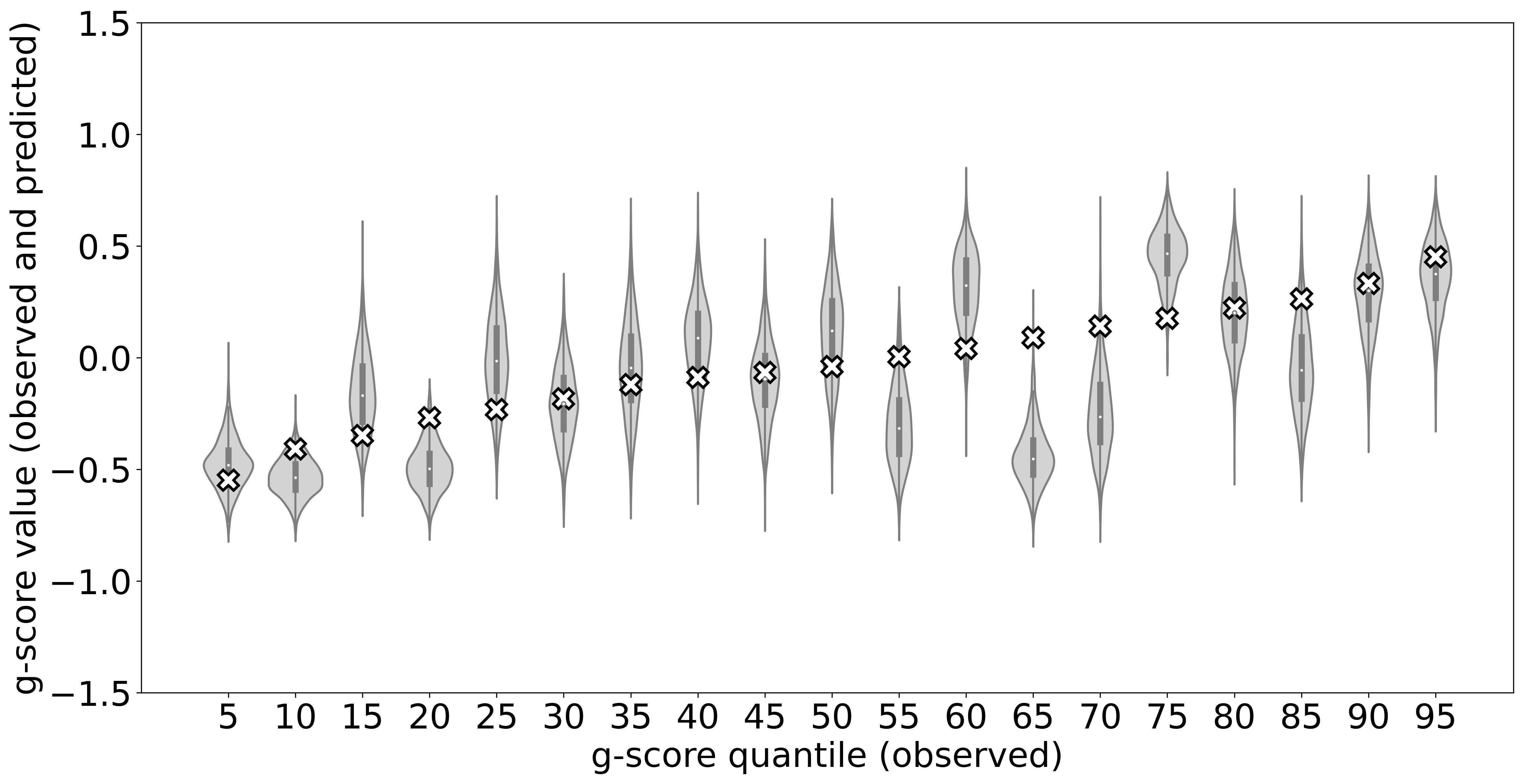
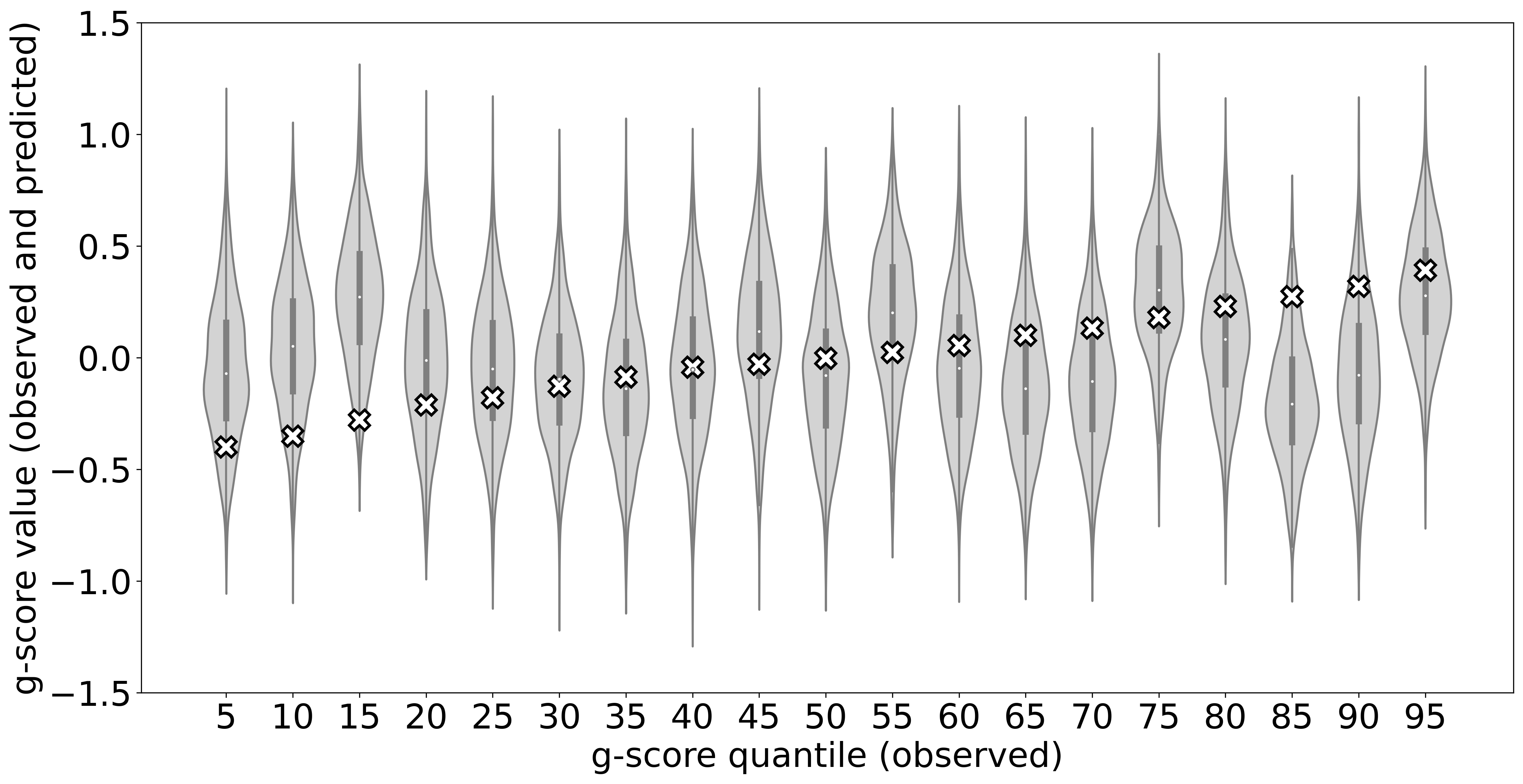
To illustrate the predictive density functions learned by B-DeepNoise, we selected 19 testing subjects that correspond to the 5%, 10%, …, 90%, 95% quantiles of the observed g-score. The results are shown in Figure 2(a). The prediction distributions estimated by B-DeepNoise have successfully covered the observed outcomes, with only a couple of samples located near the tails of the predictive distributions. To assess B-DeepNoise’s UQ efficiency, we removed the imaging predictors and refit the model with the non-imaging predictors only. As shown in Figure 2(b), when the imaging information was not available, B-DeepNoise widened the prediction intervals to account for the higher degree of uncertainty. In contrast, the predictive densities in the imaging-included model are not only more concentrated but also exhibited greater magnitude of heteroscedasticity and skewedness. These results indicate that B-DeepNoise is able to appropriately adjust the predictive density to reflect its individualized degree of confidence in its predictions.

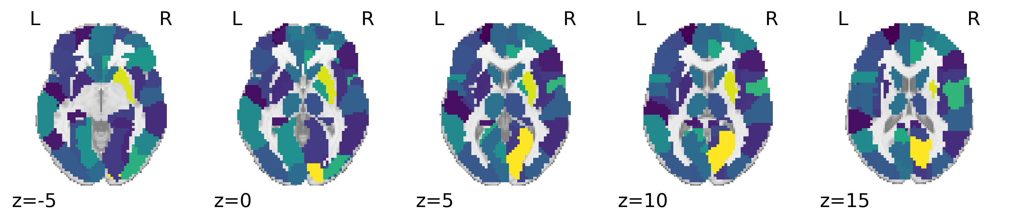
Furthermore, we investigated the most influential features on the predictive mean of the g-score. Then influence of a feature on the predictive mean is measured by the average absolute value of the gradient of the predictive mean with respect to the feature in the B-DeepNoise model. First of all, the 2-back task score had the highest influence ( $1.32$ ) on the predicted mean g-score, and the magnitude of influence was much higher than the other features ( $<0.63$ , see Supplementary Materials). This result is consistent with the current understanding that memory is a one of the major components that encompass cognitive abilities [89]. The rest of the most influential features were primarily imaging features (see Figure 3 for the influence of brain regions on predicted g-scores), and many of the corresponding brain regions have been well studied for their associations with general intelligence in existing studies. To name a few, bilateral calcarine is associated with the intelligence quotient (IQ) of children and adolescents [90]; putamen has been identified with verbal IQ in healthy adults [91]; the right paracentral lobule has been found to be associated with functioning decline in at-risk mental state patients [92]. Overall, neuroimaging regions that are the most influential for B-DeepNoise’s predicted mean g-score are supported by existing findings in the literature.

5 Discussion

In this work, we have presented B-DeepNoise, a Bayesian nonparametric model capable of DR and UQ. Intuitively, we generalize standard DNNs and BNNs by extending the random noise variables from the output layer to all the hidden layers. By iteratively composing latent random noise with linear and nonlinear transformations in the network, B-DeepNoise can learn highly complex predictive density functions. Moreover, the addition of the latent noise leads to closed-form full conditional posterior distributions of the model parameters, which we exploit to develop a Gibbs sampling algorithm for simulating the posterior distribution without relying on computationally intensive MH steps. Furthermore, we have derived theoretical properties of B-DeepNoise regarding its predictive density and variance propagation. Simulations have demonstrated B-DeepNoise’s capacity in approximating heteroscedastic, asymmetric, and multimodal predictive densities. As shown by the analysis of real benchmark datasets, compared to existing methods, B-DeepNoise not only has more accurate predictive means and predictive densities but is also more efficient in uncertainty quantification. Finally, we applied B-DeepNoise to predict genera intelligence by using neuroimaging and non-imaging in the ABCD study.

In this work, we have focused on estimating the conditional predictive densities of the output given the input, but we have not considered the marginal densities of the input. In the future, we plan on including the marginal distributions as a part of our DR and UQ model. Moreover, we are also interested in developing robust frequentist methods for the B-DeepNoise model, as the current method focuses on Bayesian frameworks. Furthermore, the current version of B-DeepNoise is limited to continuous outcomes. For categorical outcomes, a softmax function can be appended to the output layer and approximated by piecewise linear functions. Then the Gibbs sampler for B-DeepNoise can be easily extended to categorical outcome variables. See Supplementary Materials for a more detailed discussion. In addition, we have yet investigated B-DeepNoise on multi-outcome data. Our model has the potential as an outcome selection method, where the goal is to differentiate predictable and unpredictable outcome variables.

References

[1] Ian Goodfellow, Yoshua Bengio, Aaron Courville, and Yoshua Bengio. Deep learning, volume 1. MIT press Cambridge, 2016.
[2] Yann LeCun, Yoshua Bengio, and Geoffrey Hinton. Deep learning. nature, 521(7553):436–444, 2015.
[3] Samira Pouyanfar, Saad Sadiq, Yilin Yan, Haiman Tian, Yudong Tao, Maria Presa Reyes, Mei-Ling Shyu, Shu-Ching Chen, and Sundaraja S Iyengar. A survey on deep learning: Algorithms, techniques, and applications. ACM Computing Surveys (CSUR), 51(5):1–36, 2018.
[4] Julius Berner, Philipp Grohs, Gitta Kutyniok, and Philipp Petersen. The modern mathematics of deep learning. arXiv preprint arXiv:2105.04026, 2021.
[5] Mariusz Bojarski, Davide Del Testa, Daniel Dworakowski, Bernhard Firner, Beat Flepp, Prasoon Goyal, Lawrence D Jackel, Mathew Monfort, Urs Muller, Jiakai Zhang, et al. End to end learning for self-driving cars. arXiv preprint arXiv:1604.07316, 2016.
[6] Sorin Grigorescu, Bogdan Trasnea, Tiberiu Cocias, and Gigel Macesanu. A survey of deep learning techniques for autonomous driving. Journal of Field Robotics, 37(3):362–386, 2020.
[7] Justin Ker, Lipo Wang, Jai Rao, and Tchoyoson Lim. Deep learning applications in medical image analysis. Ieee Access, 6:9375–9389, 2017.
[8] James Zou, Mikael Huss, Abubakar Abid, Pejman Mohammadi, Ali Torkamani, and Amalio Telenti. A primer on deep learning in genomics. Nature genetics, 51(1):12–18, 2019.
[9] Natalie Stephenson, Emily Shane, Jessica Chase, Jason Rowland, David Ries, Nicola Justice, Jie Zhang, Leong Chan, and Renzhi Cao. Survey of machine learning techniques in drug discovery. Current drug metabolism, 20(3):185–193, 2019.
[10] Ryad Zemouri, Noureddine Zerhouni, and Daniel Racoceanu. Deep learning in the biomedical applications: Recent and future status. Applied Sciences, 9(8):1526, 2019.
[11] Edmon Begoli, Tanmoy Bhattacharya, and Dimitri Kusnezov. The need for uncertainty quantification in machine-assisted medical decision making. Nature Machine Intelligence, 1(1):20–23, 2019.
[12] Dario Amodei, Chris Olah, Jacob Steinhardt, Paul Christiano, John Schulman, and Dan Mané. Concrete problems in ai safety. arXiv preprint arXiv:1606.06565, 2016.
[13] Xiaoqian Jiang, Melanie Osl, Jihoon Kim, and Lucila Ohno-Machado. Calibrating predictive model estimates to support personalized medicine. Journal of the American Medical Informatics Association, 19(2):263–274, 2012.
[14] Christian Leibig, Vaneeda Allken, Murat Seçkin Ayhan, Philipp Berens, and Siegfried Wahl. Leveraging uncertainty information from deep neural networks for disease detection. Scientific reports, 7(1):1–14, 2017.
[15] David B Dunson, Natesh Pillai, and Ju-Hyun Park. Bayesian density regression. Journal of the Royal Statistical Society: Series B (Statistical Methodology), 69(2):163–183, 2007.
[16] Moloud Abdar, Farhad Pourpanah, Sadiq Hussain, Dana Rezazadegan, Li Liu, Mohammad Ghavamzadeh, Paul Fieguth, Xiaochun Cao, Abbas Khosravi, U Rajendra Acharya, et al. A review of uncertainty quantification in deep learning: Techniques, applications and challenges. Information Fusion, 76:243–297, 2021.
[17] Niclas Ståhl, Göran Falkman, Alexander Karlsson, and Gunnar Mathiason. Evaluation of uncertainty quantification in deep learning. In International Conference on Information Processing and Management of Uncertainty in Knowledge-Based Systems, pages 556–568. Springer, 2020.
[18] João Caldeira and Brian Nord. Deeply uncertain: comparing methods of uncertainty quantification in deep learning algorithms. Machine Learning: Science and Technology, 2(1):015002, 2020.
[19] Yinhao Zhu, Nicholas Zabaras, Phaedon-Stelios Koutsourelakis, and Paris Perdikaris. Physics-constrained deep learning for high-dimensional surrogate modeling and uncertainty quantification without labeled data. Journal of Computational Physics, 394:56–81, 2019.
[20] Christopher M Bishop. Mixture density networks. 1994.
[21] Christopher M Bishop and Nasser M Nasrabadi. Pattern recognition and machine learning, volume 4. Springer, 2006.
[22] Balaji Lakshminarayanan, Alexander Pritzel, and Charles Blundell. Simple and scalable predictive uncertainty estimation using deep ensembles. arXiv preprint arXiv:1612.01474, 2016.
[23] Jing Lei and Larry Wasserman. Distribution-free prediction bands for non-parametric regression. Journal of the Royal Statistical Society: Series B (Statistical Methodology), 76(1):71–96, 2014.
[24] Tim Pearce, Alexandra Brintrup, Mohamed Zaki, and Andy Neely. High-quality prediction intervals for deep learning: A distribution-free, ensembled approach. In International conference on machine learning, pages 4075–4084. PMLR, 2018.
[25] Yaniv Romano, Evan Patterson, and Emmanuel Candes. Conformalized quantile regression. Advances in neural information processing systems, 32, 2019.
[26] Natasa Tagasovska and David Lopez-Paz. Single-model uncertainties for deep learning. Advances in Neural Information Processing Systems, 32, 2019.
[27] Rui Li, Brian J Reich, and Howard D Bondell. Deep distribution regression. Computational Statistics & Data Analysis, 159:107203, 2021.
[28] David B Huberman, Brian J Reich, and Howard D Bondell. Nonparametric conditional density estimation in a deep learning framework for short-term forecasting. Environmental and Ecological Statistics, pages 1–15, 2021.
[29] David JC MacKay. Probable networks and plausible predictions-a review of practical bayesian methods for supervised neural networks. Network: computation in neural systems, 6(3):469, 1995.
[30] Radford M Neal. Bayesian learning for neural networks, volume 118. Springer Science & Business Media, 2012.
[31] Yujia Xue, Shiyi Cheng, Yunzhe Li, and Lei Tian. Reliable deep-learning-based phase imaging with uncertainty quantification. Optica, 6(5):618–629, 2019.
[32] JT Gene Hwang and A Adam Ding. Prediction intervals for artificial neural networks. Journal of the American Statistical Association, 92(438):748–757, 1997.
[33] Yuexi Wang and Veronika Rocková. Uncertainty quantification for sparse deep learning. In International Conference on Artificial Intelligence and Statistics, pages 298–308. PMLR, 2020.
[34] Yan Sun, Wenjun Xiong, and Faming Liang. Sparse deep learning: A new framework immune to local traps and miscalibration. Advances in Neural Information Processing Systems, 34, 2021.
[35] Alex Kendall and Yarin Gal. What uncertainties do we need in bayesian deep learning for computer vision? arXiv preprint arXiv:1703.04977, 2017.
[36] Pavel Izmailov, Dmitrii Podoprikhin, Timur Garipov, Dmitry Vetrov, and Andrew Gordon Wilson. Averaging weights leads to wider optima and better generalization. arXiv preprint arXiv:1803.05407, 2018.
[37] David M Blei, Alp Kucukelbir, and Jon D McAuliffe. Variational inference: A review for statisticians. Journal of the American statistical Association, 112(518):859–877, 2017.
[38] Diederik P Kingma and Max Welling. Auto-encoding variational bayes. arXiv preprint arXiv:1312.6114, 2013.
[39] Stephan Mandt, Matthew D Hoffman, and David M Blei. Stochastic gradient descent as approximate bayesian inference. Journal of Machine Learning Research, 18:1–35, 2017.
[40] Alex Graves. Practical variational inference for neural networks. Advances in neural information processing systems, 24, 2011.
[41] Christos Louizos and Max Welling. Structured and efficient variational deep learning with matrix gaussian posteriors. In International conference on machine learning, pages 1708–1716. PMLR, 2016.
[42] Jongseok Lee, Matthias Humt, Jianxiang Feng, and Rudolph Triebel. Estimating model uncertainty of neural networks in sparse information form. In International Conference on Machine Learning, pages 5702–5713. PMLR, 2020.
[43] Danilo Rezende and Shakir Mohamed. Variational inference with normalizing flows. In International conference on machine learning, pages 1530–1538. PMLR, 2015.
[44] Christos Louizos and Max Welling. Multiplicative normalizing flows for variational bayesian neural networks. In International Conference on Machine Learning, pages 2218–2227. PMLR, 2017.
[45] Nitish Srivastava, Geoffrey Hinton, Alex Krizhevsky, Ilya Sutskever, and Ruslan Salakhutdinov. Dropout: a simple way to prevent neural networks from overfitting. The journal of machine learning research, 15(1):1929–1958, 2014.
[46] Yarin Gal and Zoubin Ghahramani. Dropout as a bayesian approximation: Representing model uncertainty in deep learning. In international conference on machine learning, pages 1050–1059. PMLR, 2016.
[47] Dmitry Molchanov, Arsenii Ashukha, and Dmitry Vetrov. Variational dropout sparsifies deep neural networks. In International Conference on Machine Learning, pages 2498–2507. PMLR, 2017.
[48] Sergey Ioffe and Christian Szegedy. Batch normalization: Accelerating deep network training by reducing internal covariate shift. In International conference on machine learning, pages 448–456. PMLR, 2015.
[49] Mattias Teye, Hossein Azizpour, and Kevin Smith. Bayesian uncertainty estimation for batch normalized deep networks. In International Conference on Machine Learning, pages 4907–4916. PMLR, 2018.
[50] Charles Blundell, Julien Cornebise, Koray Kavukcuoglu, and Daan Wierstra. Weight uncertainty in neural network. In International Conference on Machine Learning, pages 1613–1622. PMLR, 2015.
[51] José Miguel Hernández-Lobato and Ryan Adams. Probabilistic backpropagation for scalable learning of bayesian neural networks. In International conference on machine learning, pages 1861–1869. PMLR, 2015.
[52] Siddhartha Chib and Edward Greenberg. Understanding the metropolis-hastings algorithm. The american statistician, 49(4):327–335, 1995.
[53] David B Hitchcock. A history of the metropolis–hastings algorithm. The American Statistician, 57(4):254–257, 2003.
[54] Christophe Andrieu and Johannes Thoms. A tutorial on adaptive mcmc. Statistics and computing, 18(4):343–373, 2008.
[55] Florian Wenzel, Kevin Roth, Bastiaan S Veeling, Jakub Świątkowski, Linh Tran, Stephan Mandt, Jasper Snoek, Tim Salimans, Rodolphe Jenatton, and Sebastian Nowozin. How good is the bayes posterior in deep neural networks really? arXiv preprint arXiv:2002.02405, 2020.
[56] Andrew Gordon Wilson and Pavel Izmailov. Bayesian deep learning and a probabilistic perspective of generalization. arXiv preprint arXiv:2002.08791, 2020.
[57] Max Welling and Yee W Teh. Bayesian learning via stochastic gradient langevin dynamics. In Proceedings of the 28th international conference on machine learning (ICML-11), pages 681–688. Citeseer, 2011.
[58] Tianqi Chen, Emily Fox, and Carlos Guestrin. Stochastic gradient hamiltonian monte carlo. In International conference on machine learning, pages 1683–1691. PMLR, 2014.
[59] Changyou Chen, David Carlson, Zhe Gan, Chunyuan Li, and Lawrence Carin. Bridging the gap between stochastic gradient mcmc and stochastic optimization. In Artificial Intelligence and Statistics, pages 1051–1060. PMLR, 2016.
[60] Tung-Yu Wu, YX Rachel Wang, and Wing H Wong. Mini-batch metropolis–hastings with reversible sgld proposal. Journal of the American Statistical Association, pages 1–9, 2020.
[61] Faming Liang, Jinsu Kim, and Qifan Song. A bootstrap metropolis–hastings algorithm for bayesian analysis of big data. Technometrics, 58(3):304–318, 2016.
[62] Laurent Valentin Jospin, Hamid Laga, Farid Boussaid, Wray Buntine, and Mohammed Bennamoun. Hands-on bayesian neural networks—a tutorial for deep learning users. IEEE Computational Intelligence Magazine, 17(2):29–48, 2022.
[63] Stuart Geman and Donald Geman. Stochastic relaxation, gibbs distributions, and the bayesian restoration of images. IEEE Transactions on pattern analysis and machine intelligence, (6):721–741, 1984.
[64] Alan E Gelfand and Adrian FM Smith. Sampling-based approaches to calculating marginal densities. Journal of the American statistical association, 85(410):398–409, 1990.
[65] Gareth O Roberts and Adrian FM Smith. Simple conditions for the convergence of the gibbs sampler and metropolis-hastings algorithms. Stochastic processes and their applications, 49(2):207–216, 1994.
[66] Alan E Gelfand. Gibbs sampling. Journal of the American statistical Association, 95(452):1300–1304, 2000.
[67] Zhonghui You, Jinmian Ye, Kunming Li, Zenglin Xu, and Ping Wang. Adversarial noise layer: Regularize neural network by adding noise. In 2019 IEEE International Conference on Image Processing (ICIP), pages 909–913. IEEE, 2019.
[68] Caglar Gulcehre, Marcin Moczulski, Misha Denil, and Yoshua Bengio. Noisy activation functions. In International conference on machine learning, pages 3059–3068. PMLR, 2016.
[69] Joonho Lee, Kumar Shridhar, Hideaki Hayashi, Brian Kenji Iwana, Seokjun Kang, and Seiichi Uchida. Probact: A probabilistic activation function for deep neural networks. arXiv preprint arXiv:1905.10761, 5:13, 2019.
[70] Yan Sun and Faming Liang. A kernel-expanded stochastic neural network. Journal of the Royal Statistical Society: Series B (Statistical Methodology), n/a(n/a), 2022.
[71] Kostantinos N Plataniotis and Dimitris Hatzinakos. Gaussian mixtures and their applications to signal processing. In Advanced signal processing handbook, pages 89–124. CRC Press, 2017.
[72] Craig Calcaterra and Axel Boldt. Approximating with gaussians. arXiv preprint arXiv:0805.3795, 2008.
[73] Franco Scarselli and Ah Chung Tsoi. Universal approximation using feedforward neural networks: A survey of some existing methods, and some new results. Neural networks, 11(1):15–37, 1998.
[74] Dmitry Yarotsky. Error bounds for approximations with deep relu networks. Neural Networks, 94:103–114, 2017.
[75] Yulong Lu and Jianfeng Lu. A universal approximation theorem of deep neural networks for expressing probability distributions. Advances in Neural Information Processing Systems, 33, 2020.
[76] Andrew L Maas, Awni Y Hannun, Andrew Y Ng, et al. Rectifier nonlinearities improve neural network acoustic models. In Proc. icml, volume 30, page 3. Citeseer, 2013.
[77] Hippolyt Ritter and Theofanis Karaletsos. Tyxe: Pyro-based bayesian neural nets for pytorch. Proceedings of Machine Learning and Systems, 4, 2022.
[78] Radford M Neal et al. Mcmc using hamiltonian dynamics. Handbook of markov chain monte carlo, 2(11):2, 2011.
[79] Dheeru Dua and Casey Graff. UCI machine learning repository, 2017.
[80] BJ Casey, Tariq Cannonier, May I Conley, Alexandra O Cohen, Deanna M Barch, Mary M Heitzeg, Mary E Soules, Theresa Teslovich, Danielle V Dellarco, Hugh Garavan, et al. The adolescent brain cognitive development (abcd) study: imaging acquisition across 21 sites. Developmental cognitive neuroscience, 32:43–54, 2018.
[81] Daiwei Zhang, Lexin Li, Chandra Sripada, and Jian Kang. Image response regression via deep neural networks. arXiv preprint arXiv:2006.09911, 2020.
[82] Julien Dubois, Paola Galdi, Lynn K Paul, and Ralph Adolphs. A distributed brain network predicts general intelligence from resting-state human neuroimaging data. Philosophical Transactions of the Royal Society B: Biological Sciences, 373(1756):20170284, 2018.
[83] Andrew O’Shea, Ronald Cohen, Eric C Porges, Nicole R Nissim, and Adam J Woods. Cognitive aging and the hippocampus in older adults. Frontiers in aging neuroscience, 8:298, 2016.
[84] Alexandra O Cohen, Kaitlyn Breiner, Laurence Steinberg, Richard J Bonnie, Elizabeth S Scott, Kim Taylor-Thompson, Marc D Rudolph, Jason Chein, Jennifer A Richeson, Aaron S Heller, et al. When is an adolescent an adult? assessing cognitive control in emotional and nonemotional contexts. Psychological Science, 27(4):549–562, 2016.
[85] Avshalom Caspi, Renate M Houts, Daniel W Belsky, Sidra J Goldman-Mellor, HonaLee Harrington, Salomon Israel, Madeline H Meier, Sandhya Ramrakha, Idan Shalev, Richie Poulton, et al. The p factor: one general psychopathology factor in the structure of psychiatric disorders? Clinical psychological science, 2(2):119–137, 2014.
[86] Charles S Carver, Sheri L Johnson, and Kiara R Timpano. Toward a functional view of the p factor in psychopathology. Clinical Psychological Science, 5(5):880–889, 2017.
[87] Aja Louise Murray, Manuel Eisner, and Denis Ribeaud. The development of the general factor of psychopathology ‘p factor’through childhood and adolescence. Journal of abnormal child psychology, 44(8):1573–1586, 2016.
[88] Nathalie Tzourio-Mazoyer, Brigitte Landeau, Dimitri Papathanassiou, Fabrice Crivello, Olivier Etard, Nicolas Delcroix, Bernard Mazoyer, and Marc Joliot. Automated anatomical labeling of activations in spm using a macroscopic anatomical parcellation of the mni mri single-subject brain. Neuroimage, 15(1):273–289, 2002.
[89] Wesley K Thompson, Deanna M Barch, James M Bjork, Raul Gonzalez, Bonnie J Nagel, Sara Jo Nixon, and Monica Luciana. The structure of cognition in 9 and 10 year-old children and associations with problem behaviors: Findings from the abcd study’s baseline neurocognitive battery. Developmental cognitive neuroscience, 36:100606, 2019.
[90] Emily Kilroy, Collin Y Liu, Lirong Yan, Yoon Chun Kim, Mirella Dapretto, Mario F Mendez, and Danny JJ Wang. Relationships between cerebral blood flow and iq in typically developing children and adolescents. Journal of cognitive science, 12(2):151, 2011.
[91] Rachael G Grazioplene, Sephira G. Ryman, Jeremy R Gray, Aldo Rustichini, Rex E Jung, and Colin G DeYoung. Subcortical intelligence: Caudate volume predicts iq in healthy adults. Human brain mapping, 36(4):1407–1416, 2015.
[92] Daiki Sasabayashi, Yoichiro Takayanagi, Tsutomu Takahashi, Shimako Nishiyama, Yuko Mizukami, Naoyuki Katagiri, Naohisa Tsujino, Takahiro Nemoto, Atsushi Sakuma, Masahiro Katsura, et al. Reduced cortical thickness of the paracentral lobule in at-risk mental state individuals with poor 1-year functional outcomes. Translational psychiatry, 11(1):1–9, 2021.

Appendix A Gibbs Sampling Algorithm for B-DeepNoise

Theorem 1 provides the full conditional posterior distribution of the pre-activation latent noise variables. In Proposition 5, we derive the counterparts for the other model parameters, which are necessary for developing a complete Gibbs sampling algorithm for B-DeepNoise.

Proposition 5.

Model parameters $\bm{u}^{(n)}_{l}$ , $\bm{\beta}_{l},\bm{\gamma}_{l}$ , $\bm{\rho}^{2}_{l},\bm{\xi}^{2}_{l}$ , $\bm{\tau}^{2}_{l},\bm{\sigma}^{2}_{l}$ have the following full conditional posterior distributions:

Post-activation latent random noise:

\displaystyle\bm{u}^{(n)}_{l}\Bigm{|}\mathrm{rest}\sim\mathcal{N}(\bm{\mu}_{\text{post},l,n},\bm{\Sigma}_{\text{post},l,n}),

(7)

where

	$\displaystyle\bm{\mu}_{\text{post},l,n}=$	$\displaystyle(\bm{\beta}_{l}\bm{\beta}_{l}^{\top}+\tilde{\bm{\Sigma}}^{-1}_{\text{post},l,n})^{-1}[\tilde{\bm{\Sigma}}^{-1}_{\text{post},l,n}h(\bm{v}_{l-1}^{(n)})+\bm{\beta}_{l}^{\top}(\bm{v}_{l}^{(n)}-\bm{\gamma}_{l})]$
	$\displaystyle\bm{\Sigma}_{\text{post},l,n}=$	$\displaystyle(\bm{\beta}_{l}^{\top}\operatorname{diag}[\bm{\tau}^{-2}_{l}]\bm{\beta}_{l}+\tilde{\bm{\Sigma}}^{-1}_{\text{post},l,n})^{-1},\qquad\tilde{\bm{\Sigma}}_{\text{post},l,n}=\operatorname{diag}[\bm{\sigma}_{l-1}^{2}]$

Weight and bias parameters:

\displaystyle(\bm{\beta}_{l,k},\gamma_{l,k})\Bigm{|}\mathrm{rest}\sim\mathcal{N}(\bm{\mu}_{\text{WB},l,k},\bm{\Sigma}_{\text{WB},l,k})

(8)

where

$\displaystyle\bm{\mu}_{\text{WB},l,k}=$	$\displaystyle(\bar{\bm{u}}_{l}\bar{\bm{u}}_{l}^{\top}+\tilde{\bm{\Sigma}}^{-1}_{\text{WB},l,k})^{-1}\bm{v}_{l,k}\bar{\bm{u}}_{l}^{\top}$
$\displaystyle\bm{\Sigma}_{\text{WB},l,k}=$	$\displaystyle(\tau^{-2}_{l,k}\bar{\bm{u}}_{l}\bar{\bm{u}}_{l}^{\top}+\tilde{\bm{\Sigma}}^{-1}_{\text{WB},l,k})^{-1},$	$\displaystyle\tilde{\bm{\Sigma}}_{\text{WB},l,k}=$	$\displaystyle\operatorname{diag}(\bm{\rho}_{l,k}^{2},\xi_{l,k}^{2})$
$\displaystyle\bar{\bm{u}}_{l}=$	$\displaystyle(\bm{u}_{l},\bm{1}),$	$\displaystyle\bm{u}_{l}=$	$\displaystyle\Big{[}\bm{u}_{l}^{(n)}\Big{]}_{n=1}^{N}$

Variance parameters:

$\displaystyle\tau^{2}_{l,k}\Bigm{\|}\mathrm{rest}\sim$	$\displaystyle\mathcal{IG}\left(a_{\text{postact}}+\frac{1}{2}N,\;b_{\text{postact}}+\frac{1}{2}\\|\bm{v}_{l,k}-\bm{\beta}_{l,k}^{\top}\bm{u}_{l}-\gamma_{l,k}\\|_{2}^{2}\right)$	(9)
$\displaystyle\sigma^{2}_{l,k}\Bigm{\|}\mathrm{rest}\sim$	$\displaystyle\mathcal{IG}\left(a_{\text{preact}}+\frac{1}{2}N,\;b_{\text{preact}}+\frac{1}{2}\\|\bm{u}_{l+1,k}-h(\bm{v}_{l,k})\\|_{2}^{2}\right)$	(10)
$\displaystyle\rho^{2}_{l,k,k^{\prime}}\Bigm{\|}\mathrm{rest}\sim$	$\displaystyle\mathcal{IG}\left(a_{\text{weight}}+\frac{1}{2},\;b_{\text{weight}}+\frac{1}{2}\beta_{l,k,k^{\prime}}^{2}\right)$	(11)
$\displaystyle\xi^{2}_{l,k}\Bigm{\|}\mathrm{rest}\sim$	$\displaystyle\mathcal{IG}\left(a_{\text{bias}}+\frac{1}{2},\;b_{\text{bias}}+\frac{1}{2}\gamma_{l,k}^{2}\right)$	(12)

where

\bm{v}_{l,k}=\Big{[}v_{l,k}^{(n)}\Big{]}_{n=1}^{N},\qquad\bm{u}_{l,k}=\Big{[}u_{l,k}^{(n)}\Big{]}_{n=1}^{N},\qquad\bm{u}_{l}=\Big{[}\bm{u}_{l}^{(n)}\Big{]}_{n=1}^{N}

The Gibbs Sampling algorithm for B-DeepNoise is presented in Algorithm 1.

Input: training features and targets

[\bm{x}^{(n)},\bm{y}^{(n)}]_{n=1}^{N_{\mathrm{train}}}

, testing features

[\bm{x}^{(n)}]_{n=1}^{N_{\mathrm{test}}}

, number of posterior samples

M

, number of realizations of the predictive distribution

R

Output: posterior predictive samples for testing targets

[[[\hat{\bm{y}}^{(n)}_{m,r}]_{r=1}^{R}]_{m=1}^{M}]_{n=1}^{N_{\mathrm{test}}}

Randomly initialize

[\bm{\beta}_{l}]_{l=0}^{L},\;[\bm{\gamma}_{l}]_{l=0}^{L},\;[\bm{\tau}^{2}_{l}]_{l=0}^{L},\;[\bm{\sigma}^{2}_{l}]_{l=0}^{L},\;[[\bm{u}^{(n)}_{l}]_{l=1}^{L}]_{n=1}^{N_{\mathrm{train}}},\;[[\bm{v}^{(n)}_{l}]_{l=0}^{L-1}]_{n=1}^{N_{\mathrm{train}}}

;

[\bm{u}^{(n)}_{0}]_{n=1}^{N_{\mathrm{train}}}\leftarrow[\bm{x}^{(n)}]_{n=1}^{N_{\mathrm{train}}}

[\bm{v}^{(n)}_{L}]_{n=1}^{N_{\mathrm{train}}}\leftarrow[\bm{y}^{(n)}]_{n=1}^{N_{\mathrm{train}}}

;

for $m\leftarrow 1,\ldots,M$ do

for $l\leftarrow 0,\ldots,L$ do

for $n\leftarrow 1,\ldots,N_{\mathrm{train}}$ do

Sample

\bm{v}^{(n)}_{l}\mid\bm{u}^{(n)}_{l},\bm{u}^{(n)}_{l+1},\bm{\beta}_{l},\bm{\gamma}_{l},\bm{\sigma}^{2}_{l},\bm{\tau}^{2}_{l}

by Equation 6 ;

Sample

\bm{u}^{(n)}_{l+1}\mid\bm{v}^{(n)}_{l},\bm{v}^{(n)}_{l+1},\bm{\beta}_{l+1},\bm{\gamma}_{l+1},\bm{\sigma}^{2}_{l+1},\bm{\tau}^{2}_{l+1}

by Equation 7 ;

end for

Sample

\bm{\beta}_{l},\bm{\gamma}_{l}\mid\bm{u}_{l},\bm{v}_{l},\bm{\tau}^{2}_{l},\bm{\rho}^{2}_{l},\bm{\xi}^{2}_{l}

by Equation 8;

Sample

\bm{\tau}^{2}_{l},\bm{\sigma}^{2}_{l},\bm{\rho}^{2}_{l},\bm{\xi}^{2}_{l}\mid\bm{v}_{l},\bm{u}_{l},\bm{\beta}_{l},\bm{\gamma}_{l},\bm{u}_{l+1}

by Equations 9, 10, 11 and 12;

end for

\hat{\bm{\beta}}_{m}\leftarrow[\bm{\beta}_{l}]_{l=0}^{L},\;\hat{\bm{\gamma}}_{m}\leftarrow[\bm{\gamma}_{l}]_{l=0}^{L},\;\hat{\bm{\tau}}^{2}_{m}\leftarrow[\bm{\tau}^{2}_{l}]_{l=0}^{L},\;\hat{\bm{\sigma}}^{2}_{m}\leftarrow[\bm{\sigma}^{2}_{l}]_{l=0}^{L}

;

end for

for $n\leftarrow 1,\ldots,N_{\mathrm{test}}$ do

for $m\leftarrow 1,\ldots,M$ do

for $r\leftarrow 1,\ldots,R$ do

Sample

\bm{y}^{(n)}_{m}\mid\bm{x}^{(n)},\hat{\bm{\beta}}_{m},\hat{\bm{\gamma}}_{m},\hat{\bm{\tau}}^{2}_{m},\hat{\bm{\sigma}}^{2}_{m}

by Equations 5 and 4 ;

\hat{\bm{y}}^{(n)}_{m,r}\leftarrow\bm{y}^{(n)}_{m}

end for

Algorithm 1 Posterior Sampler for Bayesian Deep Noise Neural Network (B-DeepNoise)