DEM-Simulation of thin elastic membranes interacting with a granulate

The discrete element method (DEM) solves Newton’s equation for the position $\boldsymbol{r}_{i}$ and the angular orientation $\boldsymbol{\varphi}_{i}$ of each particle, $i$, of mass $m_{i}$ and tensorial moment of inertia, $\hat{J}_{i}$:

Here, $\boldsymbol{F}_{i}^{\text{ext}}$ is an external force, e.g. gravity, and $\boldsymbol{F}_{ij}$ and $\boldsymbol{M}_{ij}$ are the force and torque acting on particle $i$ due to contacts with particles $j$. There are several models for $\boldsymbol{F}_{ij}$ and $\boldsymbol{M}_{ij}$ as functions of the relative position, orientation, velocity and angular velocity of the involved particles, $i$ and $j$, for an extended discussion see, e.g., shaferForceSchemesSimulations1996 ; poschelComputationalGranularDynamics2005 ; kruggel-emdenReviewExtensionNormal2007 ; kruggel-emdenStudyTangentialForce2008 ; matuttisUnderstandingDiscreteElement2014 .

In the current paper, we focus on the description of an ambient membrane and its interaction with the granular particles. In our model, the elastically deformable membrane is modeled by mass-carrying particles that are connected by viscoelastic springs (mass-spring system, MSS). The topology of the membrane is given by a mathematical graph whose vertices and edges are represented by particles and springs, respectively.

The positions of the membrane particles (here called vertex particles), thus, describe the shape of the membrane (Fig. 1).

They are subject of Newton’s equations where the forces acting on the vertex membrane particles originate from three contributions: (a) viscoelastic stretching of the membrane, (b) moments due to bending of the membrane, and (c) interaction of granular particles with the membrane. We shall discuss these contributions in Secs. 2.3-2.5. The total force acting on the vertex particles is the sum of these three contributions.

Given two adjacent vertex particles $i,j$ at positions $\boldsymbol{\rho}_{i}$, $\boldsymbol{\rho}_{j}$ and velocities $\dot{\boldsymbol{\rho}}_{i}$, $\dot{\boldsymbol{\rho}}_{j}$, we define the relative quantities

and the unit vector

The interaction between particles $i$ and $j$ is due to linear elastic spring. Particle $i$ feels the force

which is the force of a damped harmonic oscillator, with equilibrium length $\rho_{ij}^{0}$, effective mass $m_{ij}^{\text{eff}}=m_{i}m_{j}/(m_{i}+m_{j})$, damping coefficient $\gamma$, and spring constant $k$.

To relate the spring constant, $k$, to material characteristics, we notice that each realistic membrane has a finite width, $d$, and the elasticity of the membrane material is characterized by its elastic modulus $E$. For our idealized two-dimensional membrane of vanishing thickness, one obtains the elastic constant kotMassSpringModels2017 ; ostoja-starzewskiLatticeModelsMicromechanics2002 .

To explain the description of membrane flexibility, we consider four adjacent vertex particles at positions $\boldsymbol{\rho}_{1}$, $\boldsymbol{\rho}_{2}$, $\boldsymbol{\rho}_{3}$, $\boldsymbol{\rho}_{4}$ bridsonSimulationClothingFolds2003 , see Fig. 2.

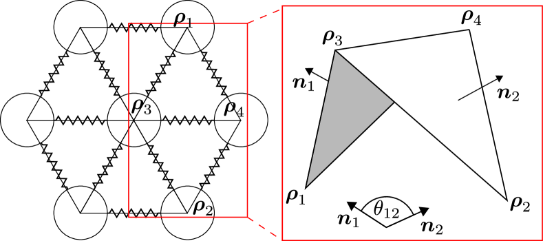
The vertex particles span two triangles with normal vectors

The corresponding angle $\theta_{12}$

characterizes the flection of the triangles, with respect to their common edge $\boldsymbol{\rho}_{43}=\boldsymbol{\rho}_{4}-\boldsymbol{\rho}_{3}$. The restoring torque counteracting the flection can be expressed by elastic and dissipative forces, $\boldsymbol{F}_{i}^{\text{el}}$, acting on the involved vertex particles, $i\in\{1,2,3,4\}$ bridsonSimulationClothingFolds2003 ,

where $k^{\text{el}}$ and $k^{\text{diss}}$ are material parameters.

The directions of the forces are linear combinations of the triangles’ normal vectors given by

Each vertex particle is involved in 6 different pairs of triangles, see Fig. 1. The total force acting on a vertex particle is, thus, the sum of the 6 corresponding forces given by Eqs. (11, 12).

For the description of the interaction between the membrane and the confined granular particles, we assume triangular patches spanned between the time dependent momentary positions of adjacent vertex particles, Fig. 3.

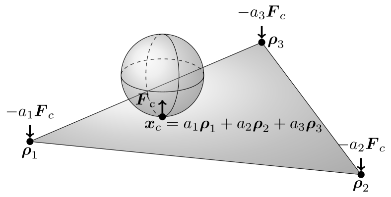
The interaction of the granular particles with the membrane is then described by contacts between the granular particles and the patches. This assures that the patches are always impenetrable disregarding of the sizes of the particles and the deformation of the membrane.

Contacts between a patch and a granular particle are classified as vertex, edge, or face contact:

In case a granular particle contacts two neighboring patches, $A$ and $B$, we chose the adequate contacts according to Tab. 1 in dependence whether these contacts are face, edge, or vertex contacts huNewAlgorithmContact2013

These selection rules do only apply if the patches $A$ and $B$ have a common edge. Otherwise, all contacts are handles regularly.

In case a granular particle contacts three neighboring patches at their common vertex, one of these contacts is selected randomly and the others are disregarded.

Contacts of the membrane with itself may be calculated from contacts between vertex particles and triangular patches.

Once the contact point is defined, we compute the force according to the specified contact law. The relative velocity of the granular particle and the membrane at the contact point which enters the force is interpolated from the velocities of the vertex particles using barycentric weights, as sketched in Fig. 3. Similarly, the obtained force is distributed to the involved vertex particles with barycentric weights $a_{1}$, $a_{2}$, $a_{3}$. The positions and velocities of the vertex particles and, thus, the dynamics of the membrane are obtained by numerical integration in the same way as the granular particles.

The above selection rule above in combination with the barycentric partition of the force leads to smooth and physically plausible forces acting on the vertex particles. huNewAlgorithmContact2013

The triaxial test is commonly used to investigate the mechanical properties of a granular sample. To that aim, the sample is placed between two parallel platens and wrapped by a cylindrical membrane, see Fig. 4.

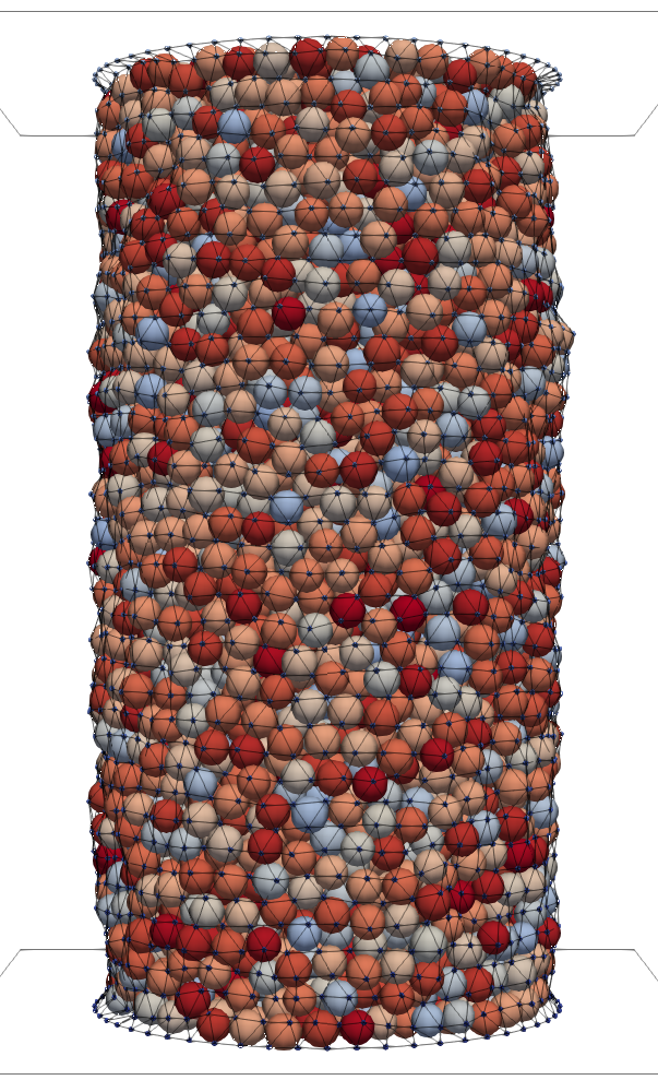
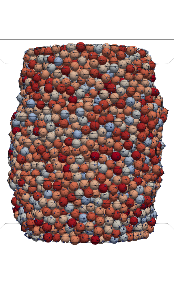
A confining stress $\sigma_{\text{c}}$ in radial direction is applied through the membrane. By controlling the initial distance $h=h_{0}$ between the platens, an initial stress $\sigma_{\text{p}}=\sigma_{\text{c}}$ is applied in axial direction. Then, the platens are displaced at constant relative velocity $\boldsymbol{v_{p}}$ to apply a strain $\epsilon=\log(h_{0}/h)$. We record the corresponding deviatoric stress $\sigma_{\text{d}}=\sigma_{\text{p}}-\sigma_{\text{c}}$.

In the simulation, we represent the platens by rigid walls and the membrane by an MSS. We place small particles at random positions inside the membrane such that they do not contact one another. To generate the initial conditions, we apply the Lubachevsky–Stillinger algorithm lubachevskyGeometricPropertiesRandom1990 . We then gradually apply an initial stress, $\sigma_{p}$, to the platens and a confining stress, $\sigma_{\text{c}}$, to the membrane. To this end, each triangular patch of area $A^{w}_{i}$ and normal unit vector $\hat{\boldsymbol{n}}^{\,w}_{i}$ is loaded with a force

where $\hat{\boldsymbol{n}}^{\,w}_{i}$ is defined such that force acts from outside the membrane to the granulate located inside. After this initialization, we displace the platens at relative velocity $\boldsymbol{v}_{\text{p}}$ and record the deviatoric stress, $\sigma_{\text{d}}$. Figure 4 shows the initial and final states of such a simulation.

To demonstrate the performance of our model, we perform simulations for two different cases:

1. 1.

   We describe the membrane by a MSS where the confining stress of the membrane is provided by contacts between vertex particles and granular particles. This approach was used before, e.g., in quDiscreteElementModelling2019 . We term this setup $\text{MSS}_{\text{particle}}$.

2. 2.

   We describe the membrane as described in Sec. 2. Here the confining stress of the membrane is provided by contacts between the granular particles and the triangular patches. We term this setup $\text{MSS}_{\text{patch}}$.

For $\text{MSS}_{\text{particle}}$, we place the vertex particles of the membrane spaced by $s=1.33\,\text{mm}$, such that the radius of a vertex particle is about $1/3$ the radius of a granular particle. This value is a trade-off between keeping the computational cost low and having a smooth membrane that prevents penetration of granular particles debonoDiscreteElementModelling2012 ; quDiscreteElementModelling2019 . For $\text{MSS}_{\text{patch}}$, we use $s=4.0\,\text{mm}$ because the membrane has a smooth surface and is impenetrable by design.

We perform the triaxial test at velocity $v_{\text{p}}=0.05\,\text{m}/\text{s}$ and confining pressure $\sigma_{\text{c}}=100\,\text{kPa}$. The material parameters are given in Tab. 2. Furthermore, we choose the parameters $\gamma\approx 0.15$, $k^{\text{el}}=10^{-3}\,\text{N/m}$ and $k^{\text{diss}}=10^{-4}\,\text{Ns/m}$. Using the initial areas of the triangles, we use Eqs. (11-16) to compute the confining forces.

We consider two different systems: case 1 – a cylinder of initial height $100\,\text{mm}$ and radius $25\,\text{mm}$, and case 2 - a cylinder of initial height $140\,\text{mm}$ and radius $35\,\text{mm}$. The numbers of particles used for the membrane and the granulate are given in Tab. 3.

Figure 5

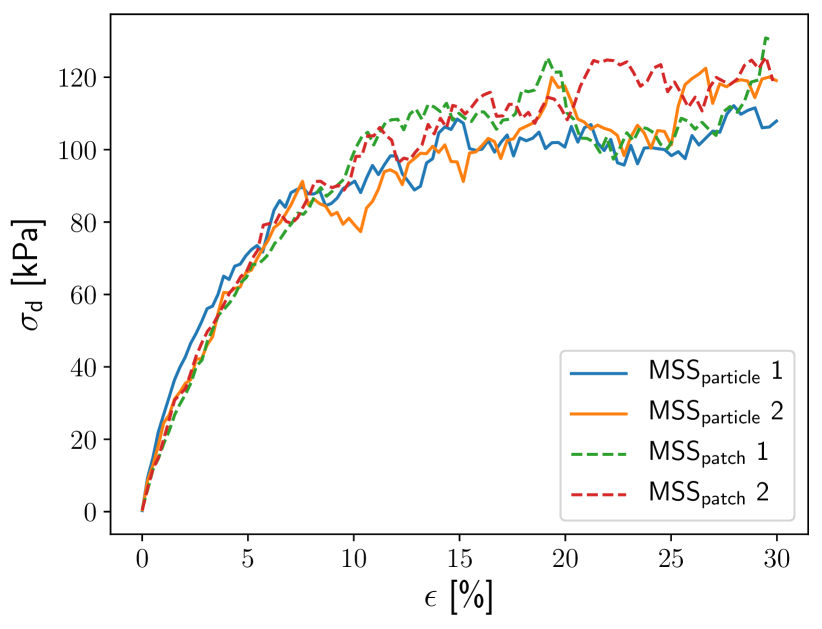
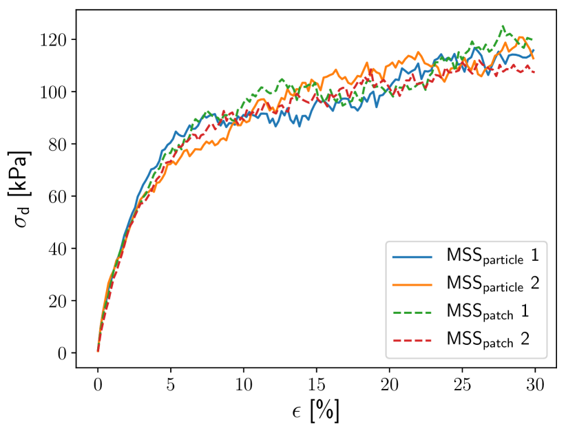
shows the deviatoric stress, $\sigma_{\text{d}}$, as a function of the axial strain, $\epsilon$. The different membrane representations, $\text{MSS}_{\text{particle}}$ and $\text{MSS}_{\text{patch}}$, do not lead to significant differences of the stress-strain behavior.

Table 4 compares the computer time used to simulate a real time of $20\,\text{ms}$.

The reduced number of particles in $\text{MSS}_{\text{patch}}$ accelerates the simulations by about the factor 5, compared to simulations using $\text{MSS}_{\text{particle}}$.

A correct representation of frictional forces at contacts with the membrane is important for many applications. For instance, one of the mechanisms allowing a granular gripper to grasp an object relies on frictional forces brownUniversalRoboticGripper2010 . By construction, an object gliding on a membrane modeled by particles cannot feel a constant (or, at least, smnooth) force.

We demonstrate the smoothness of a membrane modeled by the here described model, and the resulting frictional forces by means of a simple sliding test: In $\text{MSS}_{\text{particle}}$, a membrane is modeled by vertex particles with spacing $1.33\,\text{mm}$. In $\text{MSS}_{\text{patch}}$, the membrane is modeled by patches of side length $1.33\,\text{mm}$.

For the test, we place a spherical particle of radius $2\,\text{mm}$ on a membrane, the free motion of this particle is restricted to the vertical coordinate, perpendicular to the membrane. Its horizontal motion at constant velocity, $0.05\,\text{m/s}$, is enforced externally. Figure 6 shows the particle’s vertical position and the frictional force in sliding direction.

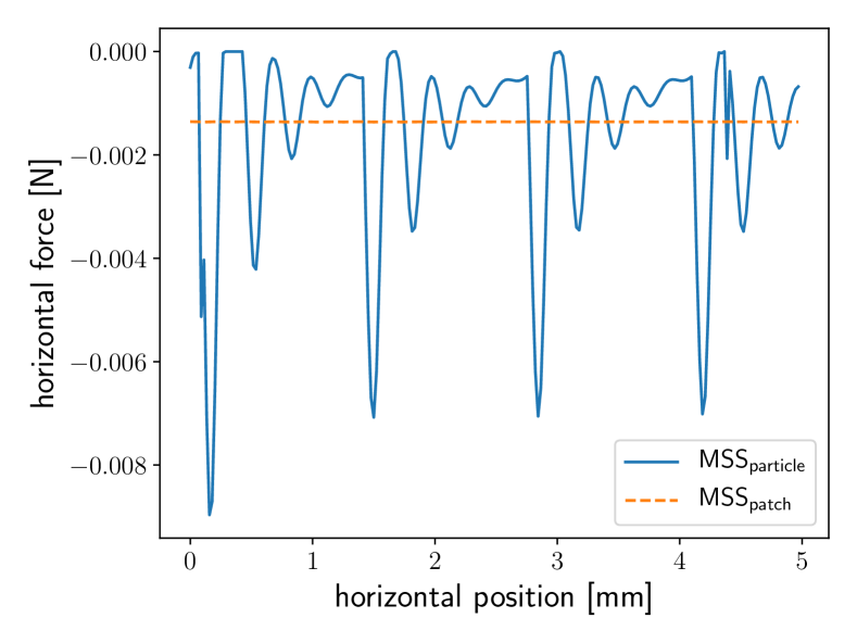
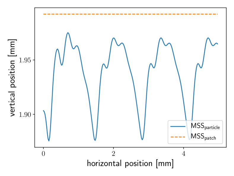
For $\text{MSS}_{\text{particle}}$ we see oscillations in both horizontal force and vertical position. For $\text{MSS}_{\text{patch}}$, we instead observe constant vertical position and constant friction force, as expected when a particle slides on an even plane.

References

- (1) Liu, A. J., Nagel, S. R.: Jamming is not just cool any more. Nature 396, 21–22 (1998). DOI 10.1038/23819
- (2) O’Hern, C. S., Silbert, L. E., Liu, A. J., Nagel, S. R.: Jamming at zero temperature and zero applied stress: The epitome of disorder. Phys. Rev. E 68, 011306 (2003). DOI 10.1103/PhysRevE.68.011306
- (3) Ciamarra, M. P., Nicodemi, M., Coniglio, A.: Recent results on the jamming phase diagram. Soft Matter 6, 2871–2874 (2010). DOI 10.1039/B926810C
- (4) Brown, E., Rodenberg, N., Amend, J., Mozeika, A., Steltz, E., Zakin, M. R., Lipson, H., Jaeger, H. M.: Universal robotic gripper based on the jamming of granular material. PNAS 107, 18809–18814 (2010). DOI 10.1073/pnas.1003250107
- (5) Hauser, S., Eckert, P., Tuleu, A., Ijspeert, A.: Friction and damping of a compliant foot based on granular jamming for legged robots. In: 2016 6th IEEE International Conference on Biomedical Robotics and Biomechatronics (BioRob), pp. 1160–1165 (2016). DOI 10.1109/BIOROB.2016.7523788
- (6) Fitzgerald, S. G., Delaney, G. W., Howard, D.: A Review of jamming actuation in soft robotics. Actuators 9, 104 (2020). DOI 10.3390/act9040104
- (7) de Bono, J., Mcdowell, G., Wanatowski, D.: Discrete element modelling of a flexible membrane for triaxial testing of granular material at high pressures. Geotech. Lett. 2, 199–203 (2012). DOI 10.1680/geolett.12.00040
- (8) Qu, T., Feng, Y. T., Wang, Y., Wang, M.: Discrete element modelling of flexible membrane boundaries for triaxial tests. Comput. Geotech. 115, 103154 (2019). DOI 10.1016/j.compgeo.2019.103154
- (9) Wu, K., Sun, W., Liu, S., Zhang, X.: Study of shear behavior of granular materials by 3D DEM simulation of the triaxial test in the membrane boundary condition. Adv. Powder Technol. 32, 1145–1156 (2021). DOI 10.1016/j.apt.2021.02.018
- (10) Götz, H., Santarossa, A., Sack, A., Pöschel, T., Müller, P.: Soft particles reinforce robotic grippers: Robotic grippers based on granular jamming of soft particles. Granular Matter 24, 31 (2021). DOI 10.1007/s10035-021-01193-4
- (11) Götz, H., Pöschel, T.: Granular meta-material: Viscoelastic response of a bending beam. Granular Matter sumitted (2022)
- (12) Schäfer, J., Dippel, S., Wolf, D. E.: Force schemes in simulations of granular materials. J. Phys. I France 6, 5–20 (1996). DOI 10.1051/jp1:1996129
- (13) Pöschel, T., Schwager, T.: Computational Granular Dynamics: Models and Algorithms. Springer-Verlag, Berlin ; New York (2005)
- (14) Kruggel-Emden, H., Simsek, E., Rickelt, S., Wirtz, S., Scherer, V.: Review and extension of normal force models for the Discrete Element Method. Powder Technology 171, 157–173 (2007). DOI 10.1016/j.powtec.2006.10.004
- (15) Kruggel-Emden, H., Wirtz, S., Scherer, V.: A study on tangential force laws applicable to the discrete element method (DEM) for materials with viscoelastic or plastic behavior. Chemical Engineering Science 63(6), 1523–1541 (2008). DOI 10.1016/j.ces.2007.11.025
- (16) Matuttis, H. G., Chen, J.: Understanding the Discrete Element Method: Simulation of Non-Spherical Particles for Granular and Multi-body Systems. Wiley (2014)
- (17) Kot, M., Nagahashi, H.: Mass spring models with adjustable Poisson’s ratio. Vis. Comput. 33, 283–291 (2017). DOI 10.1007/s00371-015-1194-8
- (18) Ostoja-Starzewski, M.: Lattice models in micromechanics. Appl. Mech. Rev. 55, 35–60 (2002). DOI 10.1115/1.1432990
- (19) Bridson, R., Marino, S., Fedkiw, R.: Simulation of clothing with folds and wrinkles. In: Proceedings of the 2003 ACM SIGGRAPH/Eurographics Symposium on Computer Animation, SCA ’03, pp. 28–36. Eurographics Association, Goslar, DEU (2003)
- (20) Hu, L., Hu, G. M., Fang, Z. Q., Zhang, Y.: A new algorithm for contact detection between spherical particle and triangulated mesh boundary in discrete element method simulations. Int. J. Numer. Methods Eng. 94, 787–804 (2013). DOI 10.1002/nme.4487
- (21) Weinhart, T., Orefice, L., Post, M., van Schrojenstein Lantman, M. P., Denissen, I. F. C., Tunuguntla, D. R., Tsang, J. M. F., Cheng, H., Shaheen, M. Y., Shi, H., Rapino, P., Grannonio, E., Losacco, N., Barbosa, J., Jing, L., Alvarez Naranjo, J. E., Roy, S., den Otter, W. K., Thornton, A. R.: Fast, flexible particle simulations — An introduction to MercuryDPM. Comput. Phys. Commun. 249, 107129 (2020). DOI 10.1016/j.cpc.2019.107129
- (22) Lubachevsky, B. D., Stillinger, F. H.: Geometric properties of random disk packings. J. Stat. Phys. 60, 561–583 (1990). DOI 10.1007/BF01025983