Delay-induced spontaneous dark- state generation from two distant excited atoms

Large-scale interconnected quantum systems offer promising applications in quantum information processing and distributed quantum sensing [1, 2, 3]. As the experimental capabilities for directly interconnecting distant quantum nodes grow [4], we have yet to develop the theoretical toolbox to efficiently analyze systems of multiple qubits collectively exchanging photons over large distances, where delay effects cannot be neglected. Such many-body systems exhibit rich non-Markovian and nonlinear dynamics, arising from delayed and multiphoton interactions. Given the complexity associated with such systems, even the simplest scenarios, e.g., the spontaneous decay of two fully excited distant atoms, remains unexplored.

The most studied cases of coupled emitters consider nearby atoms, neglecting the delay time the field needs to propagate between them. This scenario is a landmark of quantum optics across platforms, such as atoms in free space [5, 6], inside a leaky cavity [7], and near waveguides [8]. In all of these cases, ensembles of initially fully excited two-level atoms decay into their ground state. As atoms decay, correlations among them spontaneously and momentarily emerge, leading to the well-known collective phenomenon of superfluorescence  [9, 10, 11, 6]¹¹1We use the term superfluorescence [9] as a particular case of superradiance when considering a fully inverted sample. Broadly speaking, superradiance is the collective enhancement of the decay rate of an atom in an atomic ensemble beyond the spontaneous emission rate of a single atom [96, 5]. Such atom-atom correlations, which are absent in the initial state, emerge without external driving fields or post-selection  [5].

Platforms based on waveguide QED present an effective way to go beyond the zero-delay approximation, enabling tunable, efficient, and long-ranged interactions in the optical and microwave regime [13, 14, 15, 16, 17, 18, 19, 20, 21]. For example, state-of-the-art experiments allow one to tune out dispersive dipole-dipole interactions by strategically positioning the atoms along a waveguide [22, 23, 24] while highly reducing coupling to non-guided modes [25, 26, 27, 28, 29]. Furthermore, waveguide-coupled quantum emitters enable chiral interactions due to strong spin-momentum coupling, and directional routing of photons [30, 31, 32, 33, 34, 35].

When the time taken by a photon to propagate between two distant emitters becomes comparable to their characteristic lifetimes, the system exhibits surprisingly rich delay-induced non-Markovian dynamics even in the single-photon regime [36, 37, 38, 39, 40, 32]. Some examples of such dynamics include collective spontaneous emission rates exceeding those of Dicke superradiance and formation of highly delocalized atom-photon bound states [41, 42, 43, 44, 45, 46, 47, 48, 49, 50]. In addition, time-delayed feedback can assist in preparing photonic cluster states [51] and single-photon sources with improved coherence and indistinguishability [52].

Recent studies of the effects emerging from delayed interactions considered either many atoms with a single photon [53, 54, 45, 41, 55], many photons with a single atom [44, 56, 57, 58], or numerical exploration of three-photons and three-atoms [50], inviting us to revisit the theoretical description of other canonical quantum optical phenomena, such as superfluorescence, in the context of waveguide-coupled emitters in a large-scale quantum network.

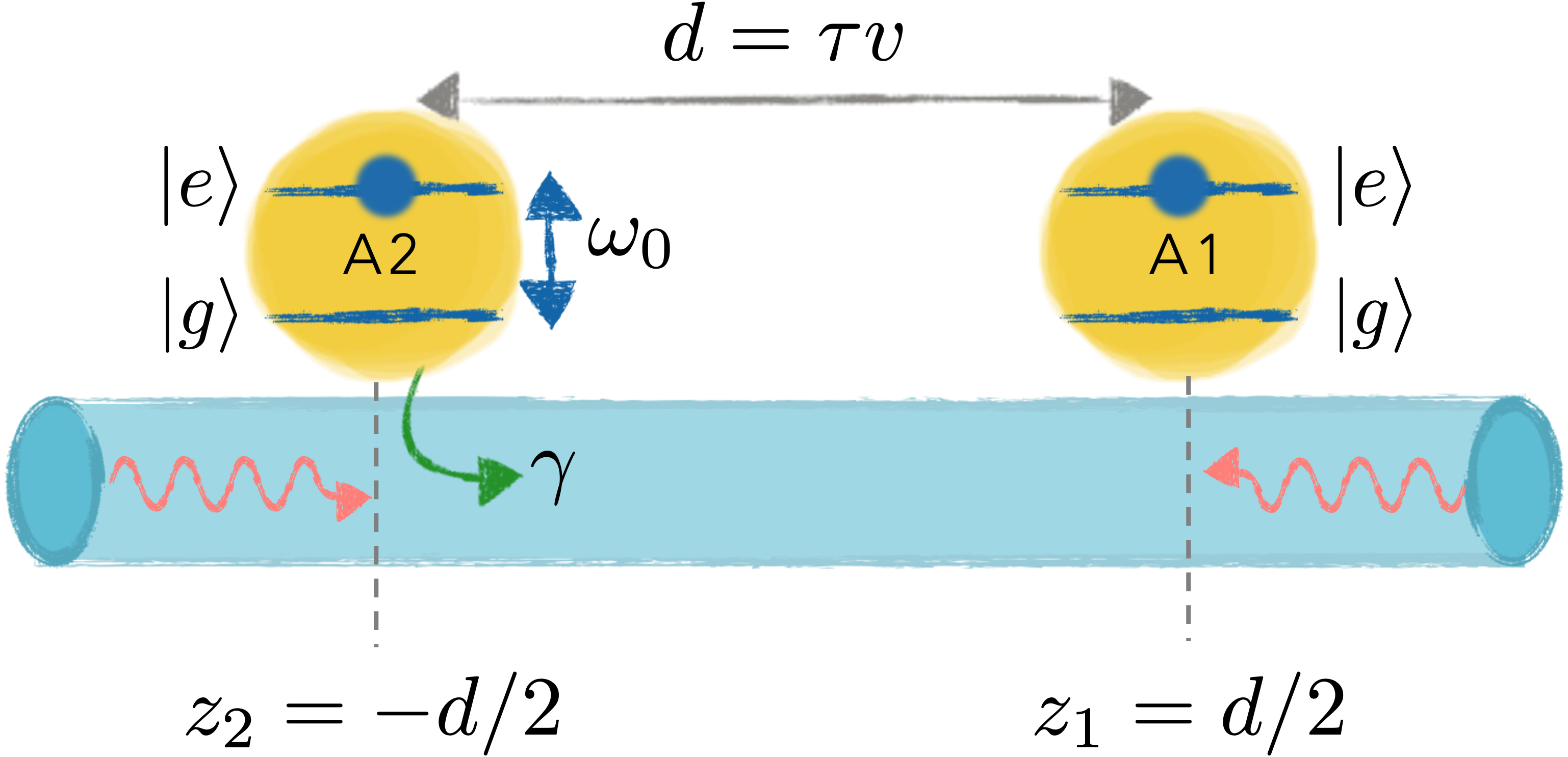
In this paper, we show that a system of two-atoms, with two-excitations, and delayed-interactions (see Fig. 1) exhibits novel non-Markovian collective dynamics. In particular, for fully inverted atoms, the instantaneous decay can be faster than in superfluorescence and steady-state entanglement can suddenly emerge. In the latter case, the electromagnetic (EM) field can have two photons trapped between the two atoms, an effect that can not be captured by Markovian dynamics. We refer to this phenomenon, which leads to the spontaneous generation of a dark state, as delayed-induced subfluorescence –the subradiant counterpart of the well-known superfluorescence effect. The resulting steady state is a delocalized hybrid atom-photon state, requiring a description beyond the usual Born and Markov approximations and qualitatively different from the case without delay, where the system always ends in the ground state. The rich and unique dynamics in such a seemingly simple system demonstrates non-Markovian delay as a mechanism for trapping light, entanglement generation and stabilization in long-distance interacting quantum nodes.

We consider two two-level atoms, with transition frequency $\omega_{0}$ between the ground $\left|g\right\rangle$ and excited $\left|e\right\rangle$ states, coupled through a waveguide. In this work, our emphasis is on the case of perfectly coupled atoms, the free Hamiltonian of the total atoms+field system is given by $H_{0}=(\hbar\omega_{0}/2)\sum_{r=1}^{2}\hat{\sigma}_{z}^{(r)}+\sum_{\alpha,\eta}\hbar\omega_{\alpha}\hat{a}^{\dagger}_{\alpha,\eta}\hat{a}_{\alpha,\eta}$. The interaction Hamiltonian in the interaction picture is (having made the electric-dipole and rotating-wave approximations):

where $g_{\alpha}$ is the coupling between atoms and the guided mode $\alpha$ with frequency $\omega_{\alpha}$, $\Delta_{\alpha}=\omega_{\alpha}-\omega_{0}$, and $k_{\alpha\eta}=\eta\omega_{\alpha}/v$, with $\eta=\pm 1$ specifying the direction of propagation. The position of the atoms is $z_{1,\,2}=\pm d/2$, $\hat{\sigma}_{z}^{(r)}=\left|e\right\rangle_{r}\left\langle e\right|_{r}-\left|g\right\rangle_{r}\left\langle g\right|_{r}$ and the raising and lowering operators for the $r$-th atom are defined as $\hat{\sigma}_{+}^{(r)}=\left(\hat{\sigma}_{-}^{(r)}\right)^{\dagger}=\left|e\right\rangle_{r}\left\langle g\right|_{r}$.

We consider the initial state with both atoms excited and the field in the vacuum state, $\left|e_{1}e_{2},\{0\}\right\rangle$. As a consequence of the rotating-wave approximation, the total number of atomic and field excitations are conserved, suggesting the following ansätz for the state of the system at time $t$:

where $\left|g_{1}g_{2},\{0\}\right\rangle$ is the ground state of the system. The complex coefficients $a(t)$, $b_{\alpha\eta}^{(r)}(t)$, and $c_{\alpha\eta,\beta\eta^{\prime}}(t)$ correspond to the probability amplitudes of having an excitation in both the atoms, $r^{\mathrm{th}}$ atom and field mode $\left\{\alpha,\eta\right\}$, and field modes $\left\{\alpha,\eta\right\}$ and $\left\{\beta,\eta^{\prime}\right\}$, respectively. The coefficients $c_{\alpha\eta}(t)$ represent the probability amplitude of exciting two photons in modes $\left\{\alpha,\eta\right\}$. The Hamiltonian in Eq. (1) models two emitters interacting via the quantized electromagnetic field; their distance, codified in the phase $e^{ik_{\alpha\eta}z_{r}}$, has the effect of introducing a delay in the equations of motion for the quantum state coefficients. This delayed interaction between the emitters results from the finite propagation speed of light.

Defining $B_{\alpha\eta}^{(r)}=b_{\alpha\eta}^{(r)}(t)e^{-i\Delta_{\alpha}t}$ and $C_{\alpha\eta}=c_{\alpha\eta}(t)e^{-2i\Delta_{\alpha}t}$, and formally integrating the equation for $c_{\alpha\eta,\beta\eta^{\prime}}(t)$, the Schrödinger equation yields the following system of delay-differential equations for the excitation amplitudes:

where $\gamma$ is the decay rate of the emitters into the guided modes. We present a detailed derivation in Appendix A. We solve the system of equations via Laplace transforms considering the initial conditions $a(0)=1$ and $B_{\alpha\eta}(0)=C_{\alpha\eta}(0)=0$.

The Laplace transform of $a(t)$ is (see Appendix B)

where $\phi=\omega_{0}\tau$ is the resonance field propagation phase.

We write the sum over modes on the right-hand side (RHS) of Eq. (6) as an integral over frequencies by introducing the density of modes $\rho(\omega_{\alpha})$. Additionally, we use the Wigner-Weisskopf approximation and set $\rho(\omega_{\alpha}),\,g_{\alpha}\approx\rho(\omega_{0}),\,g_{0}$, evaluated at the atomic resonance frequency, a good approximation in the presence of delay effects in waveguide QED [40]. With these considerations we obtain $\tilde{a}(s)=1/(s+\gamma)$ for all $\tau$. Taking the inverse Laplace transform we get $a(t)=e^{-\gamma t}$, which gives the time-dependent probability of having two atomic excitations

We remark that the probability of having two atomic excitations is independent of the delay between atoms.

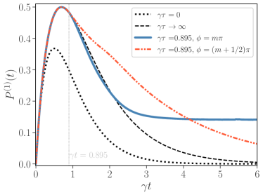
The probability of having only one of the atoms excited is

where the time-dependent solutions $b_{\alpha\eta}^{(1,2)}(t)$ are derived in Appendix B and given by (42). In the limits of two coincident atoms with $\tau=0$, and two infinitely distant atoms with $\tau\to\infty$, we obtain the expected Markovian dynamics [59, 60]:

Figure 2 shows $P^{(1)}(t)$ for different values of the delay $\tau$ and the propagation phase $\phi$. For times $t<\tau$, the atoms decay independently. At time $t=\tau$, the field emitted by one atom reaches the other, modifying their decay dynamics depending on the value of the propagation phase $\phi$. Their instantaneous decay rate, given by the negative slope of $P^{(1)}(t)$, could momentarily exceed that of standard superfluorescence ($\tau=0$). The delay condition $\gamma\tau\approx 0.375$ and $\phi=n\pi$ maximizes the instantaneous decay rate. This phenomenon is a signature of superduperradiance, reported in Ref. [41]. Notably, in this case the atom-atom coherence that is necessary to modify the instantaneous decay emerges spontaneously.

In the late-time limit, the following steady state appears when $\phi=n\pi$ for any delay $\tau$ between the atoms (see Appendix C):

where we have removed the explicit time dependence of the steady-state coefficients. The steady-state amplitude for the mode $\left\{\alpha,\eta\right\}$ is

and $c_{\alpha\eta,\beta\eta^{\prime}}$ is given in Eq. (50)in Appendix C. The last two terms in Eq. (III) represent a bound state in the continuum (BIC) that corresponds to having one shared excitation between the atoms and one propagating photon mode in between them [44]. Using the Born rule and Eq. (11), we obtain that its probability is $2P^{(1)}\left(t\to\infty\right)$, where:

We note that the probability of ending up in a BIC state is maximum for $\gamma\tau\approx 0.895$ with a probability of $0.282$.

The fact that the atoms+field state is non-separable shows that one cannot use the Born-Markov approximation to solve for the dynamics of the system. Using Eq. (III) and Eq. (11) we obtain the following reduced density matrix for the atomic subsystem

with $+$ corresponding to the case when $n$ is odd and $-$ when it is even and $\left|\Psi^{\pm}\right\rangle=(\left|e_{1}g_{2}\right\rangle\pm\left|g_{1}e_{2}\right\rangle)/\sqrt{2}$ are single excitation Bell states. As the initially inverted atoms evolve into a superposition of radiative and non-radiative states upon delayed-interactions, the atoms decay into a superposition of ground state and an entangled dark steady state. For a field propagation phase $\phi=2n\pi$ $(\phi=(2n+1)\pi)$, the dark state that appears in the late-time limit corresponds to the antisymmetric state $\left|\Psi^{-}\right\rangle$ (symmetric state $\left|\Psi^{+}\right\rangle$).

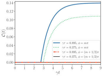
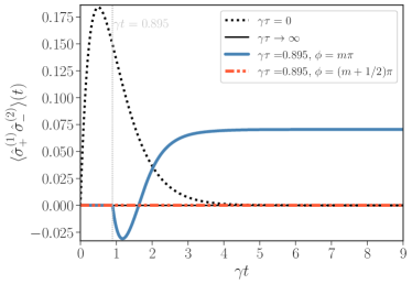
Delayed interactions create quantum correlations between the atoms. We quantify it using the concurrence $\mathcal{C}(t)$ of the reduced density matrix of the atoms $\hat{\rho}_{A}(t)=Tr_{F}(|\psi(t)\rangle\langle\psi(t)\lvert)$ [61]. For $\tau\to\infty$, the concurrence is zero throughout the evolution since the initially uncorrelated atoms evolve independently. Remarkably, when $\tau=0$, the concurrence is also zero throughout the evolution, even when atoms transition to a superradiant behavior. This case exemplifies that entanglement is not necessary for superradiance. For intermediate values of $\tau$, we numerically study the dynamics of concurrence, shown in Fig. 3 (a). We begin studying its behavior for $\gamma\tau\approx 0.895$ (corresponding to the maximum value of $P^{(1)}\left(t\to\infty\right)$) and $\gamma\tau\approx 0.375$ (corresponding to the largest instantaneous decay rate). Since the system lacks initial correlations, the concurrence is zero from $t=0$ to a certain time, $t_{\text{SBE}}$, when there is a sudden birth of entanglement (SBE) [62, 63, 64, 65, 66, 67, 68]. For $\phi=n\pi$, the concurrence increases until reaching a stationary value, whereas for $\phi=(n+\frac{1}{2})\pi$, it always remains zero. In general, for other values of $\phi$, the concurrence suddenly departs from zero and slowly decays after reaching a maximum value. For $\gamma\tau\approx 0.895$, we obtain the maximum value for the concurrence. Figure 3 (b) shows the emergence of atom-atom correlations defined by $\mathrm{Tr}\left[\hat{\rho}_{A}(t)\hat{\sigma}_{+}^{(1)}\hat{\sigma}_{-}^{(2)}\right]$. We note that the atom-atom correlations develop as soon as the atoms “see” each other, while the concurrence takes longer to emerge. Delayed atom-atom interactions couple the fully excited state of the atoms to both single excitation symmetric and antisymmetric states. After the build-up of correlations, the most radiative state collectively decays, while the non-radiative atomic state remains. The system, therefore, spontaneously evolves into an entangled dark state in the presence of retardation. Such appearance of quantum correlations is a striking example of environment-assisted spontaneous entanglement generation.

We now focus on the dynamics of the field sourced by the non-Markovian behavior of the atoms. Field operators are often described through mode expansion, as shown in Eq. (51), or Green’s functions [69]. Its expectation values involve integrating over all the modes or knowing the Green’s function for the field, which for waveguides is usually given by a mode expansion [70]. When the system is Markovian, an input-output relation simplifies the calculation of field observables, and the sum over field modes is replaced by a sum over atomic operators: $\hat{{\mathbf{E}}}^{+}({\mathbf{r}})={\hat{{\mathbf{E}}}}^{+}_{\textrm{Input}}({\mathbf{r}})+\sum_{i}f({\mathbf{r}},{\mathbf{r}_{i}})\hat{\sigma}_{-}^{i}$, where the positive part of the field operator, $\hat{{\mathbf{E}}}^{+}({\mathbf{r}})$, at ${\mathbf{r}}$, is proportional to the input field, $\hat{{\mathbf{E}}}^{+}_{\textrm{Input}}({\mathbf{r}})$, plus the field sourced by the atomic operators $\hat{\sigma}_{-}^{i}$. Here ${\mathbf{r}_{i}}$ is the position of atom $i$, and $f({\mathbf{r}},{\mathbf{r}_{i}})$ is a complex function that depends on the modes of the system [14, 71].

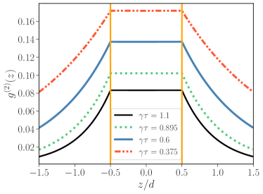
The probability of measuring two photons at the same time at position $z$ is proportional to the second-order correlation function [72]

where we take the maximum over the distance between the atoms, in the normalization constant, to compare the second-order correlation function for different time lags. By substituting the input-output relation for the Markovian case into $g^{(2)}$ and replacing it with the stationary solution, Eq. (III), we see that the dynamics does not lead to a two-photon bound state. However, the system under consideration is non-Markovian, and one must calculate the field observables from the full expression for the field operator.

Figure  4 shows the second-order correlation function in the stationary regime ($t\to\infty$) (see Appendix D for details), for different distances between the atoms. It can be seen that two photons are trapped between the atoms, a result that is distinctly non-Markovian, demonstrating the rich interplay of non-Markovianity and nonlinear atom-photon interactions. Although the maximum probability of having the atoms excited is given at a distance $\gamma\tau\approx 0.895$, the probability of having two photons excited at a particular $z$ is greater at $\gamma\tau\approx 0.375$, where the instantaneous decay is maximum. This is explained by the fact that the probability of having two photons trapped in a particular position increases when the probability of the atomic excitation diminishes, because the energy from the atomic excitation should go to the field.

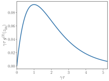
A salient question pertains to the maximum probability of having two photons between the atoms. This probability depends on the value of the autocorrelation function and the distance between the two atoms. Figure 5 depicts $\gamma\tau\,g^{(2)}(z_{\textrm{in}})$, which is proportional to the probability of having two photons in the waveguide region separating the two atoms as a function of the delay. The distance between the atoms where the probability of having two photons is maximum is $\gamma\tau\approx 1.0$.

Note that we chose a normalization that does not depend on the transverse profile (see Appendix D for details). To obtain the actual probability that two photon detection happen at the same time and position, it is useful to calculate the field energy in the guided field modes, in the limit $t\to\infty$ (see Appendix C)

where $P^{(1)}\left(t\to\infty\right)$ is the probability of having one atomic excitation in the long time limit (see Eq. (12)). This result states that the total field energy corresponds to the energy of two photons with frequency $\omega_{0}$ (the total energy) minus the energy accumulated in the atoms that has not been emitted into the waveguide. The normalization constant, $\int dz\langle\hat{{\mathbf{E}}}^{(+)}(z)\hat{{\mathbf{E}}}^{(-)}(z)\rangle$, is given by the total energy around the fiber, $\mathcal{E}_{\textrm{total}}$ (see Eq. (15)) multiplied by the square of the mode profile at the atomic frequency transition $\omega_{0}$.

We have analyzed the spontaneous decay of two fully inverted atoms coupled through a waveguide in the presence of retardation effects. A remarkable result is the spontaneous creation of a steady delocalized atom-photon bound state, with sudden birth of entanglement between the atoms. Furthermore, we demonstrate that such a delay can create two-photon bound states, wherein one can have two photons in the waveguide region between the two atoms. Such states appear as a result of the non-Markovian time-delayed feedback of the spontaneously radiated EM field acting on the emitters. Additionally, the collective decay of the two atoms can be momentarily enhanced beyond standard superfluorescence and subsequently inhibited, demonstrating the rich non-Markovian dynamics of such a system.

Such delay-induced spontaneous steady state entanglement generation can have implications in the rapidly growing field of waveguide QED, a field with promising applications in quantum information processing [73, 3, 74, 75, 76, 77, 78, 79] that benefit from preparing and manipulating long-lived dark-states. In this context, there have been several proposals to generate a steady entangled state; compared to delay-induced subfluorescence, these schemes necessitate extra degrees of control, such as external driving fields [80, 81, 82, 36], initial entanglement [41], or chiral emission in front of a mirror [39, 83].

It is not only the generation [84] but also the stabilization of entangled states that are critical to developing efficient quantum devices. In contrast to the idea that the interaction of quantum systems with their environment leads to decoherence and can degrade the entanglement between the components of a quantum system [85], the environment can also be proposed as a generator [86, 87] and stabilizer of entanglement [88]. Our results demonstrate that non-Markovian time-delayed feedback can be a mechanism for environment-assisted entanglement generation and stabilization.

Adding delay to the most straightforward collective system of two two-level atoms leads to different phenomenology, breaking the Born and Markov approximations, non-trivially modifying the dynamics, and spontaneously creating steady-state quantum correlations between the atoms and multiphoton bound states. Our results further the understanding of the significant role delay plays in quantum optics and present the outset of studying more complex phenomena involving many-body interactions [6, 89, 90]. However, studying this scenario is challenging as the complexity of the problem increases with the number of emitters, and known methods based on master equation approaches fail because neither the Markov nor the Born approximations are valid. Furthermore, although we neglect dispersive dipole-dipole interactions and coupling to non-guided modes to highlight the consequences of delay-induced non-Markovianity, all these effects can coexist, creating richer dynamics that will increase in complexity as the system scales up.

We acknowledge helpful discussions with Saikat Guha and Elizabeth Goldschmidt. P.S. is a CIFAR Azrieli Global Scholar in the Quantum Information Science Program. This work was supported by DGAPA-UNAM under grant IG101421 and IG101324 from Mexico, as well as CONICYT-PAI grant 77190033, and FONDECYT grant N^∘ 11200192 from Chile. K.S. acknowledges funding support from the John Templeton Foundation Award No. 62422, the National Science Foundation under Grant No. PHY-2309341 and the Army Research Office through Grant No. W911NF2410080.

References

- Kimble [2008] H. J. Kimble, The quantum internet, Nature 453, 1023 (2008).
- Duan and Monroe [2010] L.-M. Duan and C. Monroe, Colloquium: Quantum networks with trapped ions, Rev. Mod. Phys. 82, 1209 (2010).
- Monroe et al. [2014] C. Monroe, R. Raussendorf, A. Ruthven, K. R. Brown, P. Maunz, L.-M. Duan, and J. Kim, Large-scale modular quantum-computer architecture with atomic memory and photonic interconnects, Phys. Rev. A 89, 022317 (2014).
- Storz et al. [2023] S. Storz, J. Schär, A. Kulikov, P. Magnard, P. Kurpiers, J. Lütolf, T. Walter, A. Copetudo, K. Reuer, A. Akin, J.-C. Besse, M. Gabureac, G. J. Norris, A. Rosario, F. Martin, J. Martinez, W. Amaya, M. W. Mitchell, C. Abellan, J.-D. Bancal, N. Sangouard, B. Royer, A. Blais, and A. Wallraff, Loophole-free bell inequality violation with superconducting circuits, Nature 617, 265 (2023).
- Gross and Haroche [1982] M. Gross and S. Haroche, Superradiance: An essay on the theory of collective spontaneous emission, Physics Reports 93, 301 (1982).
- Clemens et al. [2003] J. P. Clemens, L. Horvath, B. C. Sanders, and H. J. Carmichael, Collective spontaneous emission from a line of atoms, Phys. Rev. A 68, 023809 (2003).
- Clemens and Carmichael [2002] J. P. Clemens and H. J. Carmichael, Stochastic initiation of superradiance in a cavity: An approximation scheme within quantum trajectory theory, Phys. Rev. A 65, 023815 (2002).
- Le Kien et al. [2005] F. Le Kien, S. D. Gupta, K. P. Nayak, and K. Hakuta, Nanofiber-mediated radiative transfer between two distant atoms, Phys. Rev. A 72, 063815 (2005).
- Bonifacio and Lugiato [1975] R. Bonifacio and L. A. Lugiato, Cooperative radiation processes in two-level systems: Superfluorescence, Phys. Rev. A 11, 1507 (1975).
- Glauber and Haake [1978] R. Glauber and F. Haake, The initiation of superfluorescence, Physics Letters A 68, 29 (1978).
- Vrehen et al. [1980] Q. Vrehen, M. Schuurmans, and D. Polder, Superfluorescence: macroscopic quantum fluctuations in the time domain, Nature 285, 70 (1980).
- Note [1] We use the term superfluorescence [9] as a particular case of superradiance when considering a fully inverted sample. Broadly speaking, superradiance is the collective enhancement of the decay rate of an atom in an atomic ensemble beyond the spontaneous emission rate of a single atom [96, 5].
- Goban et al. [2015] A. Goban, C.-L. Hung, J. D. Hood, S.-P. Yu, J. A. Muniz, O. Painter, and H. J. Kimble, Superradiance for atoms trapped along a photonic crystal waveguide, Phys. Rev. Lett. 115, 063601 (2015).
- Solano et al. [2017a] P. Solano, P. Barberis-Blostein, F. K. Fatemi, L. A. Orozco, and S. L. Rolston, Super-radiance reveals infinite-range dipole interactions through a nanofiber, Nat. Commun. 8, 1857 (2017a).
- Solano et al. [2017b] P. Solano, J. A. Grover, J. E. Hoffman, S. Ravets, F. K. Fatemi, L. A. Orozco, S. L. Rolston, and A. Optical Nanofibers:, New platform for quantum optics, Adv. At. Mol. Opt. Phys. 66, 439 (2017b).
- Kim et al. [2018] J.-H. Kim, S. Aghaeimeibodi, C. J. K. Richardson, R. P. Leavitt, and E. Waks, Super-radiant emission from quantum dots in a nanophotonic waveguide, Nano Letters 18, 4734 (2018).
- Wen et al. [2019] P. Y. Wen, K.-T. Lin, A. F. Kockum, B. Suri, H. Ian, J. C. Chen, S. Y. Mao, C. C. Chiu, P. Delsing, F. Nori, G.-D. Lin, and I.-C. Hoi, Large collective lamb shift of two distant superconducting artificial atoms, Phys. Rev. Lett 123, 233602 (2019).
- Mirhosseini et al. [2019] M. Mirhosseini, E. Kim, X. Zhang, A. Sipahigil, P. B. Dieterle, A. J. Keller, A. Asenjo-Garcia, D. E. Chang, and O. Painter, Cavity quantum electrodynamics with atom-like mirrors, Nature 569, 692 (2019).
- Sheremet et al. [2023] A. S. Sheremet, M. I. Petrov, I. V. Iorsh, A. V. Poshakinskiy, and A. N. Poddubny, Waveguide quantum electrodynamics: Collective radiance and photon-photon correlations, Rev. Mod. Phys. 95, 015002 (2023).
- Magnard et al. [2020] P. Magnard, S. Storz, P. Kurpiers, J. Schär, F. Marxer, J. Lütolf, T. Walter, J.-C. Besse, M. Gabureac, K. Reuer, A. Akin, B. Royer, A. Blais, and A. Wallraff, Microwave quantum link between superconducting circuits housed in spatially separated cryogenic systems, Phys. Rev. Lett. 125, 260502 (2020).
- Tiranov et al. [2023] A. Tiranov, V. Angelopoulou, C. J. van Diepen, B. Schrinski, O. A. D. Sandberg, Y. Wang, L. Midolo, S. Scholz, A. D. Wieck, A. Ludwig, A. S. Sørensen, and P. Lodahl, Collective super- and subradiant dynamics between distant optical quantum emitters, Science 379, 389 (2023).
- Martín-Cano et al. [2011] D. Martín-Cano, A. González-Tudela, L. Martín-Moreno, F. J. García-Vidal, C. Tejedor, and E. Moreno, Dissipation-driven generation of two-qubit entanglement mediated by plasmonic waveguides, Phys. Rev. B 84, 235306 (2011).
- van Loo et al. [2013] A. F. van Loo, A. Fedorov, K. Lalumière, B. C. Sanders, A. Blais, and A. Wallraff, Photon-mediated interactions between distant artificial atoms, Science 342, 1494 (2013).
- Pichler et al. [2015] H. Pichler, T. Ramos, A. J. Daley, and P. Zoller, Quantum optics of chiral spin networks, Phys. Rev. A 91, 042116 (2015).
- Lecamp et al. [2007] G. Lecamp, P. Lalanne, and J. P. Hugonin, Very large spontaneous-emission factors in photonic-crystal waveguides, Phys. Rev. Lett. 99, 023902 (2007).
- Astafiev et al. [2010] O. Astafiev, A. M. Zagoskin, A. Abdumalikov Jr, Y. A. Pashkin, T. Yamamoto, K. Inomata, Y. Nakamura, and J. S. Tsai, Resonance fluorescence of a single artificial atom, Science 327, 840 (2010).
- Arcari et al. [2014] M. Arcari, I. Söllner, A. Javadi, S. Lindskov Hansen, S. Mahmoodian, J. Liu, H. Thyrrestrup, E. H. Lee, J. D. Song, S. Stobbe, and P. Lodahl, Near-unity coupling efficiency of a quantum emitter to a photonic crystal waveguide, Phys. Rev. Lett. 113, 093603 (2014).
- Zang et al. [2016] X. Zang, J. Yang, R. Faggiani, C. Gill, P. G. Petrov, J.-P. Hugonin, K. Vynck, S. Bernon, P. Bouyer, V. Boyer, and P. Lalanne, Interaction between atoms and slow light: A study in waveguide design, Phys. Rev. Appl. 5, 024003 (2016).
- Scarpelli et al. [2019] L. Scarpelli, B. Lang, F. Masia, D. M. Beggs, E. A. Muljarov, A. B. Young, R. Oulton, M. Kamp, S. Höfling, C. Schneider, and W. Langbein, 99directional coupling of quantum dots to fast light in photonic crystal waveguides determined by spectral imaging, Phys. Rev. B 100, 035311 (2019).
- Lodahl et al. [2017] P. Lodahl, S. Mahmoodian, S. Stobbe, A. Rauschenbeutel, P. Schneeweiss, J. Volz, H. Pichler, and P. Zoller, Chiral quantum optics, Nature 541, 473 (2017).
- Kannan et al. [2023] B. Kannan, A. Almanakly, Y. Sung, A. Di Paolo, D. A. Rower, J. Braumüller, A. Melville, B. M. Niedzielski, A. Karamlou, K. Serniak, A. Vepsäläinen, M. E. Schwartz, J. L. Yoder, R. Winik, J. I.-J. Wang, T. P. Orlando, S. Gustavsson, J. A. Grover, and W. D. Oliver, On-demand directional microwave photon emission using waveguide quantum electrodynamics, Nature Physics 19, 394 (2023).
- Solano et al. [2023] P. Solano, P. Barberis-Blostein, and K. Sinha, Dissimilar collective decay and directional emission from two quantum emitters, Phys. Rev. A 107, 023723 (2023).
- Maffei et al. [2024] M. Maffei, D. Pomarico, P. Facchi, G. Magnifico, S. Pascazio, and F. Pepe, Directional emission and photon bunching from a qubit pair in waveguide (2024), arXiv:2402.01286 [quant-ph] .
- Lin et al. [2019] W. Lin, Y. Ota, S. Iwamoto, and Y. Arakawa, Spin-dependent directional emission from a quantum dot ensemble embedded in an asymmetric waveguide, Opt. Lett. 44, 3749 (2019).
- Petersen et al. [2014] J. Petersen, J. Volz, and A. Rauschenbeutel, Chiral nanophotonic waveguide interface based on spin-orbit interaction of light, Science 346, 67 (2014).
- Zheng and Baranger [2013] H. Zheng and H. U. Baranger, Persistent quantum beats and long-distance entanglement from waveguide-mediated interactions, Phys. Rev. Lett. 110, 113601 (2013).
- Tufarelli et al. [2014] T. Tufarelli, M. S. Kim, and F. Ciccarello, Non-markovianity of a quantum emitter in front of a mirror, Phys. Rev. A 90, 012113 (2014).
- Guimond et al. [2016] P.-O. Guimond, A. Roulet, H. N. Le, and V. Scarani, Rabi oscillation in a quantum cavity: Markovian and non-markovian dynamics, Phys. Rev. A 93, 023808 (2016).
- Zhang et al. [2020] B. Zhang, S. You, and M. Lu, Enhancement of spontaneous entanglement generation via coherent quantum feedback, Phys. Rev. A 101, 032335 (2020).
- Del Ángel et al. [2022] A. Del Ángel, P. Solano, and P. Barberis-Blostein, Effects of environment correlations on the onset of collective decay in waveguide qed, arXiv:2212.01972 (2022).
- Sinha et al. [2020a] K. Sinha, P. Meystre, E. A. Goldschmidt, F. K. Fatemi, S. L. Rolston, and P. Solano, Non-markovian collective emission from macroscopically separated emitters, Phys. Rev. Lett. 124, 043603 (2020a).
- Sinha et al. [2020b] K. Sinha, A. González-Tudela, Y. Lu, and P. Solano, Collective radiation from distant emitters, Phys. Rev. A 102, 043718 (2020b).
- Dinç and Brańczyk [2019] F. Dinç and A. M. Brańczyk, Non-markovian super-superradiance in a linear chain of up to 100 qubits, Phys. Rev. Research 1, 032042(R) (2019).
- Calajó et al. [2019] G. Calajó, Y.-L. L. Fang, H. U. Baranger, and F. Ciccarello, Exciting a bound state in the continuum through multiphoton scattering plus delayed quantum feedback, Phys. Rev. Lett. 122, 073601 (2019).
- Facchi et al. [2019] P. Facchi, D. Lonigro, S. Pascazio, F. V. Pepe, and D. Pomarico, Bound states in the continuum for an array of quantum emitters, Phys. Rev. A 100, 023834 (2019).
- Guo et al. [2020] L. Guo, A. F. Kockum, F. Marquardt, and G. Johansson, Oscillating bound states for a giant atom, Phys. Rev. Research 2, 043014 (2020).
- Yao and Hughes [2009] P. Yao and S. Hughes, Macroscopic entanglement and violation of bell’s inequalities between two spatially separated quantum dots in a planar photonic crystal system, Opt. Express 17, 11505 (2009).
- Crowder et al. [2020] G. Crowder, H. Carmichael, and S. Hughes, Quantum trajectory theory of few-photon cavity-qed systems with a time-delayed coherent feedback, Phys. Rev. A 101, 023807 (2020).
- Lee et al. [2023] A. Lee, H. S. Han, F. K. Fatemi, S. L. Rolston, and K. Sinha, Collective quantum beats from distant multilevel emitters, Phys. Rev. A 107, 013701 (2023).
- Carmele et al. [2020] A. Carmele, N. Nemet, V. Canela, and S. Parkins, Pronounced non-markovian features in multiply excited, multiple emitter waveguide qed: Retardation induced anomalous population trapping, Phys. Rev. Res. 2, 013238 (2020).
- Pichler et al. [2017] H. Pichler, S. Choi, P. Zoller, and M. D. Lukin, Universal photonic quantum computation via time-delayed feedback, Proceedings of the National Academy of Sciences 114, 11362 (2017).
- Crowder et al. [2023] G. Crowder, L. Ramunno, and S. Hughes, Improving on-demand single photon source coherence and indistinguishability through a time-delayed coherent feedback, arXiv:2302.08093 (2023).
- Gonzalez-Ballestero et al. [2013] C. Gonzalez-Ballestero, F. J. García-Vidal, and E. Moreno, Non-markovian effects in waveguide-mediated entanglement, New Journal of Physics 15, 073015 (2013).
- Liao et al. [2015] Z. Liao, X. Zeng, S.-Y. Zhu, and M. S. Zubairy, Single-photon transport through an atomic chain coupled to a one-dimensional nanophotonic waveguide, Phys. Rev. A 92, 023806 (2015).
- Pivovarov et al. [2021] V. A. Pivovarov, L. V. Gerasimov, J. Berroir, T. Ray, J. Laurat, A. Urvoy, and D. V. Kupriyanov, Single collective excitation of an atomic array trapped along a waveguide: A study of cooperative emission for different atomic chain configurations, Phys. Rev. A 103, 043716 (2021).
- Guo et al. [2017] L. Guo, A. Grimsmo, A. F. Kockum, M. Pletyukhov, and G. Johansson, Giant acoustic atom: A single quantum system with a deterministic time delay, Phys. Rev. A 95, 053821 (2017).
- Guimond et al. [2017] P.-O. Guimond, M. Pletyukhov, H. Pichler, and P. Zoller, Delayed coherent quantum feedback from a scattering theory and a matrix product state perspective, Quantum Science and Technology 2, 044012 (2017).
- Fang et al. [2018] Y.-L. L. Fang, F. Ciccarello, and H. U. Baranger, Non-markovian dynamics of a qubit due to single-photon scattering in a waveguide, New Journal of Physics 20, 043035 (2018).
- Lehmberg [1970] R. H. Lehmberg, Radiation from an -atom system. ii. spontaneous emission from a pair of atoms, Phys. Rev. A 2, 889 (1970).
- Alvarez-Giron and Barberis-Blostein [2020] W. Alvarez-Giron and P. Barberis-Blostein, The atomic damping basis and the collective decay of interacting two-level atoms, Journal of Physics A: Mathematical and Theoretical 53, 435301 (2020).
- Wootters [1998] W. K. Wootters, Entanglement of formation of an arbitrary state of two qubits, Phys. Rev. Lett. 80, 2245 (1998).
- López et al. [2008] C. E. López, G. Romero, F. Lastra, E. Solano, and J. C. Retamal, Sudden birth versus sudden death of entanglement in multipartite systems, Phys. Rev. Lett. 101, 080503 (2008).
- Mazzola et al. [2009] L. Mazzola, S. Maniscalco, J. Piilo, K.-A. Suominen, and B. M. Garraway, Sudden death and sudden birth of entanglement in common structured reservoirs, Phys. Rev. A 79, 042302 (2009).
- Ficek and Tanaś [2003] Z. Ficek and R. Tanaś, Entanglement induced by spontaneous emission in spatially extended two-atom systems, Journal of Modern Optics 50, 2765 (2003).
- Tanaś and Ficek [2004] R. Tanaś and Z. Ficek, Entangling two atoms via spontaneous emission, Journal of Optics B: Quantum and Semiclassical Optics 6, S90 (2004).
- Ficek and Tanaś [2007] Z. Ficek and R. Tanaś, Spontaneously induced sudden birth of entanglement, in Quantum-Atom Optics Downunder (Optica Publishing Group, 2007) p. QME11.
- Ficek and Tanaś [2008] Z. Ficek and R. Tanaś, Delayed sudden birth of entanglement, Phys. Rev. A 77, 054301 (2008).
- Ashrafi and Naderi [2013] M. Ashrafi and M. Naderi, Entanglement sudden birth and sudden death in a system of two distant atoms coupled via an optical element, Journal of Modern Optics 60, 331 (2013).
- Gruner and Welsch [1996] T. Gruner and D.-G. Welsch, Green-function approach to the radiation-field quantization for homogeneous and inhomogeneous kramers-kronig dielectrics, Phys. Rev. A 53, 1818 (1996).
- Asenjo-Garcia et al. [2017] A. Asenjo-Garcia, M. Moreno-Cardoner, A. Albrecht, H. J. Kimble, and D. E. Chang, Exponential improvement in photon storage fidelities using subradiance and “selective radiance” in atomic arrays, Phys. Rev. X 7, 031024 (2017).
- Chang et al. [2012] D. E. Chang, L. Jiang, A. V. Gorshkov, and H. J. Kimble, Cavity qed with atomic mirrors, New Journal of Physics 14, 063003 (2012).
- Glauber [1963] R. J. Glauber, The quantum theory of optical coherence, Phys. Rev. 130, 2529 (1963).
- Zheng et al. [2013] H. Zheng, D. J. Gauthier, and H. U. Baranger, Waveguide-qed-based photonic quantum computation, Phys. Rev. Lett. 111, 090502 (2013).
- Javadi et al. [2015] A. Javadi, I. Söllner, M. Arcari, S. L. Hansen, L. Midolo, S. Mahmoodian, G. Kiršanskė, T. Pregnolato, E. H. Lee, J. D. Song, S. Stobbe, and P. Lodahl, Single-photon non-linear optics with a quantum dot in a waveguide, Nature Communications 6, 8655 (2015).
- Tian et al. [2021] Z. Tian, P. Zhang, and X.-W. Chen, Static hybrid quantum nodes: Toward perfect state transfer on a photonic chip, Phys. Rev. Appl. 15, 054043 (2021).
- Yan et al. [2015] W.-B. Yan, B. Liu, L. Zhou, and H. Fan, All-optical router at single-photon level by interference, Europhysics Letters 111, 64005 (2015).
- Coles et al. [2016] R. J. Coles, D. M. Price, J. E. Dixon, B. Royall, E. Clarke, P. Kok, M. S. Skolnick, A. M. Fox, and M. N. Makhonin, Chirality of nanophotonic waveguide with embedded quantum emitter for unidirectional spin transfer, Nature Communications 7, 11183 (2016).
- Chang et al. [2020] H.-S. Chang, Y. P. Zhong, A. Bienfait, M.-H. Chou, C. R. Conner, E. Dumur, J. Grebel, G. A. Peairs, R. G. Povey, K. J. Satzinger, and A. N. Cleland, Remote entanglement via adiabatic passage using a tunably dissipative quantum communication system, Phys. Rev. Lett. 124, 240502 (2020).
- Zhong et al. [2021] Y. Zhong, H.-S. Chang, A. Bienfait, É. Dumur, M.-H. Chou, C. R. Conner, J. Grebel, R. G. Povey, H. Yan, D. I. Schuster, and A. N. Cleland, Deterministic multi-qubit entanglement in a quantum network, Nature 590, 571 (2021).
- Paulisch et al. [2016] V. Paulisch, H. J. Kimble, and A. González-Tudela, Universal quantum computation in waveguide qed using decoherence free subspaces, New Journal of Physics 18, 043041 (2016).
- Zanner et al. [2022] M. Zanner, T. Orell, C. M. F. Schneider, R. Albert, S. Oleschko, M. L. Juan, M. Silveri, and G. Kirchmair, Coherent control of a multi-qubit dark state in waveguide quantum electrodynamics, Nature Physics 18, 538 (2022).
- Gonzalez-Tudela et al. [2011] A. Gonzalez-Tudela, D. Martin-Cano, E. Moreno, L. Martin-Moreno, C. Tejedor, and F. J. Garcia-Vidal, Entanglement of two qubits mediated by one-dimensional plasmonic waveguides, Phys. Rev. Lett. 106, 020501 (2011).
- Ask and Johansson [2022] A. Ask and G. Johansson, Non-markovian steady states of a driven two-level system, Phys. Rev. Lett. 128, 083603 (2022).
- Horodecki et al. [2009] R. Horodecki, P. Horodecki, M. Horodecki, and K. Horodecki, Quantum entanglement, Rev. Mod. Phys. 81, 865 (2009).
- Plenio and Knight [1998] M. B. Plenio and P. L. Knight, The quantum-jump approach to dissipative dynamics in quantum optics, Rev. Mod. Phys. 70, 101 (1998).
- Kraus et al. [2008] B. Kraus, H. P. Büchler, S. Diehl, A. Kantian, A. Micheli, and P. Zoller, Preparation of entangled states by quantum markov processes, Phys. Rev. A 78, 042307 (2008).
- Verstraete et al. [2009] F. Verstraete, M. M. Wolf, and J. Ignacio Cirac, Quantum computation and quantum-state engineering driven by dissipation, Nature Physics 5, 633 (2009).
- Tacchino et al. [2018] F. Tacchino, A. Auffèves, M. F. Santos, and D. Gerace, Steady state entanglement beyond thermal limits, Phys. Rev. Lett. 120, 063604 (2018).
- Masson and Asenjo-Garcia [2022] S. J. Masson and A. Asenjo-Garcia, Universality of dicke superradiance in arrays of quantum emitters, Nature Communications 13, 1 (2022).
- Masson et al. [2020] S. J. Masson, I. Ferrier-Barbut, L. A. Orozco, A. Browaeys, and A. Asenjo-Garcia, Many-body signatures of collective decay in atomic chains, Phys. Rev. Lett. 125, 263601 (2020).
- Loudon [1983] R. Loudon, The Quantum Theory of Light, 2nd ed. (Clarendon Press, Oxford, 1983).
- Barnes et al. [2020] W. L. Barnes, S. A. R. Horsley, and W. L. Vos, Classical antennas, quantum emitters, and densities of optical states, Journal of Optics 22, 073501 (2020).
- Corless et al. [1996] R. M. Corless, G. H. Gonnet, D. E. G. Hare, D. J. Jeffrey, and D. E. Knuth, On the lambertw function, Advances in Computational Mathematics 5, 329 (1996).
- Rao and Ahmed [1968] K. R. Rao and N. Ahmed, Recursive techniques for obtaining the partial fraction expansion of a rational function, IEEE Transactions on Education 11, 152 (1968).
- Cohen [2020] H. Cohen, Lambert -function branch identities, arXiv:2012.11698 (2020).
- Dicke [1954] R. H. Dicke, Coherence in spontaneous radiation processes, Phys. Rev. 93, 99 (1954).