Degree-degree Correlated Low-density Parity-check Codes Over a Binary Erasure Channel
Abstract
Most existing works on analyzing the performance of a random ensemble of low-density parity-check (LDPC) codes assume that the degree distributions of the two ends of a randomly selected edge are independent. In the paper, we take one step further and consider ensembles of LDPC codes with degree-degree correlations. For this, we propose two methods to construct an ensemble of degree-degree correlated LDPC codes. We then derive a system of density evolution equations for such degree-degree correlated LDPC codes over a binary erasure channel (BEC). By conducting extensive numerical experiments, we show how the degree-degree correlation affects the performance of LDPC codes. Our numerical results show that LDPC codes with negative degree-degree correlation could improve the maximum tolerable erasure probability. Moreover, increasing the negative degree-degree correlation could lead to better unequal error protection (UEP) design.
I Introduction
Low-density parity-check (LDPC) codes, first introduced by R. Gallager in 1962 [1], have been widely used in practice, including the 5G new radio wireless communication standard (see, e.g., [2, 3]) and the flash-memory systems (see, e.g., [4, 5]). LDPC codes are linear block codes that can be characterized by either a generator matrix or a parity-check matrix. It is well-known that there is a one-to-one mapping between the generator matrix and the parity-check matrix (see, e.g., Section II.B of the survey paper [6]). In particular, for an -LDPC code, there are information bits in a codeword of bits. The generator matrix then maps the information bits to the codeword bits by multiplying the vector of the information bits with the generator matrix. On the other hand, the parity-check matrix can be used for checking whether an -bit binary vector is a legitimate codeword and decoding the information bits from that codeword.
The parity-check matrix associated with an -LDPC code can be represented by a bipartite graph, commonly known as the Tanner graph [7]. For such a bipartite graph, there are variable nodes on one side and check nodes on the other side. A check node represents a constraint on the values of variable nodes connected to that check node. In particular, for binary-valued variables, the value of a check node is simply the checksum of the values of the variable nodes connected to that check node. For a legitimate codeword, the checksums of the check nodes are all 0’s. In other words, multiplying a codeword with the parity-check matrix yields a vector with all 0’s.
Performance analysis of LDPC codes over a binary erasure channel (BEC) has been studied extensively in the literature (see e.g., [8, 9, 10, 11]). For a BEC with the erasure probability , each bit in a codeword is erased independently with probability . To recover the erased code bits, one can apply an iterative decoding (peeling) algorithm described below. First, the values of the non-erased variable nodes are added to the check nodes connected to them. Subsequently, these non-erased nodes and their edges are removed. The remaining bipartite graph consists only of erased variable nodes. An erased variable node connected to a check node with degree 1 can be decoded by the value of that check node. Upon successful decoding, the erased variable node becomes a non-erased node and can be removed similarly to the original non-erased nodes. Repeat this process until no more erased variable nodes can be decoded.
A probabilistic framework for analyzing the iterative algorithm is known as the density evolution method [9, 10, 11]. Such a method tracks the probability that the variable end of a randomly selected edge is not decoded after each iteration. The evolution of such a probability is characterized by the degree distribution of a randomly selected variable node and that of a randomly selected check node. The density evolution method can also be extended to provide unequal error protection of code bits [12, 13, 14, 15, 16]. For the setting with unequal error protection, code bits are classified into several classes, and the density evolution method tracks the probability that the variable end of a randomly selected edge in each class is not decoded after each iteration.
One common assumption used in the density evolution method for LDPC codes is that the degree distributions of the two ends of a randomly selected edge are independent. It seems that the effect of the degree-degree correlation of a randomly selected edge on LDPC codes has not been studied. One possible reason is that LDPC codes are (nearly) capacity-achieving codes when the degree distributions are optimized [17, 18, 19]. However, the optimized degree distributions are in general highly irregular [20, 10, 19, 21], and the throughput performance of regular LDPC codes is worse than irregular LDPC codes. The relaxation from independent degree distributions to a general bivariate distribution allows us to improve the performance of LDPC codes in the literature.
The main objective of this paper is to study the effect of the degree-degree correlation of a randomly selected edge on LDPC codes over a BEC. We summarize our contributions as follows:
-
•
Construction: As a generalization of the configuration model (with independent degree distributions) [22], we propose two constructions of random LDPC codes (bipartite graphs) with degree-degree correlations. The first construction, called the block construction in this paper, is an extension of the construction for uni-partite graphs in [23]. For such a model, we derive a closed-form expression of the degree-degree bivariate distribution of the two ends of a randomly selected edge. The second construction, called the general construction, is more general than the first one, and it can construct random LDPC codes with a specified degree-degree bivariate distribution. By classifying edges with the same degrees in the variable end and the check end into one specific type of edges, the second construction can be viewed as a special class of the multi-edge type LDPC codes in [24] that automatically satisfy the stub count constraints.
-
•
Analysis: It is known that the density evolution method is generally difficult to be applied to the multi-edge type LDPC codes as the densities of various types are convolved. However, by using the degree-degree bivariate distribution, we can average over the (convolved) densities of various edge types into a single node type. As such, we derive a system of density evolution equations over a BEC. Such an extension covers the independent case as a special case. From these systems of density evolution equations, we derive lower bounds on the maximum tolerable erasure probability (such that every code bit is recovered with high probability).
-
•
Effect of correlation: By conducting extensive numerical experiments, we show the effect of the degree-degree correlation on the performance of LDPC codes. Our numerical results show that optimizing negative correlation can achieve a much higher maximum tolerable erasure probability than LDPC codes with independent degree distributions. This implies that partially regular LDPC codes [13] with degree-degree correlation might be good enough for practical use.
-
•
Performance improvement: By taking the degree-degree correlation into consideration, we can further improve the best-known result for the maximum tolerable erasure probability in the literature. In particular, we show that under the same marginal degree distributions of the variable ends and the check ends in [25], the maximum tolerable erasure probability can be extended from 0.49553 to 0.49568.
II Construction of degree-degree correlated random LDPC codes
Instead of assuming that the degree of the variable end and the degree of the check end of a randomly selected edge are independent in [10]. In this section, we construct a random bipartite graph with a specific degree-degree correlation. Suppose that there are variable nodes and check nodes. Let (resp. ) be the degree distribution of a randomly selected variable node (resp. check node ). Also, let (resp. ) be the average degree of a randomly selected variable node (resp. check node). Following the argument for the configuration model in [22], we generate variable nodes with degree (stub) and check nodes with degree (stub) . Then the total number of stubs for variable nodes is , and the total number of stubs for check nodes is . Suppose that
| (1) |
In this paper, we let
| (2) |
when the identity in (1) is satisfied.
II-A Block construction
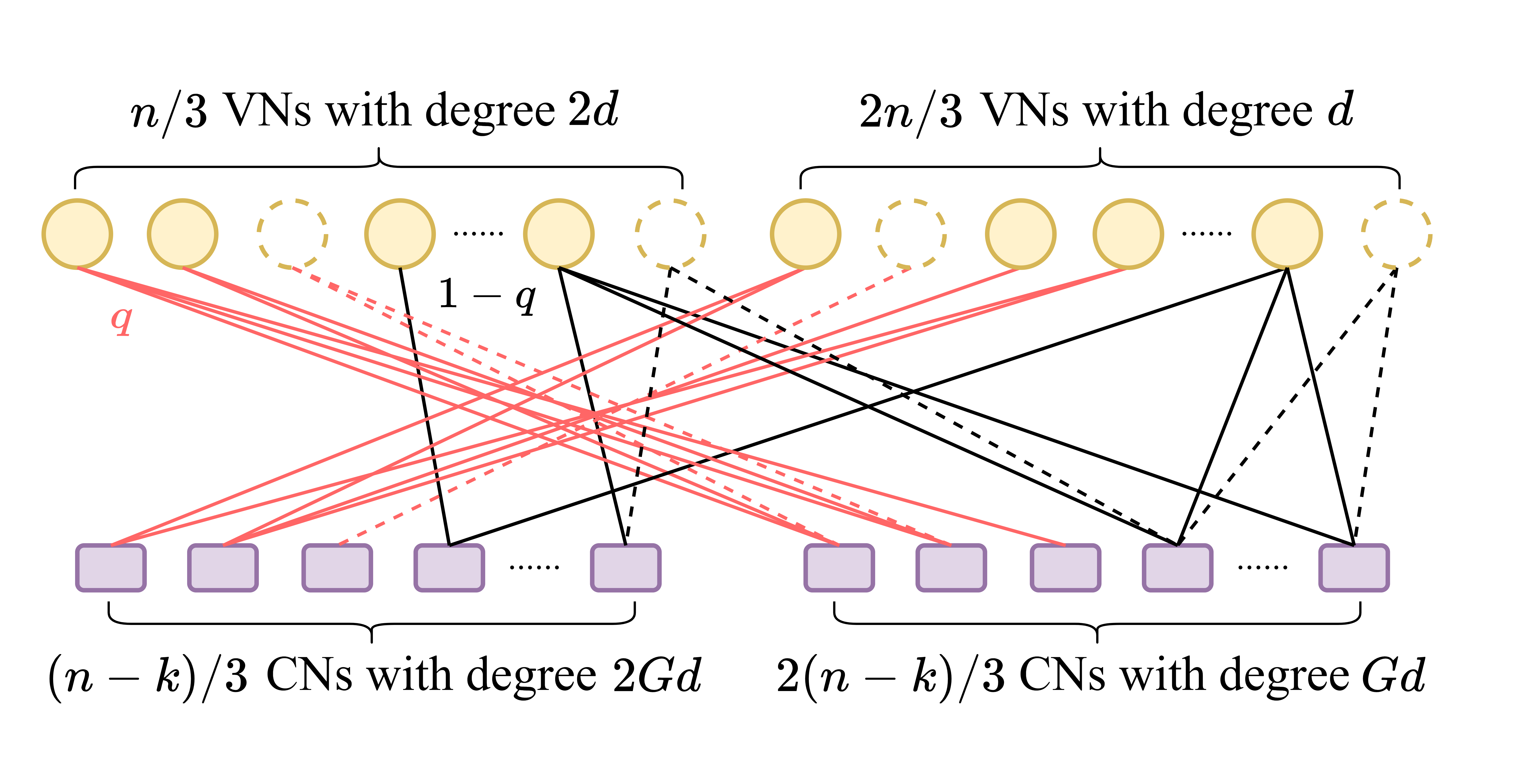
In this section, our construction for such a bipartite graph is similar to the block construction of degree-degree correlated random networks in [23]. Assume that (1) holds. We arrange the stubs of the variable nodes in descending order and partition the stubs into blocks evenly, each with stubs. In each block of stubs, we randomly select stubs as type 1 stubs, where the parameter is a design parameter for controlling the degree-degree correlation. The remaining stubs in that block are classified as type 2 stubs. Similarly, we arrange the stubs of the check nodes in descending order and partition the stubs into blocks evenly, each with stubs. In each block of stubs, we randomly select stubs as type 1 stubs and the remaining stubs as type 2 stubs. These two types of stubs will be connected differently to form degree-degree correlation.
Consider a permutation of . For , we randomly select a type 1 stub from the block of variable nodes and another type 1 stub from the block of check nodes and connect these two stubs to form an edge. Repeat the process until all the type 1 stubs are connected. For type 2 stubs, the connection is independent, i.e., we randomly select a type 2 stub of variable nodes and another type 2 stub of check nodes and connect these two stubs to form an edge. Let (resp. ) be the degree of the variable end (resp. check end) of a randomly selected edge from the bipartite graph. It is clear that the marginal distribution of the degree of the variable end (of a randomly selected edge) is
| (3) |
and the marginal distribution of the degree of the check end (of a randomly selected edge) is
| (4) |
Assume that all the nodes with the same degree are in one common block. Let (resp. ), , be the set of degrees in the block of variable nodes (resp. check nodes). Now we compute the conditional probability . Suppose that for some . If , then an edge with degree at the variable end and degree at the check end can only be formed by type 2 stubs. The number of type 2 stubs of the check nodes with degree is , and the total number of type 2 stubs is . The probability that a stub of the variable nodes is of type 2 is . Thus, for and ,
| (5) | |||||
If , then an edge with degree at the variable end and degree at the check end can also be formed by type 1 stubs. The number of type 1 stubs of the check nodes with degree is , and the total number of type 1 stubs in the block of check nodes is . The probability that a stub of the variable nodes is of type 1 is . Adding the probability formed by type 1 stubs in (5), we have for and ,
| (6) | |||||
Then, we have from (3), (4), (5), and (6) that for ,
| (9) |
Example 1
(Two types of degrees) Suppose that there are variable nodes with degree , and variable nodes with degree . Also, there are check nodes with degree , and check nodes with degree , where is a positive integer. Using the construction in Section II-A, we have , so that the condition in (1) is satisfied. Now we partition the stubs into two blocks, i.e., . The first block consists of variable nodes with degree (resp. check nodes with degree ), and the second block consists of variable nodes with degree (resp. check nodes with degree ). For the permutation with and , we have from (3) and (II-A) that
| (11) |
Note that the degree-degree correlation can be computed as follows:
| (12) |
Thus, the degree-degree correlation is negative for the permutation with and . On the other hand, it is positively correlated for the permutation with and . An illustration of the construction of the bipartite graph is shown in Figure 1, where the red (resp. black) edges are formed by type 1 (resp. 2) stubs.
II-B General construction
In this section, we propose a general construction from the degree-degree bivariate distribution . Given such a bivariate distribution, we first compute the two marginal distributions:
| (13) |
and
| (14) |
Then we use the marginal distribution in (13) and (3) to compute the degree distribution of :
| (15) |
Similarly, we have from the marginal distribution in (14) and (4) that
| (16) |
| (17) | |||||
| (18) |
Choose and so that the condition in (2) is satisfied. It then follows from (2), (3), and (4) that
| (20) |
Note that is the number of stubs of variable nodes with degree , and is the number of stubs of check nodes with degree . Among these stubs, we can randomly select stubs from the variable nodes and stubs from the check nodes, and connect them at random (as in the configuration model). As the number of edges between a variable node with degree and a check node with degree is and the total number of edges is , the probability that a randomly selected edge has degree in its variable end and degree in its check end is (cf. (II-B))
| (21) |
To provide further insight of this construction, we show an example with two types of degrees in Appendix A.
It is of interest to point out the connections between our construction and the multi-edge type LDPC codes in [24]. By classifying edges with degree in the variable end and degree in the check end into one specific type of edges, our construction is a special case of the multi-edge type LDPC codes in [24]. However, as pointed out in [24, 26], the density evolution method is generally difficult to be applied to the multi-edge type LDPC codes (as the densities of various types are convolved). By using the degree-degree bivariate distribution, we will show in Section III that one can average over the (convolved) densities of various edge types into a single node type (that only depends on its node degree). Thus, the computational complexity of the density evolution method can be greatly reduced.
III Density evolution in correlated LDPC codes
In this section, we extend the density evolution analysis for LDPC codes with degree-degree correlations. It is known that the density evolution analysis is generally difficult to be applied to the multi-edge type LDPC codes as the densities of various types are convolved. However, by using the conditional probabilities derived in the previous section, we can average over the (convolved) densities of various edge types into a single node type.
Now we derive the density evolution equations in the setting where is fixed and . Consider using a degree-degree correlated LDPC code over a binary erasure channel with the erasure probability . Let be the probability that the variable end of a randomly selected edge with degree is not decoded after the iteration, and be the probability that the check end of a randomly selected edge with degree is not decoded after the iteration. Analogous to the AND-OR argument in [8, 9], we have
| (22) |
Clearly, for all (as every variable bit is erased independently with probability through the erase channel). Similarly,
| (23) |
Combining these two equations, we have a system of nonlinear recursive equations:
| (24) |
with for all .
Let be the probability that a randomly selected variable node with degree is successfully decoded after the iteration. Note that a randomly selected variable node is not decoded after the iteration if and only if the variable node is erased and all the check ends of its edges are not decoded after the iteration. Thus,
| (25) |
Let be the probability that a randomly selected variable node is successfully decoded after the iteration. Then
As in [10], we are interested in the maximum tolerable erasure probability such that for all ,
| (27) |
Since the capacity of the BEC with the erasure probability is known to be [27], we know that . In view of (2), we have
| (28) |
In view of (III) and (23), a sufficient condition for (27) is
| (29) |
for all . In the following theorem, we show a lower bound for . The proof can be found in Appendix B.
Theorem 1
Let be the minimum degree of a variable node and be the maximum degree of a check node. If and , then for all .
IV Numerical results
IV-A Block construction
In this section, we evaluate the performance of random LDPC codes generated by the block construction in Section II-A. Consider using the randomly generated LDPC code in Example 1 for a BEC with the erasure probability . In this numerical experiment, we set , .
In Figure 2, we plot the maximum tolerable erasure probability as a function of the parameter (with the step size of 0.01) for two permutations: the negatively correlated one with (the orange curve), and the positively correlated one with (the blue curve). Recall that when , it reduces to the independent case. As shown in Figure 2, adding a negative degree-degree correlation can lead to a much larger maximum tolerable erasure probability than that of the independent case. In particular, when , we find that the maximum tolerable erasure probability is 0.3066, which is larger than for . However, adding a positive degree-degree correlation does not improve the maximum tolerable erasure probability in this numerical experiment.
To explain these numerical results, we note that LDPC codes with positive degree-degree correlations tend to form a giant component in the bipartite graph (as nodes with large degrees tend to connect to nodes with large degrees), and that makes the decoding of the LDPC code difficult. On the other hand, LDPC codes with negative degree-degree correlations are less likely to form a giant component. As such, one can exploit the negative degree-degree correlation by increasing to improve the maximum tolerable erasure probability. However, when is increased to 1, the bipartite graph gradually decouples into two separate bipartite graphs (from the block construction). Each has its own maximum tolerable erasure probability. When is close to 1, the maximum tolerable erasure probability is dominated by the bipartite graph with a smaller maximum tolerable erasure probability. Due to these two effects, the orange curve for the case with a negative degree-degree correlation is unimodal (with only one peak).

In Appendix C, we conduct extensive simulations to verify the effectiveness of the asymptotic results derived from the density evolution equations. We also show the degree’s effect on the decoding probabilities of variable nodes. One significant finding from our experiments is that the degree-degree correlation plays a critical role in unequal error protection (UEP).
IV-B General construction for performance improvement
In this section, we show that the LDPC codes from the general construction in Section II-B can lead to further performance improvement.
In [25], Shokrollahi and Storn proposed a construction of the LDPC code with the following (independent) bivariate distribution:
| (30) |
where , , , , and , . It is easy to verify that . It was shown in [25] that the maximum tolerable erasure probability .
For this example, we find the bivariate distribution , , such that it has the same marginal distributions and . The maximum tolerable erasure probability for such a bivariate distribution is 0.49568, which is larger than 0.49553 for the LDPC code in [25].
V Conclusion
In this paper, we proposed two constructions of degree-degree correlated LDPC codes and derived the density evolution equations for such LDPC codes. For the block construction, our numerical results show that adding a negative degree-degree correlation can achieve a much higher maximum tolerable erasure probability than LDPC codes with independent degree distributions. Moreover, adding a negative degree-degree correlation could lead to better designs of LDPC codes with the UEP property. The general construction (with an arbitrary bivariate degree-degree distribution) provides a much larger ensemble of LDPC codes than block construction. It can lead to performance improvement over the existing LDPC codes with independent degree-degree distributions.
References
- [1] R. Gallager, “Low-density parity-check codes,” IRE Transactions on Information Theory, vol. 8, no. 1, pp. 21–28, 1962.
- [2] J. H. Bae, A. Abotabl, H.-P. Lin, K.-B. Song, and J. Lee, “An overview of channel coding for 5g nr cellular communications,” APSIPA Transactions on Signal and Information Processing, vol. 8, 2019.
- [3] T. Thi Bao Nguyen, T. Nguyen Tan, and H. Lee, “Low-complexity high-throughput QC-LDPC decoder for 5G new radio wireless communication,” Electronics, vol. 10, no. 4, p. 516, 2021.
- [4] H.-C. Lee, J.-H. Shy, Y.-M. Chen, and Y.-L. Ueng, “LDPC coded modulation for TLC flash memory,” in 2017 IEEE Information Theory Workshop (ITW). IEEE, 2017, pp. 204–208.
- [5] Y. Fang, Y. Bu, P. Chen, F. C. Lau, and S. Al Otaibi, “Irregular-mapped protograph LDPC-coded modulation: A bandwidth-efficient solution for 6G-enabled mobile networks,” IEEE Transactions on Intelligent Transportation Systems, 2021.
- [6] N. Bonello, S. Chen, and L. Hanzo, “Low-density parity-check codes and their rateless relatives,” IEEE Communications Surveys & Tutorials, vol. 13, no. 1, pp. 3–26, 2010.
- [7] R. Tanner, “A recursive approach to low complexity codes,” IEEE Transactions on Information Theory, vol. 27, no. 5, pp. 533–547, 1981.
- [8] M. Luby, M. Mitzenmacher, and M. A. Shokrollahi, “Analysis of random processes via and-or tree evaluation,” in SODA, vol. 98, 1998, pp. 364–373.
- [9] M. Luby, M. Mitzenmacher, A. Shokrollah, and D. Spielman, “Analysis of low density codes and improved designs using irregular graphs,” in Proceedings of the thirtieth annual ACM symposium on Theory of computing, 1998, pp. 249–258.
- [10] M. A. Shokrollahi, “New sequences of linear time erasure codes approaching the channel capacity,” in International Symposium on Applied Algebra, Algebraic Algorithms, and Error-Correcting Codes. Springer, 1999, pp. 65–76.
- [11] T. J. Richardson and R. L. Urbanke, “The capacity of low-density parity-check codes under message-passing decoding,” IEEE Transactions on Information Theory, vol. 47, no. 2, pp. 599–618, 2001.
- [12] N. Rahnavard and F. Fekri, “New results on unequal error protection using LDPC codes,” IEEE Communications Letters, vol. 10, no. 1, pp. 43–45, 2006.
- [13] N. Rahnavard, H. Pishro-Nik, and F. Fekri, “Unequal error protection using partially regular LDPC codes,” IEEE Transactions on Communications, vol. 55, no. 3, pp. 387–391, 2007.
- [14] N. Rahnavard, B. N. Vellambi, and F. Fekri, “Rateless codes with unequal error protection property,” IEEE Transactions on Information Theory, vol. 53, no. 4, pp. 1521–1532, 2007.
- [15] Y.-H. Chen, Y.-T. Liu, C.-H. Wang, and C.-C. Chao, “Analysis of UEP QC-LDPC codes using density evolution,” in 2020 International Symposium on Information Theory and Its Applications (ISITA). IEEE, 2020, pp. 230–234.
- [16] Y. Zhao, Y. Zhang, F. C. Lau, Z. Zhu, and H. Yu, “Duplicated zigzag decodable fountain codes with the unequal error protection property,” Computer Communications, vol. 185, pp. 66–78, 2022.
- [17] D. J. MacKay and R. M. Neal, “Near Shannon limit performance of low density parity check codes,” Electronics letters, vol. 33, no. 6, pp. 457–458, 1997.
- [18] D. J. MacKay, “Good error-correcting codes based on very sparse matrices,” IEEE transactions on Information Theory, vol. 45, no. 2, pp. 399–431, 1999.
- [19] T. J. Richardson, M. A. Shokrollahi, and R. L. Urbanke, “Design of capacity-approaching irregular low-density parity-check codes,” IEEE Transactions on Information Theory, vol. 47, no. 2, pp. 619–637, 2001.
- [20] M. G. Luby, M. Mitzenmacher, M. A. Shokrollahi, D. A. Spielman, and V. Stemann, “Practical loss-resilient codes,” in Proceedings of the twenty-ninth annual ACM symposium on Theory of computing, 1997, pp. 150–159.
- [21] S. Giddens, M. A. Gomes, J. P. Vilela, J. L. Santos, and W. K. Harrison, “Enumeration of the degree distribution space for finite block length ldpc codes,” in ICC 2021-IEEE International Conference on Communications. IEEE, 2021, pp. 1–6.
- [22] M. Newman, Networks: an introduction. OUP Oxford, 2009.
- [23] D.-S. Lee, C.-S. Chang, M. Zhu, and H.-C. Li, “A generalized configuration model with degree correlations and its percolation analysis,” Applied Network Science, vol. 4, no. 1, pp. 1–21, 2019.
- [24] T. Richardson, R. Urbanke et al., “Multi-edge type LDPC codes,” in Workshop honoring Prof. Bob McEliece on his 60th birthday, California Institute of Technology, Pasadena, California, 2002, pp. 24–25.
- [25] A. Shokrollahi and R. Storn, “Design of efficient erasure codes with differential evolution,” in 2020 IEEE International Symposium on Information Theory (ISIT), 2000.
- [26] G. Liva and M. Chiani, “Protograph LDPC codes design based on EXIT analysis,” in IEEE GLOBECOM 2007-IEEE Global Telecommunications Conference. IEEE, 2007, pp. 3250–3254.
- [27] P. Elias, “Coding for two noisy channels,” in Proc. 3rd London Symp. Inf. Theory, Washington, DC. IEEE, 1955, pp. 61–76.
- [28] T. Richardson and R. Urbanke, Modern coding theory. Cambridge university press, 2008.
- [29] S. Kudekar, T. J. Richardson, and R. L. Urbanke, “Threshold saturation via spatial coupling: Why convolutional LDPC ensembles perform so well over the BEC,” IEEE Transactions on Information Theory, vol. 57, no. 2, pp. 803–834, 2011.
- [30] D. G. Mitchell, M. Lentmaier, and D. J. Costello, “Spatially coupled LDPC codes constructed from protographs,” IEEE Transactions on Information Theory, vol. 61, no. 9, pp. 4866–4889, 2015.
- [31] L. Bazzi, T. J. Richardson, and R. L. Urbanke, “Exact thresholds and optimal codes for the binary-symmetric channel and Gallager’s decoding algorithm A,” IEEE Transactions on Information Theory, vol. 50, no. 9, pp. 2010–2021, 2004.
Appendix A An example of two types of degrees by using the general construction
Consider the following bivariate distribution:
| (31) |
where and .
From (A), we know that
| (33) |
It is easy to see that (A) recovers (1) by letting , , and . As such, the construction in this example is more general than that in Example 1.
Similarly, from (A), it follows that
| (34) |
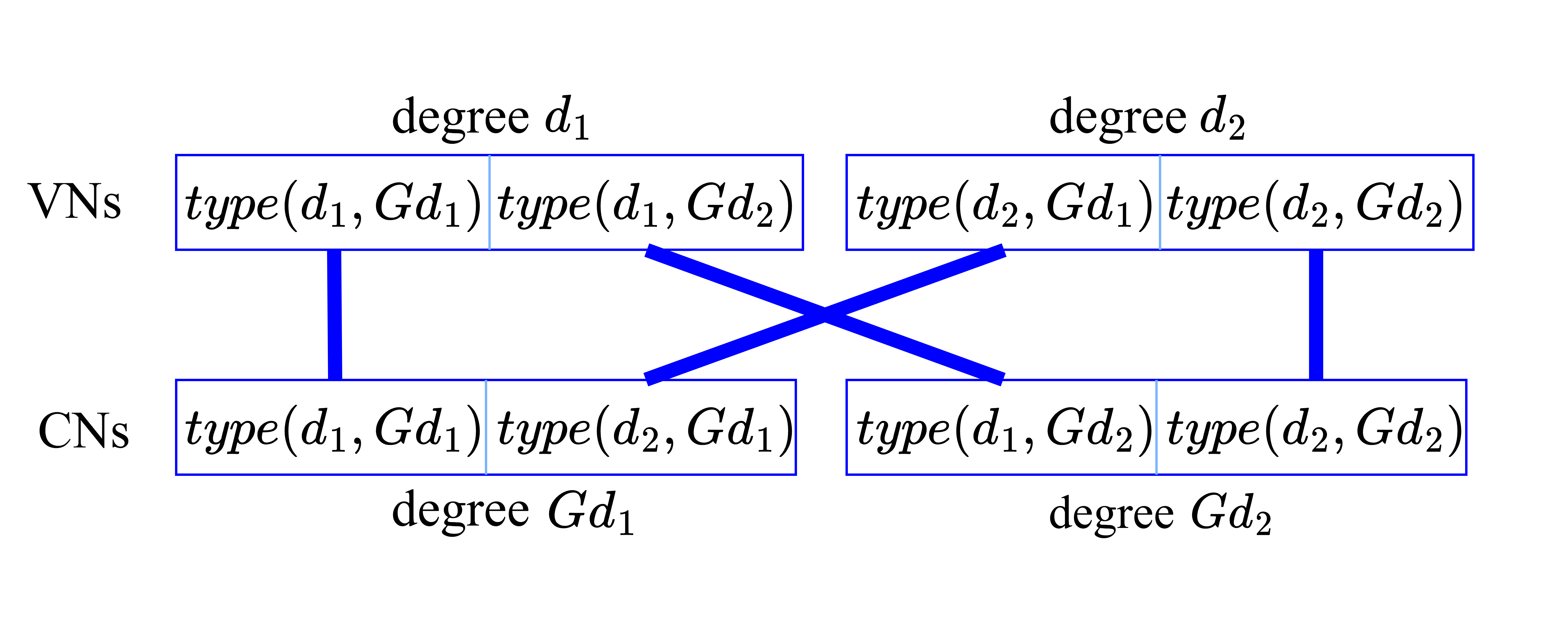
To construct a random LDPC code with the six input parameters , , , , , and in this example, one can classify the edges (with in (A)) into the four edge types (with degree in the variable end and degree in the check end): , , and . For each edge type, connect the stubs in the variable nodes and the stubs in check nodes by using the configuration model. An illustration of the construction is shown in Figure 3, where the bold lines represent edges connected among the four edge types.
Appendix B Proof of Theorem 1
Note from (23) that
| (35) |
Since , one can easily show by induction (from (23) and (22)) that for all
| (36) |
Let and . Using the inequality that for all , we have from (23) that
| (37) | |||||
It follows from (36) that
| (38) |
On the other hand, we have from (22) and (38) that
| (39) | |||||
Since we assume that , it follows from (39) that
| (40) |
Thus,
| (41) |
Since and , we have from (41) and that
| (42) |
Thus, converges to 0 when .
Appendix C Simulation results for the block construction in Section IV-A
In order to verify the effectiveness of the asymptotic results derived from the density evolution equations, we conduct extensive simulations. For our simulations, we generate degree-degree correlated LDPC codes with variable nodes and check nodes by using the construction in Example 1. Then we simulate the LDPC codes over a BEC with an erasure probability . After that, we perform iterative decoding (peeling decoder) for the LDPC codes (until there are no check nodes with degree ). In Figure 4, we plot the probability that a randomly selected variable node is successfully decoded, i.e., , as a function of the erasure probability from 0 to 0.4 with respect to various parameters , respectively. Each data point is the average of 100 experiments. The five solid curves represent the theoretical results of , and the five dotted curves represent the corresponding simulation results. As shown in Figure 4, the simulation results and the asymptotic results match very well. Also, we observe the largest maximum tolerable erasure probability occurs when (the yellow curve). This result is consistent with that of Figure 2.


Finally, we look into the effect of the degree on the decoding probabilities of variable nodes. There are two types of degrees of the variable nodes in Example 1: and . In Figure 5, we plot the probability that a randomly selected variable node with degree is successfully decoded, i.e., , as a function of the erasure probability for . The solid curve (resp. dashed curve) represents the decoding probability for a variable node with degree (resp. ). It is well-known that the decoding probability for variable nodes with a large degree is higher than that with a small degree. Such a property is known as the unequal error protection (UEP) property. One significant finding from our experiments is that the degree-degree correlation plays a critical role in UEP. Recall that the degree-degree correlation in Example 1 is . As shown in Figure 5, increasing increases the gap between the curve for and the curve for . In particular, for (the two green curves), the gap is the largest among the five choices of . Even when the erasure probability exceeds the upper bound , variable nodes with degree can still have a very high decoding probability. This is at the cost of sacrificing the decoding probability of variable nodes with degree . On the other hand, the two curves for are very close to each other. Even though they have the largest maximum tolerable erasure probability , they are not suitable for LDPC codes with the UEP property.
Appendix D Further detail for performance improvement
In this appendix, we provide the details of the performance improvement in Section IV-B.
D-1 The LDPC code by Shokrollahi and Storn [25]
In [25], Shokrollahi and Storn proposed a construction of the LDPC code with the following (independent) bivariate distribution:
| (43) |
where
| (44) |
and
| (45) |
From (17), we have
| (46) |
Thus, . From (15) and (16), we have
| (47) |
and
| (48) |
It was shown in [25] that and it is wthin less than 1% of the optimum 0.4985 (the upper bound is ).
In this numerical experiment, we conduct a search for the following set of bivariate distributions:
| (49) |
where , , and . For this example, we verify that the maximum tolerable erasure probability is with , , . Now we find the bivariate distribution , , such that it has the same marginal distributions in (D-1) and in (D-1). The maximum tolerable erasure probability for such a bivariate distribution is 0.49568, which is larger than 0.49553 for the LDPC code in [25].
D-2 The LDPC code in Example 3.63 of the book [28]
In Example 3.63 of the book [28], the LDPC code with the following (independent) bivariate distribution is considered:
| (50) |
where
| (51) |
and
| (52) |
It is easy to verify that . For such an LDPC code,
In this numerical experiment, we conduct a search for the following set of bivariate distributions:
| (53) |
where , , and . For this example, we verify that the maximum tolerable erasure probability is with , , . Now we find the bivariate distribution , , such that it has the same marginal distributions in (D-1) and in (D-1). The maximum tolerable erasure probability for such a bivariate distribution is 0.48077, which is larger than 0.47410 for the LDPC code in [28].
D-3 The LDPC code by Bazzi et al. [31]
In Example 9 of [31], Bazzi et al. considered the rate one-half LDPC code with the following (independent) bivariate distribution:
| (54) |
where
| (55) |
and
| (56) |
where is chosen to be 0.1115. From (17), we have
| (57) |
Thus, . From (15) and (16), we have
| (58) |
and
| (59) |
In this numerical experiment, we conduct a search for the following set of bivariate distributions:
| (60) |
where . For this example with , we verify that the maximum tolerable erasure probability is with . Now we find the bivariate distribution such that it has the same marginal distributions in (D-1) and in (D-1). The maximum tolerable erasure probability for such a bivariate distribution is 0.3924, which is larger than 0.3916 for the LDPC code in [31].