DEFT-FUNNEL: an open-source global optimization solver for constrained grey-box and
black-box problems
Abstract
The fast-growing need for grey-box and black-box optimization methods for constrained global optimization problems in fields such as medicine, chemistry, engineering and artificial intelligence, has contributed for the design of new efficient algorithms for finding the best possible solution. In this work, we present DEFT-FUNNEL, an open-source global optimization algorithm for general constrained grey-box and black-box problems that belongs to the class of trust-region sequential quadratic optimization algorithms. It extends the previous works by Sampaio and Toint (2015, 2016) to a global optimization solver that is able to exploit information from closed-form functions. Polynomial interpolation models are used as surrogates for the black-box functions and a clustering-based multistart strategy is applied for searching for the global minima. Numerical experiments show that DEFT-FUNNEL compares favorably with other state-of-the-art methods on two sets of benchmark problems: one set containing problems where every function is a black box and another set with problems where some of the functions and their derivatives are known to the solver. The code as well as the test sets used for experiments are available at the Github repository http://github.com/phrsampaio/deft-funnel.
Keywords Global optimization constrained nonlinear optimization black-box optimization grey-box optimization derivative-free optimization simulation-based optimization trust-region method subspace minimization sequential quadratic optimization
1 Introduction
We are interested in finding the global minimum of the optimization problem
| (5) |
where might be or not a black box, are black-box constraint functions and are white-box constraint functions. i.e. their analytical expressions as well as their derivatives are available. The vectors , , and are lower and upper bounds on the constraints values and , while and are bounds on the variables, with , , , , and . We also address the case where there are no white-box constraint functions . Finally, we assume that the bound constraints are unrelaxable, i.e. feasibility must be maintained throughout the iterations, while the other general constraints are relaxable.
When at least one of the functions in (1) has a closed form, i.e. either the objective function is a white box or there is at least one white-box constraint function in the problem, the latter is said to be a grey-box problem. If no information about the functions is given at all, which means that the objective function is a black box and that there are no white-box constraints, the problem is known as a black-box problem. Both grey-box and black-box optimization belong to the field of derivative-free optimization (DFO) [12, 4], where the derivatives of the functions are not available. DFO problems are encountered in real-life applications in various fields such as engineering, medicine, science and artificial intelligence. The black boxes are often the result of an expensive simulation or a proprietary code, in which case automatic differentiation [21, 22] is not applicable.
Many optimizations methods have been developed for finding stationary points or local minima of (1) when both the objective and the constraints functions are black boxes (e.g., [36, 29, 10, 5, 42, 43, 14, 1]). However, a local minimum is not enough sometimes and so one need to search for the global minimum [16, 15]. A reduced number of methods have been proposed to find the global minima of constrained black-box problems (see, for instance, [25, 39, 40, 37, 38, 9]) and thus there is still much research to be done on this area. Moreover, many global optimization methods for constrained black-box problems proposed in the literature or used in industry are unavailable to the public and are not open source. We refer the reader to the survey papers [41, 28] and to the textbooks [12, 4] for a comprehensive review on DFO algorithms for different types of problems.
In the case of constrained grey-box problems, especially those found in industry, it is a good idea to exploit the available information about the white boxes since such problems are usually hard to be solved, i.e. highly nonlinear, multimodal and with very expensive functions. Therefore, one would expect the solver to use any information given as input in order to attain the global minimum as fast as possible. Unfortunately, even less global optimization solvers exist for such problems today. A common solution found by optimization researchers, engineers and practioners is to consider all the functions as black boxes and to use a black-box optimization algorithm to solve the problem. Two of the few methods that exploit the available information are ARGONAUT [9] and a trust-region two-phase algorithm proposed in [6]. In ARGONAUT, the black-box functions are replaced by surrogate models and a global optimization algorithm is used to solve the problem to global optimality, having the surrogate models updated only after its resolution. After updating the models, the problem is solved again with the updated models and this process is repeated until convergence is declared. In the two-phase algorithm described in [6], radial basis functions (RBF) are used as surrogate models for the black-box functions. Moreover, as in DEFT-FUNNEL, the self-correcting geometry approach proposed by [44] is applied to the management of the interpolation set. Their algorithm is composed of a feasibility phase, where the goal is to find a feasible point, and an optimization phase, where the feasible point found in the first phase is used as a starting point to find a global minimum.
The algorithm in [6] is the one sharing more elements in common with DEFT-FUNNEL. However, these two methods are still very different in nature since DEFT-FUNNEL combines a multistart strategy with a sequential quadratic optimization (SQO) algorithm in order to find global minima while the other applies a global optimization solver in its both phases for this purpose. Besides, DEFT-FUNNEL employs local polynomial interpolation models rather than RBF models as the former have good performance in the context of local optimization, which suits well for the SQO algorithm used in its local search. Despite the good performance of the algorithms proposed in [9] and [6], neither is freely available or open source.
Contributions. This paper proposes a new global optimization solver for general constrained grey-box and black-box problems written in Matlab [32] that exploits any available information given as input and that employs surrogate models built from polynomial interpolation in a trust-region-based SQO algorithm. Differently from the ARGONAUT approach, the surrogate models are updated during the optimization process as soon as new information from the evaluation of the functions at the iterates become available. Furthermore, the proposed solver, named DEFT-FUNNEL, is open source and freely available at the Github repository http://github.com/phrsampaio/deft-funnel. It is based on the previous works in [42, 43] and it extends the original DFO algorithm to grey-box problems and to the search for global minima. As its previous versions, it does not require feasible starting points. To our knowledge, DEFT-FUNNEL is the first open-source global optimization solver for general constrained grey-box and black-box problems that exploits the derivative information available from the white-box functions. It is also the first one of the class of trust-funnel algorithms [19] to be used in the search for global minima in both derivative-based and derivative-free optimization.
This paper serves also as the first release of the DEFT-FUNNEL code to the open-source community and to the public in general. For this reason and also due to the new extensions mentioned above, we give a complete description of the algorithm so that the reader can understand the method more easily while examining the code on Github. We also notice that some modifications and additions have been made to the local-search SQO algorithm with respect to the one presented in [43]. In particular, some changes were done in the condition for the normal step calculation, in the criticality step and in the maintenance of the interpolation set, all of them being described in due course. Furthermore, we have also added a second-order correction step.
The extension to global optimization is based on the multi-level single linkage (MLSL) method [26, 27], a well-known stochastic multistart strategy that combines random sampling, a clustering-based approach for the selection of the starting points and local searches in order to identify all local minima. In DEFT-FUNNEL, it is used for selecting the starting points of the local searches done with the trust-funnel SQO algorithm.
Organization. The outline of this paper is as follows. Section 2 introduces the MLSL method while in Section 3 the DEFT-FUNNEL solver is presented in detail. In Section 4, numerical results on a set of benchmark problems for global optimization are shown and the performance of DEFT-FUNNEL is compared with those of other state-of-the-art algorithms in a black-box setting. Moreover, numerical results on a set of grey-box problems are also analyzed. Finally, some conclusions about the proposed solver are drawn in Section 5.
Notation. Unless otherwise specified, the norm is the standard Euclidean norm. Given any vector , we denote its -th component by . We define where the operation is done componentwise. We let denote the closed Euclidian ball centered at z, with radius . Given any set , denotes the cardinality of . By , we mean the space of all polynomials of degree at most in . Finally, given any subspace , we denote its dimension by .
2 Multi-level single linkage
The MLSL method [26, 27] is a stochastic multistart strategy originally designed for bound-constrained global optimization problems as below
| (8) |
where is a convex, compact set containing the global minimum as an interior point that is defined by lower and upper bounds. It was later extended to problems with general constraints in [45]. As most of the stochastic multistart methods, it consists of a global phase, where random points are sampled from a probabilistic distribution, and a local phase, where selected points from the global phase are used as starting points for local searches done by some local optimization algorithm. MLSL aims at avoiding unnecessary and costly local searches that culminate in the same local minima. To achieve this goal, sample points are drawn from an uniform distribution in the global phase and then a local search procedure is applied to each of them except if there is another sample point or a previously detected local minimum within a critical distance with smaller objective function value. The method is fully described in Algorithm 2.
Algorithm 2.1: MLSL
- 1:
-
- 2:
-
for to do
- 3:
-
Generate random points uniformly distributed.
- 4:
-
Rank the sample points by increasing value of .
- 5:
-
for to do
- 6:
-
if and then
- 7:
-
- 8:
-
end if
- 9:
-
end for
- 10:
-
end for
- 11:
-
return the best local minimum found in
The critical distance is defined as
| (9) |
where is the gamma function and is the Lebesgue measure of the set . The method is centred on the idea of exploring the region of attraction of all local minima, which is formally defined below.
Definition 2.1.
Given a local search procedure , we define a region of attraction in to be the set of all points in starting from which will arrive at .
The ideal multistart method is the one that runs a local search only once at the region of attraction of every local minimum. However, two types of errors might occur in practice [30]:
-
•
Error 1. The same local minimum has been found after applying local search to two or more points belonging to the same region of attraction of .
-
•
Error 2. The region of attraction of a local minimum contains at least one sampled point, but local search has never been applied to points in this region.
In [26, 27], the authors demonstrate the following theoretical properties of MLSL that are directly linked to the errors above:
- •
- •
Property 1 states that the number of possible occurrences of Error 1 is finite while Property 2 says that Error 2 never happens. Due to its strong theoretical results and good practical performance, MLSL became one of the most reliable and popular multistart methods of late.
Finally, we note that MLSL has already been applied into the global constrained black-box optimization setting in [2]. The proposed method, MLSL-MADS, integrates MLSL with a mesh adaptive direct search (MADS) method [3] to find multiple local minima of an inverse transport problem involving black-box functions.
3 The DEFT-FUNNEL solver
We first define the function as , i.e. it includes all the constraint functions of the original problem (5). Then, by defining and , the problem (5) is rewritten as
| (14) |
where are slack variables and and are the lower and upper bounds of the modified problem with and . We highlight that the rewriting of the original problem (5) as (14) is done within the solver and that the user does not need to interfere.
DEFT-FUNNEL is composed of a global search and a local search that are combined to solve the problem (14). In the next two sections, we elaborate on each of these search steps.
3.1 Global search
As mentioned previously, the global search in DEFT-FUNNEL relies on the MLSL multistart strategy. A merit function is used to decide which starting points are selected for the local search. We introduce the global search in detail in what follows.
Algorithm 3.1: GlobalSearch
- 1:
-
- 2:
-
for to do
- 3:
-
Generate random points uniformly distributed.
- 4:
-
Rank the sample points by increasing value of .
- 5:
-
for to do
- 6:
-
if and then
- 7:
-
- 8:
-
end if
- 9:
-
end for
- 10:
-
end for
- 11:
-
return the best feasible local minimum found in
The Algorithm 3.1 is implemented in the function deft_funnel_multistart, which is called by typing the following line in the Matlab command window:
The inputs and outputs of deft_funnel_multistart are detailed in Table 1. The options for the input ‘whichmodel’ are described in Section 3.2.
| Name | Description | |
|---|---|---|
| Mandatory | f | function handle of the objective function |
| Inputs | c | function handle of the black-box constraints if any or an empty array |
| h | function handle of the white-box constraints if any or an empty array | |
| dev_f | function handle of the derivatives of f if it is a white box or an empty array | |
| dev_h | function handle of the derivatives of h if any or an empty array | |
| n | number of decision variables | |
| nb_cons_c | number of black-box constraints (bound constraints not included) | |
| nb_cons_h | number of white-box constraints (bound constraints not included) | |
| Optional | lsbounds | vector of lower bounds for the constraints |
| Inputs | usbounds | vector of upper bounds for the constraints |
| lxbounds | vector of lower bounds for the x variables | |
| uxbounds | vector of upper bounds for the x variables | |
| maxeval | maximum number of evaluations (default: 5000*n) | |
| maxeval_ls | maximum number of evaluations per local search (default: maxeval*0.7) | |
| whichmodel | approach to build the surrogate models | |
| f_global_optimum | known objective function value of the global optimum | |
| Outputs | best_sol | best feasible solution found |
| best_fval | objective function value of “best_sol” | |
| best_indicators | indicators of “best_sol” | |
| total_eval | number of evaluations used | |
| nb_local_searches | number of local searches done | |
| fL | objective function values of all local minima found |
The merit function employed in DEFT-FUNNEL is the well-known penalty functon which is defined as follows:
| (15) |
where is the total number of constraints and is the penalty parameter. One of the advantages of this penalty function over others is that it is exact, that is, for sufficiently large values of , the local minimum of subject only to the bound constraints on the variables is also the local minimum of the original constrained problem (5). We note that, although is nondifferentiable, it is only used in the global search for selecting the starting points for the local searches.
The LocalSearch algorithm at line 7 is started by calling the function deft_funnel whose inputs and outputs are given in the next section.
3.2 Local search
The algorithm used in the local search is based on the one described in the paper [43]. It is a trust-region SQO method that makes use of a funnel bound on the infeasibility of the iterates in order to ensure convergence. At each iteration , we have an iterate such that , where defines the interpolation set at iteration . Every iterate satisfies the following bound constraints:
| (16) | |||
| (17) |
Depending on the optimality and feasibility of , a new step is computed. Each full step of the trust-funnel algorithm is decomposed as
| (24) |
where the normal step component aims to improve feasibility and the tangent step component reduces the objective function model without worsening the constraint violation up to first order. This is done by requiring the tangent step to lie in the null space of the Jacobian of the constraints and by requiring the predicted improvement in the objective function obtained in the tangent step to not be negligible compared to the predicted change in resulting from the normal step. The full composite step is illustrated in Figure 1. As it is explained in the next subsections, the computation of the composite step in our algorithm does not involve the function itself but rather its surrogate model.
After having computed a trial point , the algorithm proceeds by checking whether the iteration was successful in a sense yet to be defined. The iterate is then updated correspondingly, while the sample set and the trust regions are updated according to a self-correcting geometry scheme to be described later on. If has been modified, the surrogate models are updated to satisfy the interpolation conditions for the new set , implying that new function evaluations are carried out for the additional point obtained at iteration .

The local search is started inside the multistart strategy loop in Algorithm 3.1, but it can also be called directly by the user in order to use DEFT-FUNNEL without multistart. This is done by typing the following line at the Matlab command window:
The inputs and outputs of the function deft_funnel are detailed below in Table 2. Many other additional parameters can be set directly in the function deft_funnel_set_parameters. Those are related to the trust-region mechanism, to the interpolation set maintenance and to criticality step thresholds.
| Name | Description | |
|---|---|---|
| Mandatory | f | function handle of the objective function |
| Inputs | c | function handle of the black-box constraints if any or an empty array |
| h | function handle of the white-box constraints if any or an empty array | |
| dev_f | function handle of the derivatives of f if it is a white box or an empty array | |
| dev_h | function handle of the derivatives of h if any or an empty array | |
| x0 | starting point (no need to be feasible) | |
| nb_cons_c | number of black-box constraints (bound constraints not included) | |
| nb_cons_h | number of white-box constraints (bound constraints not included) | |
| Optional | lsbounds | vector of lower bounds for the constraints |
| Inputs | usbounds | vector of upper bounds for the constraints |
| lxbounds | vector of lower bounds for the x variables | |
| uxbounds | vector of upper bounds for the x variables | |
| maxeval | maximum number of evaluations (default: 500*n) | |
| type_f | string ’BB’ if f is a black box (default) or ’WB’ otherwise | |
| whichmodel | approach to build the surrogate models | |
| Outputs | x | the best approximation found to a local minimum |
| fx | the value of the objective function at x | |
| mu | local estimates for the Lagrange multipliers | |
| indicators | feasibility and optimality indicators | |
| evaluations | number of calls to the objective function and constraints | |
| iterate | info related to the best point found as well as the coordinates of all past iterates | |
| exit_algo | output signal (0: terminated with success; -1: terminated with errors) |
Once the initial interpolation set has been built using one of the methods described in the next subsection, the algorithm calls the function deft_funnel_main. In fact, deft_funnel serves only as a wrapper for the main function of the local search, deft_funnel_main, doing all the data preprocessing and paramaters setting needed in the initialization process. All the main steps such as the subspace minimization step, the criticality step and the computation of the new directions are part of the scope of deft_funnel_main.
3.2.1 Building the surrogate models
The local-search algorithm starts by building an initial interpolation set either from a simplex or by drawing samples from an uniform distribution. The construction of the interpolation set is done in the function deft_funnel_build_initial_sample_set, which is called only once during a local search within deft_funnel. The choice between random sampling and simplex is done in deft_funnel when calling the function deft_funnel_set_parameters, which defines the majority of parameters of the local search. If random sampling is chosen, it checks if the resulting interpolation set is well poised and, if not, it is updated using the Algorithm 6.3 described in Chapter 6 in [12], which is implemented in deft_funnel_repair_Y.
For the sake of simplicity, we assume henceforth that the objective function is also a black box. Given a poised set of sample points with an initial point , the next step of our algorithm is to replace the objective function and the black-box constraint functions by surrogate models and built from the solution of the interpolation system
| (25) |
where
where is the basis of monomials and is replaced by the objective function or some black-box constraint function .
We consider underdetermined quadratic interpolation models that are fully linear and that are enhanced with curvature information along the optimization process. Since the linear system (25) is potentially underdetermined, the resulting interpolating polynomials will be no longer unique and so we provide to the user four approaches to construct the models and that can be chosen by passing a number from 1 to 4 to the input ‘whichmodel’: 1 - subbasis selection approach; 2 - minimum -norm models (by defatul); 3 - minimum Frobenius norm models; and 4 - regression mnodels (recommended for noisy functions). Further details about each one can be found in [12].
If , a linear model rather than an underdetermined quadratic model is built for each function. The reason is that, despite both having error bounds that are linear in for the first derivatives, the error bound for the latter includes also the norm of the model Hessian, as stated in Lemma 2.2 in [46], which makes it worse than the former.
Whenever , the algorithm builds underdetermined quadratic models based on the choice of the user between the approaches described above. If regression models are considered instead, we set , which means that the sample set is allowed to have twice the number of sample points required for fully quadratic interpolation models. Notice that having a number of sample points much larger than the required for quadratic interpolation can also worsen the quality of the interpolation models as the sample set could contain points that are too far from the iterate, which is not ideal for models built for local approximation.
It is also possible to choose the initial degree of the models
between fully linear, quadratic with a diagonal Hessian or fully quadratic. This is done within deft_funnel by setting the input argument cur_degree in the call to deft_funnel_set_parameters to one of the following options: model_size.plin, model_size.pdiag or model_size.pquad.
The interpolation system (25) is solved using a QR factorization of the matrix within the function deft_funnel_computeP, which is called by deft_funnel_build_models.
In order to evaluate the error of the interpolation models and their derivatives with respect to the original functions and , we make use of the measure of well poisedness of given below.
Definition 3.1.
Let be a poised interpolation set and be a space of polynomials of degree less than or equal to on . Let and be the basis of Lagrange polynomials associated with . Then, the set is said to be -poised in for (in the interpolation sense) if and only if
As it is shown in [12], the error bounds for at most fully quadratic models depend linearly on the constant ; the smaller it is, the better the interpolation models approximate the original functions. We also note that the error bounds for undetermined quadratic interpolation models are linear in the diameter of the smallest ball containing for the first derivatives and quadratic for the function values.
Finally, since the constraint functions are replaced by surrogate models in the algorithm, we define the models and , which are those used for computing new directions.
3.2.2 Subspace minimization
In this subsection, we explain how the subspace minimization is employed in our algorithm. We define the subspace at iteration as
where and define the index sets of (nearly) active variables at their bounds, for some small constant . If or , a new well-poised interpolation set is built and a recursive call is made in order to solve the problem in the new subspace .
If the algorithm converges in a subspace with an optimal solution , it checks if the latter is also optimal for the full-space problem, in which case the algorithm stops. If not, the algorithm continues by attempting to compute a new direction in the full space. This procedure is illustrated in Figure 2.

The dimensionality reduction of the problem mitigates the chances of degeneration of the interpolation set when the sample points become too close to each other and thus affinely dependent. Figure 3 gives an example of this scenario as the optimal solution is approached.

In order to check the criticality in the full-space problem, a full-space interpolation set of degree is built in an -neighborhood around the point , which is obtained by assembling the subspace solution and the fixed components . The models and are then updated and the criticality step is entered.
The complete subspace minimization step is described in Algorithm 3.2.2 and it is implemented in the function deft_funnel_subspace_min, which is called inside deft_funnel_main.
Algorithm 3.2: SubspaceMinimization(, , , , , , )
- 1:
-
Check for (nearly) active bounds at and define . If there is no (nearly) active bound or if has already been explored, go to Step 5. If all bounds are active, go to Step 4.
- 2:
-
Build a new interpolation set in .
- 3:
-
Call recursively LocalSearch(, , , , , , ) and let be the solution of the subspace problem after adding the fixed components.
- 4:
-
If , return . Otherwise, reset , construct new set around , build and and recompute (optimality measure).
- 5:
-
If has already been explored, set , reduce the trust regions radii and , set and build a new poised set in .
3.2.3 The normal step
The normal step aims at reducing the constraint violation at given point defined by
| (26) |
To ensure that the step is normal to the linearized constraint , where is the Jacobian of with respect to and is the Jacobian of with respect to , we require that
| (27) |
for some .
The computation of is done by solving the constrained linear least-squares subproblem
| (33) |
where
| (34) |
for some trust-region radius . Finally, a funnel bound is imposed on the constraint violation for the acceptance of new iterates to ensure the convergence towards feasibility.
We notice that, although a linear approximation of the constraints is used for calculating the normal step, the second-order information of the quadratic interpolation model is still used in the SQO model employed in the tangent step problem as it is shown next.
The subproblem (33) is solved within the function deft_funnel_normal_step, which makes use of an original active-set algorithm where the unconstrained problem is solved at each iteration in the subspace defined by the currently active bounds, themselves being determined by a projected Cauchy step. Each subspace solution is then computed using a SVD decomposition of the reduced matrix. This algorithm is implemented in the function deft_funnel_blls and is intended for small-scale bound-constrained linear least-squares problems.
3.2.4 The tangent step
The tangent step is a direction that improves optimality and it is computed by using a SQO model for the problem (14) after the normal step calculation. The quadratic model for the function objective function is defined as
| (35) |
where , , and is the approximate Hessian of the Lagrangian function
with respect to , given by
| (36) |
where and are the Lagrange multipliers associated to the lower and upper bounds, respectively, on the slack variables , and and , the Lagrange multipliers associated to the lower and upper bounds on the variables. In (36), , and the vector may be viewed as a local approximation of the Lagrange multipliers with respect to the equality constraints .
By applying (24) into (35), we obtain
| (37) |
where
| (38) |
Since (37) is a local approximation for the function , a trust region with radius is used for the complete step :
| (39) |
Moreover, given that the normal step was also calculated using local models, it makes sense to remain in the intersection of both trust regions, which implies that
| (40) |
where .
In order to make sure that there is still enough space left for the tangent step within , we first check if the following constraint on the normal step is satisfied:
| (41) |
for some . If (41) holds, the tangent step is calculated by solving the following subproblem
| (48) |
where we require that the new iterate belongs to subspace and that it satisfies the bound constraints (16) and (17). In the Matlab code, the tangent step is calculated by the function deft_funnel_tangent_step, which in turn calls either the Matlab solver linprog or our implementation of the nonmonotone spectral projected gradient method [8] in deft_funnel_spg to solve the subproblem (48). The choice between both solvers is based on whether , for a small , in which case we assume that the problem is linear and therefore linprog is used.
We define our -criticality measure as
| (49) |
where is the projected Cauchy direction obtained by solving the linear optimization problem
| (56) |
By definition, measures how much decrease could be obtained locally
along the projection of the negative of the approximate gradient onto the nullspace of intersected with the region delimited by the bounds. This measure is computed in deft_funnel_compute_optimality, which uses lingprog to solve the subproblem (56).
A new local estimate of the Lagrange multipliers are computed by solving the following problem:
| (59) |
where
| (73) | |||||
the matrix is the identity matrix, the matrices and are obtained from by removing the columns whose indices are not associated to any active (lower and upper, respectively) bound at , the matrices and are obtained from the identity matrix by removing the columns whose indices are not associated to any active (lower and upper, respectively) bound at , and the Lagrange multipliers are those in associated to active bounds at and . All the other Lagrange multipliers are set to zero.
The subproblem (59) is also solved using the active-set algorithm implemented in the function deft_funnel_blls.
3.2.5 Which steps to compute and retain
The algorithm computes normal and tangent steps depending on the measures of feasibility and optimality at each iteration. Differently from [42, 43], where the computation of the normal steps depends on the measure of optimality, here the normal step is computed whenever the following condition holds
| (74) |
for some small , i.e. preference is always given to feasibility. This choice is based on the fact that, in many real-life problems with expensive functions and a small budget, one seeks to find a feasible solution as fast as possible and that a solution having a smaller objective function value than the current strategy is already enough. If (74) fails, we set .
We define a -criticality measure that indicates how much decrease could be obtained locally along the projection of the negative gradient of the Gauss-Newton model of at onto the region delimited by the bounds as
where the projected Cauchy direction is given by the solution of
| (80) |
We say that is an infeasible stationary point if and , in which case the algorithm terminates.
The procedure for the calculation of the normal step is given in the algorithm below. In the code, it is implemented in the function deft_funnel_normal_step, which calls the algorithm in deft_funnel_blls in order to solve the normal step subproblem (33).
Algorithm 3.3: NormalStep(, , , , )
- 1:
-
If and , STOP (infeasible stationary point).
- 2:
If the solution of (56) is , then by (49) we have , in which case we set . If the current iterate is farther from feasibility than from optimality, i.e., for a given a monotonic bounding function , the condition
| (81) |
fails, then we skip the tangent step computation by setting .
After the computation of the tangent step, the usefulness of the latter is evaluated by checking if the following conditions
| (82) |
and
| (83) |
where
| (84) |
and
| (85) |
are satisfied for some and for . The inequality (83) indicates that the predicted improvement in the objective function obtained in the tangent step is substantial compared to the predicted change in resulting from the normal step. If (82) holds but (83) fails, the tangent step is not useful in the sense just discussed, and we choose to ignore it by resetting .
The tangent step procedure is stated in Algorithm 3.2.5 and it is implemented in the function deft_funnel_tangent_step.
Algorithm 3.4: TangentStep(, , )
- 1:
- 2:
- 3:
-
Define .
3.2.6 Iteration types
Depending on the contributions of the current iteration in terms of optimality and feasibility, we classify it into three types: -iteration, -iteration and -iteration. This is done by checking if some conditions hold for the trial point defined as
| (86) |
3.2.6.1 -iteration
If , which means that the Lagrange multiplier estimates are the only new values that have been computed, iteration is said to be a -iteration with reference to the Lagrange multipliers associated to the constraints . Notice, however, that not only new values have been computed, but all the other Lagrange multipliers as well.
In this case, we set , , , and we use the new multipliers to build a new SQO model in (35).
Since null steps might be due to the poor quality of the interpolation models, we check the -poisedness in -iterations and attempt to improve it whenever the following condition holds
| (87) |
where
and . The inequality (87) gives an estimate of the error bound for the interpolation models. If (87) holds, we try to reduce the value at the left side by modifying the sample set . Firstly, we choose a constant and replace all points such that
by new points that (approximately) maximizes in . Then we use the Algorithm 6.3 described in Chapter 6 in [12] with the smaller region to improve -poisedness of the new sample set. This procedure is implemented in the Matlab code by the function deft_funnel_repair_sample_set.
3.2.6.2 -iteration
If iteration has mainly contributed to optimality, we say that iteration is an -iteration. Formally, this happens when , (83) holds, and
| (88) |
Convergence of the algorithm towards feasibility is ensured by condition (88), which limits the constraint violation with the funnel bound.
In this case, we set ) if
| (89) |
and ) otherwise. Note that (because of (84) and (83)) unless is first-order critical, and hence that condition (89) is well-defined. As for the value of the funnel bound, we set .
Since our method can suffer from the Maratos effect [31], we also apply a second-order correction (see Chapter 15, Section 15.6, in [35] for more details) to the normal step whenever the complete direction is unsuccessful at improving optimality, i.e., whenever the condition (89) fails. As the latter might be due to the local approximation of the constraint functions, this effect may be overcome with a second-order step that is calculated in deft_funnel_sec_order_correction by solving the following subproblem
| (95) |
where
| (96) |
3.2.6.3 -iteration
If iteration is neither a -iteration nor a -iteration, then it is said to be a -iteration. This means that the major contribution of iteration is to improve feasibility, which happens when either or when (83) fails.
We accept the trial point if the improvement in feasibility is comparable to its predicted value
and the latter is itself comparable to its predicted decrease along the normal step, that is
| (97) |
for some and where
| (98) |
If (97) fails, the trial point is rejected.
Finally, the funnel bound is updated as follows
| (101) |
for some and .
3.2.7 Criticality step
Two different criticality steps are employed: one for the subspaces with and one for the full space (). In the latter, convergence is declared whenever at least one of the following conditions is satisfied: (1) the trust-region radius is too small, (2) the computed direction is too small or (3) both feasibility and optimality have been achieved and the error between the real functions and the models is expected to be sufficiently small. As it was mentioned before, this error is directly linked to the -poisedness measure given in Definition 3.1. In the subspace, we are less demanding and only ask that either be very small or both feasibility and optimality have been achieved without checking the models error though.
The complete criticality step in DEFT-FUNNEL is described in the next algorithm.
Algorithm 3.5: CriticalityStep(, , , )
- Step 1:
-
If ,
- Step 1.1:
-
If , return .
- Step 1.2:
-
If and , return .
- Step 2:
-
If ,
- Step 2.1:
-
If or , return .
- Step 2.2:
-
Define , and .
- Step 2.3:
-
If and , set and modify as needed to ensure it is -poised in . If was modified, compute new models and , calculate and and increment by one. If and , return ; otherwise, start Step 2.3 again;
- Step 2.4:
-
Set , , , and define if a new model has been computed.
3.3 Maintenance of the interpolation set and trust-region updating strategy
The management of the geometry of the interpolation set is based on the self-correcting geometry scheme proposed in [44], where unsuccessful trial points are used to improve the geometry of the interpolation set. It depends on the criterion used to define successful iterations, which is passed to the algorithm through the parameter criterion. This parameter depends on the iteration type (, or , as explained previously). In general, unsuccessful trial points replace other sample points in the interpolation set which maximize a combined criteria of distance and poisedness involving the trial point. Finally, we also notice that we do not make use of “dummy” interpolation points resulting from projections onto the subspaces as in [43] anymore. The whole procedure is described in Algorithm 3.3. The definition of the maximum cardinality of the interpolation set, , is given in Section 3.2.1.
Algorithm 3.6: UpdateInterpolationSet(, , , , , criterion)
- 1: Augment the interpolation set.
-
If , then define .
- 2: Successful iteration.
-
If and criterion holds, then define for
(102) - 3: Replace a far interpolation point.
-
If , criterion fails, either or , and the set
(103) is non-empty, then define , where
(104) - 4: Replace a close interpolation point.
-
If , criterion fails, either or , the set is empty, and the set
(105) is non-empty, then define , where
(106) - 5: No replacements.
-
If , criterion fails and either [ and ] or , then define .
The trust-region update strategy associated to - and -iterations are now described. Following the idea proposed in [20], the trust-region radii are allowed to decrease even when the interpolation set has been changed after the replacement of a far point or a close point at unsuccessful iterations. However, the number of times it can be shrunk in this case is limited to and as a means to prevent the trust regions from becoming too small. If the interpolation set has not been updated, the algorithm understands that the lack of success is not due to the surrogate models but rather to the trust region size and thus it reduces the latter.
Algorithm 3.7: -iteration(, , , , , )
- 1: Successful iteration.
-
If , set and . The radius of is updated by
(109) The radius of is updated by
(112) - 2: Unsuccessful iteration.
-
If , set and . The radius of is updated by
(116) If and , update .
The operations related to -iterations follow below.
Algorithm 3.8: -iteration(, , , , , )
- 1: Successful iteration.
-
If (97) holds, set , and . The radius of is updated by
(119) - 2: Unsuccessful iteration.
-
If (97) fails, set and . The radius of is updated by
(124) If and , update .
3.3.1 The local-search algorithm
We now provide the full description of the local search which assembles all the previous subroutines.
Algorithm 3.9: LocalSearch(, , , , , , )
- 0: Initialization.
-
Choose an initial vector of Lagrange multipliers and parameters , , , , , , , , , , . Define . Initialize , with and , as well as the maximum number of interpolation points . Compute the associated models and around and Lagrange polynomials . Set . Define , where and . Compute by solving (56) with normal step and define as in (49). Define and and set . Set and .
- 1:
-
SubspaceMinimization(, , , , , , ).
- 2:
-
CriticalityStep(, , , ).
- 3:
-
NormalStep(, , , , ).
- 4:
-
TangentStep(, , ).
- 5: Conclude a -iteration.
-
If , then
- 5.1:
-
set , and ;
- 5.2:
-
set , and .
- 6: Conclude an -iteration.
- 7: Conclude a -iteration.
- 8: Update the models and the Lagrange polynomials.
-
If , compute the interpolation models and around using and the associated Lagrange polynomials . Increment by one and go to Step 1.
3.4 Parameters tuning and user goals
Like any other algorithm, DEFT-FUNNEL performance can be affected by how its parameters are tuned. In this section, we discuss about which parameters might have a major impact in its performance and how they should be tuned depending on the user goals. We consider four main aspects concerning the resolution of black-box problems: the budget, the priority level given to feasibility, the type of the objective function and the priority level given to global optimality. We can then describe the possible scenarios in decreasing order of difficulty as below:
-
•
Budget: very low, limited or unlimited.
-
•
Priority to feasibility: high or low.
-
•
Objective function: highly multimodal, multimodal or unimodal.
-
•
Priority given to global optimality: high or low.
Clearly, if the objective function is highly multimodal and the budget is limited, one should give priority to a multistart strategy with a high number of samples per iteration in case where global optimality is important. This can be done via two ways: the first one is by reducing the budget for each local search through the optional input maxeval_ls, which equals maxeval*0.7 by default; for instance, one could try setting maxeval_ls = maxeval*0.4, so that each local search uses up to 40% of the total budget only. The other possibility is to increase the number of random points generated at Step 3 in the global search (see Algorithm 3.1). In case where attaining the global minimum is not a condition, a better approach would be to give more budget to each local search so that the chances to reach a local minimum are higher. If the objective function is not highly multimodal, one should search for a good compromise between spending the budget on each local search and on the sampling of the multistart strategy.
We also notice that when the budget is too small and it is very hard to find a feasible solution, it may be a good idea to compute a tangent step only when feasibility has been achieved. This is due to the fact that tangent steps may still deteriorate the gains in feasibility obtained through normal steps. When this happens, more normal steps must be computed which requires more function evaluations. Therefore, instead of spending the budget with both tangent and normal steps without guarantee of feasibility in the end, it is a better strategy to compute only normal steps in the beginning so that the chances of obtaining a feasible solution are higher in the end. For this purpose, the user should set the constant value in (41). By doing so, the tangent step will be computed only if the normal step equals zero, which by (74) it happens when the iterate is feasible. In the code, this can be done by setting kappa_r to zero in the function deft_funnel_set_parameters.
4 Numerical experiments
We divide the numerical experiments into two sections: the first one is focused on the evaluation of the performance of DEFT-FUNNEL on black-box optimization problems, while the second one aims at analyzing the benefits of the exploitation of white-box functions on grey-box problems. In all experiments with DEFT-FUNNEL, minimum -norm models were employed. The criticality step threshold was set to and the trust-region constants were defined as , , , , , and , where is the number of variables.
We compare DEFT-FUNNEL with two popular algorithms for constrained black-box optimization: the Genetic Algorithm (GA) and the Pattern Search (PS) algorithm from the Matlab Global Optimization Toolbox [32]. In particular, GA has been set with the Adaptive Feasible (’mutationadaptfeasible’) default mutation function and the Penalty (’penalty’) nonlinear constraint algorithm. As for PS, since it is a local optimization algorithm, it has been coupled with the Latin Hypercube Sampling (LHS) [33] method in order to achieve global optimality, a common strategy found among practitioners. Our experiments cover therefore three of the most popular approaches for solving black-box problems: surrogate-based methods, genetic algorithms and pattern-search methods. Other DFO algorithms have already been compared against DEFT-FUNNEL in previous papers (see [42, 43]) on a much larger set of test problems mainly designed for local optimization.
4.1 Black-box optimization problems
The three methods are compared on a set of 14 well-known benchmark problems for constrained global optimization, including four industrial design problems — Welded Beam Design (WB4) [13], Gas Transmission Compressor Design (GTCD4) [7], Pressure Vessel Design (PVD4) [11] and Speed Reducer Design (SR7) [17] — and the Harley pooling problem (problem 5.2.2 from [16]), which is originally a maximization problem and that has been converted into a minimization one. Besides the test problems originated from industrial applications, we have collected problems with different characteristics (multimodal, nonlinear, separable and non-separable, with connected and disconnected feasible regions) to have a broader view of the performance of the algorithms in various kinds of scenarios. For instance, the Hesse problem [23] is the result of the combination of 3 separable problems with 18 local minima and 1 global minimum, while the Gómez #3 problem, listed as the third problem in [18], consists of many disconnected feasible regions, thus having many local minima. The test problems G3-G11 are taken from the widely known benchmark list in [34]. In Table 3, we give the number of decision variables, the number of constraints and the best known feasible objective function value of each test problem.
| Test problem | Number of | Number of | Best known feasible |
|---|---|---|---|
| variables | constraints | objective function value | |
| Harley (Harley Pooling Problem) | 9 | 6 | -600 |
| WB4 (Welded Beam Design) | 4 | 6 | 1.7250 |
| GTCD4 (Gas Transmission Compressor Design) | 4 | 1 | 2964893.85 |
| PVD4 (Pressure Vessel Design) | 4 | 3 | 5804.45 |
| SR7 (Speed Reducer Design) | 7 | 11 | 2994.42 |
| Hesse | 6 | 6 | -310 |
| Gómez #3 | 2 | 1 | -0.9711 |
| G3 | 2 | 1 | -1 |
| G4 | 5 | 6 | -30665.539 |
| G6 | 2 | 2 | -6961.8139 |
| G7 | 10 | 8 | 24.3062 |
| G8 | 2 | 2 | -0.0958 |
| G9 | 7 | 4 | 680.6301 |
| G11 | 2 | 1 | 0.75000455 |
Two types of black-box experiments were conducted in order to compare the algorithms. In the first type, a small budget of 100 black-box calls is given to each algorithm in order to evaluate how they perform on difficult problems with highly expensive functions. In such scenarios, many algorithms have difficulties to obtain even local minima depending on the test problem. In the second type of experiments, we analyze their ability and speed to achieve global minima rather than local minima by allowing larger budgets that range from to , where is the number of variables. We consider every function as black box in both types of experiments. Finally, we have run each algorithm 50 times on each test problem.
Only approximate feasible solutions of the problem (5) are considered when comparing the best objective function values obtained by the algorithms, i.e. we require that each optimal solution satisfy , where
| (125) |
In the next two subsections, we show the results for the two types of experiments in the black-box setting.
4.1.1 Budget-driven experiments
The results of the first type of experiments are shown in Table 4. In the second column, denotes the objective function value of the global minimum of the problem when it is known or the best known objective function value otherwise. For each solver, we show the best, the average and the worst objective function values obtained in 50 runs on every test problem.
| Prob | Solver | Best | Avg. | Worst | |
|---|---|---|---|---|---|
| Harley | -600 | GA | -195.2264 | -3.1266 | 209.5655 |
| PS | None | None | None | ||
| DEFT-FUNNEL | -600 | -17.1508 | 301.9904 | ||
| WB4 | 1.7250 | GA | 2.3013 | 4.4525 | 6.1749 |
| PS | 3.6274 | 7.2408 | 11.0038 | ||
| DEFT-FUNNEL | 2.9246 | 7.3649 | 16.1476 | ||
| GTCD4 | 2964893.85 | GA | 4004353.4045 | 9693274.3280 | 13860176.1776 |
| PS | 4953046.0849 | 12212940.1950 | 13786675.7772 | ||
| DEFT-FUNNEL | 3648033.5677 | 11080105.7502 | 28062428.3209 | ||
| PVD4 | 5804.45 | GA | 5804.3762 | 5870.6299 | 6095.9716 |
| PS | 5877.6483 | 7650.8416 | 10827.5206 | ||
| DEFT-FUNNEL | 5804.3761 | 7360.2882 | 10033.0231 | ||
| SR7 | 2994.42 | GA | 3027.8978 | 3151.6054 | 3438.7069 |
| PS | 3134.0525 | 3516.1761 | 5677.6224 | ||
| DEFT-FUNNEL | 3003.7577 | 3489.8743 | 4583.1364 | ||
| Hesse | -310 | GA | -292.1091 | -277.1073 | -259.1020 |
| PS | -302.1163 | -162.5650 | -49.4364 | ||
| DEFT-FUNNEL | -310 | -234.5969 | -24 | ||
| Gómez #3 | -0.9711 | GA | -0.9711 | -0.8551 | -0.6532 |
| PS | -0.9700 | -0.7774 | -0.4293 | ||
| DEFT-FUNNEL | -0.9711 | -0.0689 | 3.23333 | ||
| G3 | -1 | GA | -1 | -0.9978 | -0.9872 |
| PS | -1 | -0.8162 | -0.0831 | ||
| DEFT-FUNNEL | -1 | -0.8967 | -0.0182 | ||
| G4 | -30665.539 | GA | -30674.0765 | -30048.4518 | -29243.6646 |
| PS | -30814.5885 | -29422.4521 | -27838.8541 | ||
| DEFT-FUNNEL | -31025.6056 | -30980.3524 | -29246.5608 | ||
| G6 | -6961.8139 | GA | -6240.7711 | -3520.1488 | -2275.7798 |
| PS | -6252.2652 | -3220.0072 | -1206.1356 | ||
| DEFT-FUNNEL | -6961.8165 | -6961.8158 | -6961.8146 | ||
| G7 | 24.3062091 | GA | 95.3300 | 325.3722 | 688.7635 |
| PS | 197.7475 | 434.6940 | 687.2492 | ||
| DEFT-FUNNEL | 24.3011 | 52.1011 | 185.5706 | ||
| G8 | -0.095825 | GA | -0.0909 | -0.0267 | -0.0002 |
| PS | -0.0953 | -0.0097 | 0.0185 | ||
| DEFT-FUNNEL | -0.0958 | -0.0471 | 0.0008 | ||
| G9 | 680.6300573 | GA | 775.1281 | 1253.1102 | 4815.6952 |
| PS | 953.2964 | 5336.9157 | 12000.4159 | ||
| DEFT-FUNNEL | 797.1996 | 1403.7992 | 2668.9271 | ||
| G11 | 0.75000455 | GA | 0.7500 | 0.7557 | 0.7941 |
| PS | 0.7502 | 0.8937 | 0.9997 | ||
| DEFT-FUNNEL | 0.7499 | 0.7513 | 0.8091 |
As it can be seen in Table 4, DEFT-FUNNEL found the global minimum in 10 out of 14 problems, while GA and PS did it in only 5 problems. Besides, when considering the best value found by each solver, DEFT-FUNNEL was superior to the others or equal to the best solver in 12 problems. In the average and worse cases, it also presented a very good performance; in particular, its worse performance was inferior to all others’ in only 4 problems. Although GA did not reach the global minimum often, it presented the best average-case performance among all methods, while PS presented the worst. Finally, PS was the only one unable to reach a feasible solution in the Harley pooling problem.
4.1.2 Experiments driven by global minima
We now evaluate the ability of each solver to find global minima rather than local minima. The results of the second type of experiments for each test problem are presented individually, which allows a better analysis of the evolution of each solver performance over the number of function evaluations allowed. Each figure is thus associated to one single test problem and shows the average progress curve of each solver after 50 trials as a function of the budget.
In Figure 4, we show the results on test problems Harley, WB4, GTCD4 and PVD4. DEFT-FUNNEL and GA presented the best performance among the three methods, each one being superior to the other in 2 out of 4 problems. PS not only was inferior to the other two methods, but it also seemed not to be affected by the number of black-box calls allowed, as it can be seen in Figures 4(a), 4(b) and 4(c). In particular, it did not find a feasible solution for the Harley problem at all. Moreover, the solutions found by PS had often much larger objective function values than those obtained by DEFT-FUNNEL and GA.
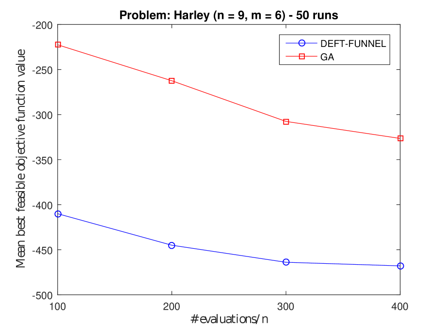


Figure 5 shows the results on test problems SR7, Hesse, Gómez #3 and G3. DEFT-FUNNEL and GA had similar performances on SR7, Hesse and G3 problems, while PS had the poorest performance. GA was the best method on Gómez #3, being very close to the global minimum in the end. Finally, PS performance on SR7 shows that allowing more black-box calls was not helpful and that the objective function value even increased.
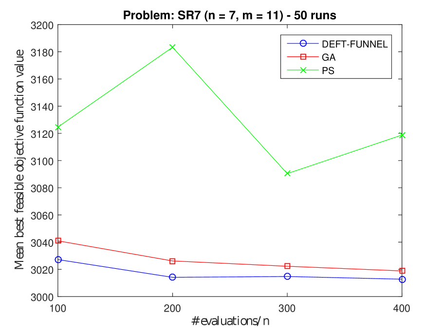


Figure 6 shows the results on test problems G4, G6, G7, G8, G9 and G11. DEFT-FUNNEL was superior to all other methods, attaining global optimality on 4 problems independently of the number of evaluations allowed. GA was the second best, followed by PS. Besides that PS did not find a feasible solution on Harley pooling problem, there is a significant increase on its objective function value as the number of evaluations grows on test problems SR7 and G7. These 3 problems are the ones with the largest number of constraints, which could be a reason for its poor performance.


4.2 Grey-box optimization problems
In this section, DEFT-FUNNEL is compared with GA and PS on a set of artificial grey-box problems built by selecting a test problem and defining some of its functions as black boxes and the remaining as white boxes. Among the 5 grey-box problems considered in the experiments, 3 were used in the black-box experiments described in the previous subsection, where all functions were considered as black boxes, namely: Hesse, SR7 and GTCD4. The reuse of these test problems allows for evaluating the performance improvement of DEFT-FUNNEL in cases where some information is available and for comparing its performance with that obtained in the black-box setting. The remaining grey-box problems are the problems 21 and 23 from the well-known Hock-Schittkowski collection [24], denoted here as HS21 and HS23, respectively. Both HS21 and HS23 have nonlinear objective functions; however, in HS21 the objective function is defined as white box, while in HS23 it is defined is black box. The only constraint present in HS21 is defined as black box, while in HS23 there is a balance between both categories among the constraints. We have therefore attempted to cover different possibilities related to the type of functions in a grey-box setting. The derivatives of all functions defined as white boxes were given as input to DEFT-FUNNEL. The reader can find more details about the tested grey-box problems in Table 5.
| Test problem | Number of | Number of | Number of | Type of | Best known feasible |
| variables | BB constraints | WB constraints | Obj. function | obj. function value | |
| GTCD4 | 4 | 0 | 1 | BB | 2964893.85 |
| SR7 | 7 | 9 | 2 | WB | 2994.42 |
| Hesse | 6 | 3 | 3 | WB | -310 |
| HS21 | 2 | 1 | 0 | WB | -99.96 |
| HS23 | 2 | 3 | 2 | WB | 2 |
In Table 6, the results obtained with a budget of 100 black-box calls are presented. It can be seen that DEFT-FUNNEL was the only one to reach the global minimum in every problem, while GA had the best average-case and worst-case performances in general. We also notice that the three solvers had similar performances on HS21, attaining all the global minimum without much difficulty.
When comparing the black-box and grey-box results obtained by DEFT-FUNNEL on problems GTCD4 and SR7, it is evident that the available information from the white-box functions contributed to improve its performance. Not only the best objective function values on these problems were improved, allowing for reaching the global minimum on SR7, but also the average and worst ones. Since DEFT-FUNNEL had already attained the global minimum on Hesse in the black-box setting, the only expected improvement would be in the average and worst cases, which did not happen in our experiments. This is probably due to the fact that this a multimodal problem with 18 local minima, being a combination of 3 separable problems and having 1 global minimum. Therefore, even if information about the function is partially available, the problem remains very difficult to solve due to its nature.
| Prob | Solver | Best | Avg. | Worst | |
|---|---|---|---|---|---|
| GTCD4 | 2964893.85 | GA | 4004353.4045 | 9693274.3280 | 13860176.1776 |
| PS | 4953046.0849 | 12212940.1950 | 13786675.7772 | ||
| DEFT-FUNNEL | 3564559.7818 | 9994027.4513 | 13937534.7346 | ||
| SR7 | 2994.42 | GA | 3027.8978 | 3151.6054 | 3438.7069 |
| PS | 3134.0525 | 3516.1761 | 5677.6224 | ||
| DEFT-FUNNEL | 2994.4244 | 3370.8758 | 4274.8433 | ||
| Hesse | -310 | GA | -292.1091 | -277.1073 | -259.1020 |
| PS | -302.1163 | -162.5650 | -49.4364 | ||
| DEFT-FUNNEL | -310 | -210.6784 | -36 | ||
| HS21 | -99.96 | GA | -99.9599 | -99.5528 | -95.6688 |
| PS | -99.9599 | -99.9435 | -99.8086 | ||
| DEFT-FUNNEL | -99.96 | -99.9593 | -99.9267 | ||
| HS23 | 2 | GA | 4.7868 | 13.7529 | 174.1049 |
| PS | 4.5138 | 45.6059 | 274.6368 | ||
| DEFT-FUNNEL | 2 | 424.9427 | 1242.011 |
5 Conclusions
We have introduced a new global optimization solver for general constrained grey-box and black-box optimization problems named DEFT-FUNNEL. It combines a stochastic multistart strategy with a trust-funnel sequential quadratic optimization algorithm where the black-box functions are replaced by surrogate models built from polynomial interpolation. The proposed solver is able to exploit available information from white-box functions rather than considering them as black boxes. Its code is open source and freely available at the Github repository http://github.com/phrsampaio/deft-funnel. Unlike many black-box optimization algorithms, it can handle both inequality and equality constraints and it does not require feasible starting points. Moreover, the constraints are treated individually rather than grouped into a penalty function.
We have shown that DEFT-FUNNEL compares favourably with other state-of-the-art algorithms available for the optimization community on a collection of well-known benchmark problems. The reported numerical results indicate that the proposed approach is very promising for grey-box and black-box optimization. Future research works include extensions for multiobjective optimization and mixed-integer nonlinear optimization as well as as parallel version of the solver.
References
- Amaioua et al. [2018] N. Amaioua, C. Audet, A. R. Conn, and S. L. Digabel. Efficient solution of quadratically constrained quadratic subproblems within the mesh adaptive direct search algorithm. European Journal of Operational Research, 268(1):13–24, 2018. ISSN 0377-2217. doi: https://doi.org/10.1016/j.ejor.2017.10.058. URL http://www.sciencedirect.com/science/article/pii/S0377221717309876.
- Armstrong and Favorite [2016] J. C. Armstrong and J. A. Favorite. Using a derivative-free optimization method for multiple solutions of inverse transport problems. Optimization and Engineering, 17(1):105–125, Mar 2016. ISSN 1573-2924. doi: 10.1007/s11081-015-9306-x. URL https://doi.org/10.1007/s11081-015-9306-x.
- Audet and Dennis [2006] C. Audet and J. Dennis. Mesh adaptive direct search algorithms for constrained optimization. SIAM Journal on Optimization, 17(1):188–217, 2006. doi: 10.1137/040603371. URL https://doi.org/10.1137/040603371.
- Audet and Hare [2017] C. Audet and W. Hare. Derivative-Free and Blackbox Optimization. Springer, Cham, 2017. ISBN 978-3-319-68912-8. doi: https://doi.org/10.1007/978-3-319-68913-5.
- Audet et al. [2015] C. Audet, S. L. Digabel, and M. Peyrega. Linear equalities in blackbox optimization. Computational Optimization and Applications, 61(1):1–23, May 2015. ISSN 1573-2894. doi: 10.1007/s10589-014-9708-2. URL https://doi.org/10.1007/s10589-014-9708-2.
- Bajaj et al. [2018] I. Bajaj, S. S. Iyer, and M. M. F. Hasan. A trust region-based two phase algorithm for constrained black-box and grey-box optimization with infeasible initial point. Computers & Chemical Engineering, 116:306–321, 2018. ISSN 0098-1354. doi: https://doi.org/10.1016/j.compchemeng.2017.12.011. URL http://www.sciencedirect.com/science/article/pii/S0098135417304404.
- Beightler and Phillips [1976] C. S. Beightler and D. T. Phillips. Applied Geometric Programming. John Wiley & Sons Inc, New York, 1976.
- Birgin et al. [2000] E. G. Birgin, J. M. Martínez, and M. Raydan. Nonmonotone spectral projected gradient methods on convex sets. SIAM Journal on Optimization, 10(4):1196–1211, 2000.
- Boukouvala et al. [2017] F. Boukouvala, M. M. F. Hasan, and C. A. Floudas. Global optimization of general constrained grey-box models: new method and its application to constrained pdes for pressure swing adsorption. Journal of Global Optimization, 67(1):3–42, Jan 2017. ISSN 1573-2916. doi: 10.1007/s10898-015-0376-2. URL https://doi.org/10.1007/s10898-015-0376-2.
- Bueno et al. [2013] L. Bueno, A. Friedlander, J. Martínez, and F. Sobral. Inexact restoration method for derivative-free optimization with smooth constraints. SIAM Journal on Optimization, 23(2):1189–1213, 2013. doi: 10.1137/110856253. URL https://doi.org/10.1137/110856253.
- Coello and Montes [2002] C. A. C. Coello and E. M. Montes. Constraint-handling in genetic algorithms through the use of dominance-based tournament selection. Advanced Engineering Informatics, 16(3):193–203, 2002. ISSN 1474–0346. doi: https://doi.org/10.1016/S1474-0346(02)00011-3. URL http://www.sciencedirect.com/science/article/pii/S1474034602000113.
- Conn et al. [2009] A. R. Conn, K. Scheinberg, and L. N. Vicente. Introduction to derivative-free optimization. MPS-SIAM Book Series on Optimization, Philadelphia, 2009.
- Deb [2000] K. Deb. An efficient constraint handling method for genetic algorithms. Computer Methods in Applied Mechanics and Engineering, 186(2):311 – 338, 2000. ISSN 0045-7825. doi: https://doi.org/10.1016/S0045-7825(99)00389-8. URL http://www.sciencedirect.com/science/article/pii/S0045782599003898.
- Echebest et al. [2017] N. Echebest, M. L. Schuverdt, and R. P. Vignau. An inexact restoration derivative-free filter method for nonlinear programming. Computational and Applied Mathematics, 36(1):693–718, Mar 2017. ISSN 1807-0302. doi: 10.1007/s40314-015-0253-0. URL https://doi.org/10.1007/s40314-015-0253-0.
- Floudas [2000] C. Floudas. Deterministic Global Optimization: Theory, Methods and Applications. Springer, Boston, MA, 2000. ISBN 978-1-4419-4820-5. doi: https://doi.org/10.1007/978-1-4757-4949-6.
- Floudas et al. [1999] C. Floudas, P. Pardalos, C. Adjiman, W. R. Esposito, Z. H. Gümüs, S. T. Harding, J. L. Klepeis, C. A. Meyer, and C. A. Schweiger. Handbook of Test Problems in Local and Global Optimization. Springer US, 1999. ISBN 978-0-7923-5801-5. doi: 10.1007/978-1-4757-3040-1.
- Floudas and Pardalos [1990] C. A. Floudas and P. M. Pardalos. A Collection of Test Problems for Constrained Global Optimization Algorithms. Springer-Verlag, Berlin, Heidelberg, 1990. ISBN 0-387-53032-0.
- Gómez and Levy [1982] S. Gómez and A. V. Levy. The tunnelling method for solving the constrained global optimization problem with several non-connected feasible regions. In J. P. Hennart, editor, Numerical Analysis, pages 34–47, Berlin, Heidelberg, 1982. Springer Berlin Heidelberg. ISBN 978-3-540-38986-6.
- Gould and Toint [2010] N. I. M. Gould and P. L. Toint. Nonlinear programming without a penalty function or a filter. Mathematical Programming, 122(1):155–196, Mar 2010. ISSN 1436-4646. doi: 10.1007/s10107-008-0244-7. URL https://doi.org/10.1007/s10107-008-0244-7.
- Gratton et al. [2011] S. Gratton, P. L. Toint, and A. Tröltzsch. An active-set trust-region method for bound-constrained nonlinear optimization without derivatives. Optimization Methods and Software, 26(4-5):875–896, 2011.
- Griewank [2003] A. Griewank. A mathematical view of automatic differentiation. Acta Numerica, 12:321––398, 2003. doi: 10.1017/S0962492902000132.
- Griewank and Walther [2008] A. Griewank and A. Walther. Evaluating Derivatives. Society for Industrial and Applied Mathematics, second edition, 2008. doi: 10.1137/1.9780898717761. URL https://epubs.siam.org/doi/abs/10.1137/1.9780898717761.
- Hesse [1973] R. Hesse. A heuristic search procedure for estimating a global solution of nonconvex programming problems. Operations Research, 21(6):1267–1280, 1973. doi: 10.1287/opre.21.6.1267. URL https://doi.org/10.1287/opre.21.6.1267.
- Hock and Schittkowski [1980] W. Hock and K. Schittkowski. Test examples for nonlinear programming codes. Journal of Optimization Theory and Applications, 30(1):127–129, 1980. doi: 10.1007/BF00934594. URL https://doi.org/10.1007/BF00934594.
- Jones et al. [1998] D. R. Jones, M. Schonlau, and W. J. Welch. Efficient global optimization of expensive black-box functions. Journal of Global Optimization, 13(4):455–492, Dec 1998. ISSN 1573-2916. doi: 10.1023/A:1008306431147. URL https://doi.org/10.1023/A:1008306431147.
- Kan and Timmer [1987a] A. H. G. R. Kan and G. T. Timmer. Stochastic global optimization methods part i: Clustering methods. Mathematical Programming, 39(1):27–56, Sep 1987a. ISSN 1436-4646. doi: 10.1007/BF02592070. URL https://doi.org/10.1007/BF02592070.
- Kan and Timmer [1987b] A. H. G. R. Kan and G. T. Timmer. Stochastic global optimization methods part ii: Multi level methods. Mathematical Programming, 39(1):57–78, Sep 1987b. ISSN 1436-4646. doi: 10.1007/BF02592071. URL https://doi.org/10.1007/BF02592071.
- Larson et al. [2019] J. Larson, M. Menickelly, and S. M. Wild. Derivative-free optimization methods. Acta Numerica, 28:287–404, 2019. doi: 10.1017/S0962492919000060.
- Lewis and Torczon [2002] R. Lewis and V. Torczon. A globally convergent augmented lagrangian pattern search algorithm for optimization with general constraints and simple bounds. SIAM Journal on Optimization, 12(4):1075–1089, 2002. doi: 10.1137/S1052623498339727. URL https://doi.org/10.1137/S1052623498339727.
- Locatelli [1998] M. Locatelli. Relaxing the assumptions of the multilevel single linkage algorithm. Journal of Global Optimization, 13(1):25–42, Jan 1998. ISSN 1573-2916. doi: 10.1023/A:1008246031222. URL https://doi.org/10.1023/A:1008246031222.
- Maratos [1978] N. Maratos. Exact penalty function algorithms for finite dimensional and control optimization problems. Department of Control Theory, Imperial College London, 1978. URL https://books.google.fr/books?id=Ar2AtgAACAAJ.
- MATLAB [2015] MATLAB. 2015b. The MathWorks Inc., Natick, Massachusetts, 2015.
- McKay et al. [1979] M. D. McKay, R. J. Beckman, and W. J. Conover. A comparison of three methods for selecting values of input variables in the analysis of output from a computer code. Technometrics, 21(2):239–245, 1979. ISSN 00401706. URL http://www.jstor.org/stable/1268522.
- Michalewicz and Schoenauer [1996] Z. Michalewicz and M. Schoenauer. Evolutionary algorithms for constrained parameter optimization problems. Evolutionary Computation, 4(1):1–32, March 1996. doi: 10.1162/evco.1996.4.1.1.
- Nocedal and Wright [2006] J. Nocedal and S. J. Wright. Numerical optimization. Springer Series in Operations Research and Financial Engineering. Springer, New York, NY, 2. ed. edition, 2006. ISBN 978-0-387-30303-1.
- Powell [1994] M. J. D. Powell. A direct search optimization method that models the objective and constraint functions by linear interpolation. In S. Gomez and J.-P. Hennart, editors, Advances in Optimization and Numerical Analysis, pages 51–67. Springer Netherlands, Dordrecht, 1994. ISBN 978-94-015-8330-5. doi: 10.1007/978-94-015-8330-5_4. URL https://doi.org/10.1007/978-94-015-8330-5_4.
- Regis [2011] R. G. Regis. Stochastic radial basis function algorithms for large-scale optimization involving expensive black-box objective and constraint functions. Computers & Operations Research, 38(5):837–853, 2011. ISSN 0305-0548. doi: https://doi.org/10.1016/j.cor.2010.09.013. URL http://www.sciencedirect.com/science/article/pii/S030505481000208X.
- Regis [2014] R. G. Regis. Constrained optimization by radial basis function interpolation for high-dimensional expensive black-box problems with infeasible initial points. Engineering Optimization, 46(2):218–243, 2014. doi: 10.1080/0305215X.2013.765000. URL https://doi.org/10.1080/0305215X.2013.765000.
- Regis and Shoemaker [2005] R. G. Regis and C. A. Shoemaker. Constrained global optimization of expensive black box functions using radial basis functions. Journal of Global Optimization, 31(1):153–171, Jan 2005. ISSN 1573-2916. doi: 10.1007/s10898-004-0570-0. URL https://doi.org/10.1007/s10898-004-0570-0.
- Regis and Shoemaker [2007] R. G. Regis and C. A. Shoemaker. A stochastic radial basis function method for the global optimization of expensive functions. INFORMS Journal on Computing, 19(4):497–509, 2007. doi: 10.1287/ijoc.1060.0182. URL https://doi.org/10.1287/ijoc.1060.0182.
- Rios and Sahinidis [2013] L. M. Rios and N. V. Sahinidis. Derivative-free optimization: a review of algorithms and comparison of software implementations. Journal of Global Optimization, 56(3):1247–1293, Jul 2013. ISSN 1573-2916. doi: 10.1007/s10898-012-9951-y. URL https://doi.org/10.1007/s10898-012-9951-y.
- Sampaio and Toint [2015] P. R. Sampaio and P. L. Toint. A derivative-free trust-funnel method for equality-constrained nonlinear optimization. Computational Optimization and Applications, 61(1):25–49, May 2015. ISSN 1573-2894. doi: 10.1007/s10589-014-9715-3. URL https://doi.org/10.1007/s10589-014-9715-3.
- Sampaio and Toint [2016] P. R. Sampaio and P. L. Toint. Numerical experience with a derivative-free trust-funnel method for nonlinear optimization problems with general nonlinear constraints. Optimization Methods and Software, 31(3):511–534, 2016. doi: 10.1080/10556788.2015.1135919. URL https://doi.org/10.1080/10556788.2015.1135919.
- Scheinberg and Toint [2010] K. Scheinberg and P. L. Toint. Self-correcting geometry in model-based algorithms for derivative-free unconstrained optimization. SIAM Journal on Optimization, 20(6):3512–3532, 2010.
- Sendín et al. [2009] J.-O. H. Sendín, J. R. Banga, and T. Csendes. Extensions of a multistart clustering algorithm for constrained global optimization problems. Industrial & Engineering Chemistry Research, 48(6):3014–3023, 2009. doi: 10.1021/ie800319m. URL https://doi.org/10.1021/ie800319m.
- Zhang et al. [2010] H. Zhang, A. Conn, and K. Scheinberg. A derivative-free algorithm for least-squares minimization. SIAM Journal on Optimization, 20(6):3555–3576, 2010. doi: 10.1137/09075531X. URL https://doi.org/10.1137/09075531X.