Deformation and dewetting of liquid films under gas jets

A schematic representation of the model system is shown in figure 3. We denote the radius of the beaker by $R_{b}$ and its height by $H$. The thickness of the undisturbed liquid layer is denoted by $h_{0}$. The inner and outer radii of the nozzle are denoted by $R_{i}$ and $R_{o}$, respectively, and the distance between the nozzle and the undisturbed gas–liquid interface is denoted by $h_{1}$. We introduce cylindrical polar coordinates $(R,\varphi,z)$ with the $z$-axis pointing upwards along the axis of the beaker in the direction opposite to gravity $\boldsymbol{g}$, and with the bottom of the beaker coinciding with the $z=0$ plane. The deformed gas–liquid interface is denoted by $\Sigma$ and is given by the equation ${f(R,\varphi,z,t)=0}$. In the simplest case, the interface is given by the graph of a function, $z=h(R,\varphi,t)$, and hence $f=h-z$. We assume that the liquid and the gas are of the same constant temperature.

As the gas jet strikes the liquid surface at the centre, the surface of the liquid deforms and a cavity appears. Motion in the liquid, in the form of eddies is also generated. The eddies affect the mass transfer and mixing in the liquid. In order to describe such a system, the Navier–Stokes and continuity equations are used and the corresponding boundary conditions must be satisfied.

As the typical velocity in the liquid will be assumed to be small compared to the speed of sound in the liquid, it is appropriate to model the liquid problem by the incompressible Navier–Stokes equations:

where $\rho_{l}$ is the liquid density, which is assumed to be constant, $\boldsymbol{u}$ is the velocity field in the liquid, $D/Dt={\partial}/{\partial t}+\boldsymbol{u}\cdot\nabla$ is the usual material derivative, and $\boldsymbol{\sigma}_{l}$ is the viscous stress tensor for the liquid given by

where $p_{l}$ is the pressure in the liquid, $\mu_{l}$ is the viscosity of the liquid, which is assumed to be constant, $\boldsymbol{\delta}$ is the identity tensor and $\boldsymbol{S}_{l}=\frac{1}{2}\bigl{[}(\nabla\boldsymbol{u})^{T}+\nabla\boldsymbol{u}\bigr{]}$ is the strain-rate tensor.

In the present study, we consider gas velocities up to $50\,\mathrm{m}/\mathrm{s}$. For such gas velocities, compressibility effects may also be neglected in the gas phase. For such gas velocities it is still appropriate to assume that the gas flow is laminar. The incompressible Navier–Stokes equations in the gas then take the form

where $\rho_{g}$ is the gas density, $\boldsymbol{v}$ is the gas velocity and $\boldsymbol{\sigma}_{g}$ is the viscous stress tensor for the gas given by

where $p_{g}$ is the gas pressure, $\mu_{g}$ is the viscosity of the gas, which is assumed to be constant, and $\boldsymbol{S}_{g}=\frac{1}{2}\bigl{[}(\nabla\boldsymbol{v})^{T}+\nabla\boldsymbol{v}\bigr{]}$ is the strain-rate tensor in the gas.

We impose no-slip and no-penetration conditions both for the liquid and for the gas at the solid boundaries ($\boldsymbol{u}=\boldsymbol{0}$ and $\boldsymbol{v}=\boldsymbol{0}$) except at the beaker side wall, where no-penetration still applies, but instead of no-slip, we impose the Navier slip condition to allow for the motion of the contact line (see, e.g., Sibley et al., 2012). So for the liquid when $R=R_{b}$ we have

where $\hat{\boldsymbol{n}}_{w}$ is a unit normal vector to the side wall pointing into the beaker (i.e. $\hat{\boldsymbol{n}}_{w}=-\hat{\boldsymbol{R}}$, where $\hat{\boldsymbol{R}}$ is a unit vector pointing in the $R$ direction), $\hat{\boldsymbol{t}}_{w}$ is a unit tangent vector to the wall, $\beta_{NS}^{l}$ is the slip coefficient for the liquid. For the gas when $R=R_{b}$ we have

where $\beta_{NS}^{g}$ is the slip coefficient for the gas.

Note that in (5) and (6), there are, in general, two independent tangent directions to the wall, i.e. each of the equations results in two scalar equations, by taking $\hat{\boldsymbol{t}}_{w}=\hat{\boldsymbol{k}}$ and $\hat{\boldsymbol{t}}_{w}=\hat{\boldsymbol{\varphi}}$, where $\hat{\boldsymbol{k}}$ and $\hat{\boldsymbol{\varphi}}$ are unit vectors pointing in the $z$ and $\varphi$ directions. However, we will later assume axisymmetry, i.e. no dependence on $\varphi$, and then it will be sufficient to only consider $\hat{\boldsymbol{t}}_{w}=\hat{\boldsymbol{k}}$.

In addition, we impose a fixed contact angle condition at the contact line, so that when the interface is given by $z=h(R,\varphi,t)$, we have

when $R=R_{b}$ and $z=h(R_{b},\varphi,t)$, where $\theta_{c}$ is the angle the liquid makes with the wall at the contact line.

In a subset of our numerical simulations presented below, at the bottom of the beaker we also impose the Navier slip condition instead of the no-slip condition. This allows us to study dewetting induced by the gas jet using DNS where topological transitions of the gas–liquid interface are allowed. We do this with the volume-of-fluid package $\mathpzc{Gerris}$ (e.g. Popinet, 2009), as will be explained below. The contact angle at the bottom of the beaker will be denoted by $\theta_{eq}$. We also performed DNS in the CFD finite-element package COMSOL (e.g. Pryor, 2011), and our implementation allows for mesh movements so that the mesh deformations follow the gas–liquid interface motion. Such an implementation allows us to analyse the deformations of the interface very accurately but forbids topological transitions.

At the gas inlet, when $z=h_{0}+h_{1}$ and $0\leq R\leq R_{i}$, we impose the fully developed laminar Poiseuille velocity profile:

where $v_{\mathrm{max}}=2q_{g}/\pi R_{i}^{2}$, with $q_{g}$ denoting the imposed gas flow rate.

At the gas outlet, when $z=H$ and $R_{o}<R<R_{b}$, we impose normal flow, and prescribe normal stress, i.e. we require $\hat{\boldsymbol{k}}\cdot\boldsymbol{\sigma}_{g}\cdot\hat{\boldsymbol{k}}=-p_{a}$, where $p_{a}$ is the atmospheric pressure.

Finally, we discuss conditions that must be satisfied at the gas–liquid interface $\Sigma$. First, we have the kinematic condition

where we remind that $f$ is a function such that $\Sigma$ is given by the equation ${f(R,\varphi,z,t)=0}$. Continuity of velocity must also be satisfied at the interface, $\boldsymbol{u}=\boldsymbol{v}$, and we must have dynamic balance of stress at $\Sigma$:

Here, $\hat{\boldsymbol{n}}$ is the unit normal vector to the interface pointing into the liquid. The term on the right-hand side is due to the Laplace pressure, where $\gamma$ is the gas–liquid surface tension coefficient (which is assumed to be constant) and $\kappa=\nabla\cdot\hat{\boldsymbol{n}}$ is twice the mean curvature of the interface $\Sigma$.

Note that to study dewetting induced by the gas jet in a numerical formulation where topological transitions are not allowed, we also include a Derjaguin (or disjoining) pressure in the stress balance condition. This approach is applicable when $\Sigma$ is a graph of a function, $z=h(R,\varphi,t)$. The stress balance condition then becomes

The disjoining pressure represents an effective interaction between the gas–liquid interface and the liquid–substrate interface. It can be written as $\Pi(h)=-\mathrm{d}V(h)/dh$, where $V(h)$ is the so-called binding potential (e.g. de Gennes et al., 2013). The disjoining pressure is assumed to be of the form (e.g. Pismen, 2002; Galvagno et al., 2014)

where the first term results from the long-range attractive forces (with $A$ representing the Hamaker constant) and the second term results from the short-range repulsive forces. The second term prevents the liquid film from breaking down, and instead of this occurring we obtain a very thin precursor film. In practice, where the film thickness is equal to the thickness of the precursor film, we may assume that a dry spot has appeared. At equilibrium, the thickness of the precursor film corresponds to the minimum of the binding potential $V(h)$ and is equal to

with the contact angle at the apparent contact line is given by (e.g. Rauscher & Dietrich, 2008; Hughes et al., 2015)

Note that given the precursor thickness, $h_{eq}$, and the equilibrium contact angle, $\theta_{eq}$, the constants $A$ and $B$ can be recovered using relations (13) and (14) given above.

Solving the full system of governing equations is a computationally expensive task. We therefore aim to simplify the problem by deriving an accurate reduced-order model. Such a model not only provides insight into the fundamental features of the system in an efficient way but also serves as a mechanism to guide the more computationally prohibitive DNS tools towards suitable regimes with a much more informed view of an otherwise vast parameter space. The first step is to decouple the problem for the gas from that for the liquid, which is possible when the typical velocity in the liquid is much smaller than that in the gas. Then, for the gas problem it is appropriate to neglect the motion of the liquid and to use the quasi-static assumption, i.e. it is appropriate to model the interface as a rigid wall and solve the gas problem independently, see e.g. Tuck (1975) who states that such an assumption is appropriate when the typical liquid velocity is less than approximately $4\%$ of the typical gas velocity, which is always the case in our study (see also Tseluiko & Kalliadasis, 2011; Vellingiri et al., 2015, for more recent studies, where the quasi-static assumption was used in the modelling of a liquid film sheared by a turbulent gas).

The solution of the gas problem can then be used to obtain the stress exerted by the gas onto the gas–liquid interface, which can then be fed into the normal and tangential stress balance conditions at the interface. We denote such a stress by $\boldsymbol{s}_{g}$ so that

For the analysis in this section, we first consider the general non-axisymmetric case, and for convenience we use Cartesian coordinates $(x,y,z)$ (so that the $z$ direction remains as before.

We non-dimensionalise the equations using $h_{0}$ as the length scale, $U_{0}$ as the velocity scale (to be specified later), $h_{0}/U_{0}$ as the time scale and $\mu_{l}U_{0}/h_{0}$ as the scale for pressure and the gas stress, so from now on all the variables will be assumed to be dimensionless. We thus introduce dimensionless variables via the following mappings:

where we denote by $u$, $v$ and $w$ the $x$, $y$ and $z$ components of the velocity, respectively.

The incompressible Navier–Stokes and continuity equations in the liquid become

where $Re$ and $G$ are the Reynolds and the gravity numbers, respectively, given by

The no-slip and no-penetration conditions at the bottom of the beaker become

The kinematic condition at the interface, $z=h(x,y,t)$, takes the form

The normal stress balance condition takes the form:

at $z=h(x,y,t)$, where $Ca$ is the Capillary number given by

$N_{s}$ is the dimensionless normal stress exerted by the gas on the gas–liquid interface

which under the quasi-static assumption can be assumed to be a functional of the interface shape, $N_{s}=N_{s}[h]$, and finally, $\overline{\Pi}(h)$ is the dimensionless disjoining pressure, given by

where $\overline{A}=A/\mu_{l}U_{0}h_{0}^{2}$ and $\overline{B}=B/\mu_{l}U_{0}h_{0}^{5}$.

Taking $\hat{\boldsymbol{t}}=\hat{\boldsymbol{t}}_{1}={(1,0,h_{x})}/{\sqrt{1+h_{x}^{2}}}$ and $\hat{\boldsymbol{t}}=\hat{\boldsymbol{t}}_{2}={(0,1,h_{y})}/{\sqrt{1+h_{y}^{2}}}$ in the tangential stress balance condition, we obtain

at $z=h(x,y,t)$, where $T_{si}$, $i=1,2$, are the $\hat{\boldsymbol{t}}_{1}$ and $\hat{\boldsymbol{t}}_{2}$ components of the tangential stress exerted by the gas on the gas–liquid interface, $T_{si}=\boldsymbol{s}_{g}\cdot\hat{\boldsymbol{t}_{i}}$, which under the quasi-static assumption can be assumed to be functionals of the interface shape, $T_{si}=T_{si}[h]$. The tangential stress exerted by the gas on the gas–liquid interface is then expressed as

Next, we utilise the so-called thin-film or long-wave approximation, namely, we assume that the undisturbed film thickness, $h_{0}$, is much smaller than the characteristic horizontal length scale $\ell$ over which variations in the film thickness occur, and we introduce the so-called thin-film parameter $\epsilon=h_{0}/\ell\ll 1$. We now use the following additional rescalings of variables that are standard for the thin-film approximation:

To derive the thin-film equation, we consider the asymptotic limit $\epsilon\rightarrow 0$. Then, to keep capillary effects at leading order, we assume that $Ca$ is asymptotically bounded above and below by $\epsilon^{3}$. To neglect inertia at leading order, we assume that $Re\ll 1/\epsilon$. We also assume that $G=O(1/\epsilon)$, so that gravitational effects may enter at leading order. For the disjoining pressure, it is appropriate to assume that $\overline{\Pi}=O(1/\epsilon)$. In addition, for the dimensionless gas stress, we need to assume that $N_{s}=O(1/\epsilon)$ and $T_{si}=O(1)$, $i=1,2$. We then introduce the following rescaled parameters:

so that $\widetilde{C}a$ is asymptotically bounded above and below by non-zero constants and $\widetilde{G}=O(1)$, and the following rescaled gas normal stress:

so that $\widetilde{N}_{s}=O(1)$, and the rescaled disjoining pressure:

so that $\widetilde{\Pi}=O(1)$.

The problem at leading order becomes:

with the no-slip and no-penetration conditions

at $z=0$ and the tangential and normal stress balances

at $z=h(\xi,\eta,\tau)$. We also have the kinematic condition, which can be rewritten as

where $\nabla=(\partial/\partial\xi,\partial/\partial\eta)$ and

is the flux vector parallel to the plane $z=0$.

Then we find that the pressure at leading order is given by

and the velocity components at leading order are given by

Substituting the leading-order expressions for $u$ and $v$ into the expression for the flux vector (40), we find that at leading order

Substituting this expression into the kinematic condition (39) gives the following evolution equation for the film thickness, the so-called thin-film equation:

Scaling back to the dimensionless variables $x$, $y$ and $t$, we obtain

where the dimensionless leading-order pressure is given by

and $\nabla=(\partial/\partial x,\partial/\partial y)$.

For convenience, it is possible to eliminate one of the dimensionless parameters by, for example, multiplying the thin-film equation by $Ca$ and appropriately rescaling time. This is equivalent to choosing $U_{0}=\gamma/\mu_{l}$, for which the time scale becomes $\mu_{l}h_{0}/\gamma$ and the scale for pressure and the gas stress becomes $\gamma/h_{0}$. Then the pressure in the thin-film equation takes the form

where $Bo$ is the Bond number given by

and the dimensionless coefficients in the disjoining pressure are $\overline{A}=A/\gamma h_{0}^{2}$ and $\overline{B}=B/\gamma h_{0}^{5}$.

For the validity of the thin-film equation in terms of dimensionless parameters that are independent of $U_{0}$, we must have $Bo=O(\epsilon^{2})$ and $La\ll 1/\epsilon^{4}$, where $La$ is the Laplace number given by

The latter condition is needed for inertia to be negligible. We must additionally have $N_{s}=O(\epsilon^{2})$ and $T_{si}=O(\epsilon^{3})$, $i=1,2$. The validity of the thin-film equation for the experimental parameter values that we have used is discussed § 4.

Finally, going back to cylindrical polar coordinates $(R,\varphi,z)$ and assuming axisymmetry, we obtain the following equation:

where $T_{s}$ denotes the gas tangential stress in the $R$-direction and pressure is given by

Note that here $R$ is assumed to be non-dimensionalised using $h_{0}$ as the length scale. To solve the thin-film equation (51) numerically, we also need to impose appropriate boundary conditions. Conditions at $R=0$ follow from the symmetry assumption:

At the side wall, we will assume for simplicity that the contact angle is $90^{\circ}$, so that

where $\overline{R}_{b}=R_{b}/h_{0}$, and we will impose zero flux in the $R$ direction, so that

For analysing flow patterns in the liquid film, it is also useful to give the $R$ and $z$ velocity components in cylindrical polar coordinates:

Note that the main model equation (51) provides a highly efficient route towards studying mechanistic aspects of the flow and generating an understanding of the underlying physics, thus forming a valuable part of our methodology toolkit.

To close the thin-film model, we need to specify stress contributions $N_{s}$ and $T_{s}$. There are different possible approaches for incorporating these. As mentioned in the introduction, often approximate expressions for these stresses were used that were typically constructed on the basis of general unbounded domains. For example, Kriegsmann et al. (1998) and Lunz & Howell (2018) assumed a Gaussian form for the normal stress and completely ignored the shear stress. We choose to integrate the gas effects into the the thin-film equation more carefully by means of exploiting detailed knowledge of the flow field in the gas extracted from DNS. In the first instance and for comparison purposes, we suggest computationally informed functional expressions for $N_{s}$ and $T_{s}$, thus developing an accurate “one-sided” model. However, more generally, we also introduce and utilise an iterative numerical procedure for computing $N_{s}$ and $T_{s}$, which provides an accurate update mechanism that is computationally inexpensive and powerful in the context of predictive modelling, especially in the context of finite-size effects generated by the presence of the lateral walls of the beaker.

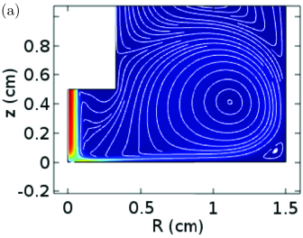
First, we discuss the decoupled gas problem and explain how the gas normal and tangential stresses exerted on the interface are computed using an iterative procedure. Under the quasi-static assumption, we model the liquid surface as a solid wall obtaining a problem for the gas only, and initially we assume that the interface is flat. The gas flow rapidly develops into a steady state. The resulting gas flow pattern at steady state obtained using COMSOL is shown in figure 4(a) for the gas flow rate $q_{g}=1\,\mathrm{slpm}$, which corresponds to the maximum gas speed of approximately $16\,\mathrm{m}\,\mathrm{s}^{-1}$. In this section, we assume that the undisturbed interface is located at $z=0$. We note that $\mathpzc{Gerris}$ simulations agree with the COMSOL results. The colour scheme indicates the gas speed in metres per second and the thin white lines show streamlines. We can observe that the gas jet impinges onto the lower wall, and then the gas flows in the direction parallel to the wall radially outwards with its speed decreasing as the radial distance increases. We can also observe that a relatively large recirculation zone (eddy) is generated in the gas, and there is also a small, relatively slow eddy in the bottom-right corner. This solution of the gas problem for the interface modelled as a flat solid wall is used to compute the normal and tangential stresses exerted by the gas jet on the interface at different radial locations. Next, we use these stresses in the thin-film equation (51) to solve the problem for the liquid film and therefore obtain the deformation of the interface resulting from these stresses. The thin-film equation is solved numerically in Matlab using finite-difference approximations for the spatial derivatives and Matlab’s ode15s solver for stepping in time. For this gas flow rate, the solution evolves into a steady state within a few seconds. An example of a deformed interface computed in this way is shown in figure 4(b). A liquid film of thickness $5\,\mathrm{mm}$ was used for illustrative purposes (although we note that the thin-film equation is not expected to be valid for such a thickness). Next, we use this deformed interface as the lower boundary for the gas domain and again assume that it is a solid wall and recompute the solution of the decoupled gas problem. It can be seen in figure 4(b) that the computed solution is qualitatively similar to the one in figure 4(a). We extract the gas stresses from this solutions and use these updated stresses to solve the thin-film equation again to obtain an updated steady-stated interface shape. This procedure is repeated until a converged steady-state interface shape is achieved. Typically, we find that for the relatively thin films considered in the present study 2–3 iterations are sufficient to obtain a converged profile to within graphical accuracy. It is expected that for thicker liquid films and stronger interfacial deformations more iterations might be needed. Other fluid systems with properties further away from the present modelling assumptions are also anticipated to give rise to a more challenging convergence procedure.

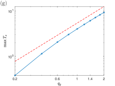
Next, we will analyse in detail how the normal and tangential stresses exerted by the gas onto the interface behave when the gas flow rate varies for the case when the interface is modelled as a flat solid wall. The results are presented in figure 5. Panels (a) and (e) show the normal and tangential stresses for the gas flow rate $q_{g}$ changing from $0.2$ (red dashed lines) to $2\,\mathrm{slpm}$ (thick blue solid lines) with the increment of $0.2\,\mathrm{slpm}$. As expected, the stresses grow as the gas flow rate increases. The normal stresses have their maximum values in the centre (at $R=0$) and then rapidly decay as the radial distance increases. However, as is apparent from the zoom in panel (b), the decay is not monotonic, and there is a region where the normal stress becomes negative and then increases. The tangential stresses vanish at the centre and have their maximum values at a distance slightly away from the centre, at approximately $R=0.1\,\mathrm{cm}$. Then they slowly decay as $R$ increases up to approximately $R=1.2\,\mathrm{cm}$. After this distance, the tangential stresses become small and negative, as can be seen in the zoom in panel (f). This may be associated with the presence of a slow recirculation zone in the corner, as seen in figure 4. Panels (c) and (g) show the maxima of the normal and tangential stresses (blue solid lines), respectively, versus the gas flow rate, $q_{g}$, on the log-log scale and suggest a power law behaviour, i.e. $\max N_{s}$ scales approximately as $q_{g}^{2}$ and $\max T_{s}$ scales approximately as $q_{g}^{\alpha}$, where $\alpha\approx 1.2$. Indeed, the red dashed lines in panels (c) and (g) have slopes $2$ and $1.2$, respectively. It can be observed that the scaling for the normal stresses works well for all the values of the flow rate, whereas for the tangential stresses the scaling works better for larger values of the flow rate. We plotted the rescaled normal and tangential stresses $N_{s}/q_{g}^{2}$ and $T_{s}/q_{g}^{1.2}$ in panels (d) and (h), respectively. For the normal stresses, we can observe that the curves seem to collapse onto the same universal curve (except for the smallest gas flow rate for which there is a slight deviation, see the red curve). For the tangential stresses, in order to build towards a universal scaling, the horizontal axis also needs to be rescaled as $R/q_{g}^{\beta}$, where $\beta\approx 0.3$. The scaling works well only for relatively large gas flow rates. The scaling for the normal stress follows from the fact that the stagnation point pressure (i.e. the pressure or normal stress where the gas jet impinges on the wall at $R=0$) is associated with the dynamic pressure at the centre line of the gas jet, which follows from Bernoulli’s theorem (assuming incompressible flow), see e.g. Cheslak et al. (1969); Clancy (2006). The scaling then follows from the fact that the dynamic pressure is proportional to the square of the jet velocity, which in turn is proportional to the flow rate $q_{g}$. The reason for the apparent scaling for the tangential stresses is not immediately obvious from the governing equations and is left as a topic for future investigation.

We conclude that the scalings for the gas stresses may be utilised for larger values of the gas flow rate (particularly for thin films where the interface is not significantly deformed). For smaller gas flow rates, these scalings do not work as well, and the stresses need to be recomputed for each value of $q_{g}$ (this particularly applies to tangential stresses) in order to obtain not only qualitative but also good quantitative descriptions of the liquid deformation under the gas jet and the generated flow in the liquid. Nevertheless, as we will show below, good agreement with DNS and experiments can still be obtained when these scalings are used even for lower gas flow rates. To do so, it is useful to fit analytical expressions to the apparent universal shapes in figures 5(d) and 5(h). Proposed fits are demonstrated in figure 6. In panel (a), the rescaled normal stress for $q_{g}=2\,\mathrm{slpm}$ is plotted by the red dashed line, and the solid line corresponds to the analytical fit given by the following Gaussian function (a form inspired by e.g. Lunz & Howell, 2018):

In panel (b), the rescaled tangential stress for $q_{g}=2\,\mathrm{slpm}$ is plotted over $R/q_{g}^{0.3}$ by the red dashed line, and the solid line corresponds to an analytical fit. It may be appropriate to suggest various fits. We used the following assumption:

where $\widetilde{R}$ represents $R/q_{g}^{0.3}$, and $p_{0}=-0.7$, $p_{1}=138.75$, $p_{2}=-1279.9$, $p_{3}=3478.3$, and also $a=0.7$, $b=0.6$, $c=4.8$. These values were obtained using the curve fitting tool cftool in Matlab. In order to obtain smooth transitions at $\widetilde{R}\approx 0.02$ and $\widetilde{R}\approx 0.14$, we, in fact, use the following function:

where $H_{d}(x)=0.5\bigl{(}1+\tanh(x/d)\bigr{)}$ is a smoothed-out Heaviside function with the steepness parameter $d=0.008$.

In this section, we present results for a film of thickness $0.5\,\mathrm{mm}$. We start with the gas flow rate of $0.2\,\mathrm{slpm}$ at which the film deforms but does not rupture. The results are given in figure 7. Panels (a) and (b) show the normal and tangential stresses, respectively, exerted on the interface. These are computed using the iterative procedure described above. The blue solid lines correspond to the flat interface, the black dotted lines correspond to the curved interface, obtained by solving the thin-film equation (51), after the first iteration, and the red dashed lines are obtained for the curved interface after the second iteration. It can be observed that two iterations are sufficient in this case and convergence is achieved. There is only a minor difference in the results for the normal stresses. However, there is a noticeable difference between the tangential stresses computed for flat and curved interfaces. The green dash-dotted lines in panels (a) and (b) are obtained using the suggested scaling laws and analytical fits given by equations (58) and (60), respectively. Interestingly, the analytical fit for the tangential stress is in better agreement with the results for the curved interfaces than with the results for the flat interface, although the fit itself was obtained under the assumption of a flat interface.

The resulting interface deformations for this gas flow rate are shown in panel (c) after the computational time $t=5\,\mathrm{s}$, although to converge to a steady state approximately $2$–$3$ seconds was found to be sufficient. In panel (c), we compare the thin-film results computed with the gas stresses obtained using the different stages of the iterative procedure (the brown thick solid and black thin solid lines) with the $\mathpzc{Gerris}$ and COMSOL results for the fully coupled gas–liquid model (the green dash-dotted and blued dashed lines, respectively). An experimental result is also shown (the red dotted line). There is a slight difference in the region near $R=0$ between the $\mathpzc{Gerris}$ and COMSOL results for the fully coupled model and the thin-film result when the gas stress were computed by assuming that the interface was flat. This difference is nearly eliminated after the iterative procedure, and we conclude that the thin-film equation performs well even for a film thickness well beyond the expected range of validity of the equation. Panel (d) shows the streamlines in the liquid film obtained using the thin-film model (blue solid lines) and COMSOL (red dotted lines). We can observe that there is a relatively large eddy close to the axis of symmetry at $R=0$ and there is a smaller and slower eddy near the side wall of the beaker. This second eddy appears due to small and slow eddy in the gas in the corner between the gas–liquid interface and the side wall, see figure 4. We note that the $\mathpzc{Gerris}$ results for the streamlines are in qualitative agreement with this.

Figure 8 presents in addition the results for the thin-film equation with the gas normal and tangential stresses obtained using the scaling laws and analytical fits (equations (58) and (60)) discussed above. Panel (a) compares the resulting interface profile with the previously presented COMSOL result and the thin-film result found using the iterative procedure. In can be seen that the interface profile for the thin-film equation with the analytically fitted stresses is in good agreement with the previously computed results. However, the dimple is slightly deeper. This is expected as the scaling/fitting procedure slightly overestimates the gas tangential stress for $q_{g}=0.2\,\text{slpm}$ (see figure 7(b)). Panel (b) shows the streamlines in the liquid film obtained using the thin-film model with the fitted stresses (blue solid lines) and COMSOL (red dotted lines). We can observe that, although the eddy close to the axis of symmetry at $R=0$ is qualitatively well described, the agreement is not as good as with the thin-film equation with the iterative procedure. In particular, the slower eddy near the side wall of the beaker is not predicted by such a thin-film computation. This is again expected, as the utilised fitting procedure ignores the region near the side wall of the beaker where the gas tangential stress becomes small and negative (see figure 5(f)). There is no immediately obvious scaling for the gas shear stress in this region. This would become useful for processes such as mass transport and mixing, thus meriting further attention in the future in an application-specific context.

The importance of the iterative procedure in computing gas stresses becomes more apparent when the gas flow rate is close to the value that leads to dewetting of the liquid from the bottom of the beaker. An example is shown in figure 9 for gas flow rate $q_{g}=0.37\,\mathrm{slpm}$. To account for possible dewetting, the thin-film and COMSOL numerical simulations here include the disjoining pressure (12) with $A=2.9609\times 10^{-11}$ and $B=8.2659\times 10^{-25}$ giving the contact angle $\theta_{eq}=15^{\circ}$ and the precursor thickness $h_{eq}=0.03\,\mathrm{mm}$. It can be seen that in the COMSOL simulation for the fully coupled gas–liquid model a dry spot for radius of approximately $0.36\,\mathrm{cm}$ appears in the centre (blue dashed line). However, for the first step of the iterative procedure for the thin-film model we find that no dry spot appears. This is then suitably accounted for by the next step of the iterative procedure. Indeed, when we recompute the stresses for the resulting deformed interface and use them in the thin-film equation again, we observe that dewetting is initiated and a dry spot appears of radius that is in good agreement with the COMSOL result (see the black thin line). The next iteration on the gas stresses and the thin-film equation leads to the result that is indistinguishable from the one in the previous iteration.

We note that in many previous studies, the effect of the gas on the liquid deformation was modelled only through an assumed pressure distribution (i.e. normal stress) exerted by the gas (typically, of a Gaussian shape), see e.g. Kriegsmann et al. (1998); Lunz & Howell (2018), or only through an assumed gas tangential stress on the interface, see e.g.  Sullivan et al. (2008); Davis et al. (2010). However, our analysis shows that for the considered setup neglecting either normal or tangential stress leads to significant errors in the results. This is particularly apparent in figure 10, where the black solid line corresponds to the computation where both gas normal and tangential stresses are included, the red dashed line corresponds to the computation where only the gas normal stress is included and the blue dash-dotted line corresponds to the computation where only the gas tangential stress is included. It can be seen that excluding the gas tangential/normal stress leads to the error of approximately 58%/40%, respectively, for the amplitude of the interface deformation. In addition, it should be mentioned that excluding the gas tangential stress for our setup implies that the liquid velocity is zero at a steady state, and, thus, without gas tangential stresses it is not possible to describe flow patterns, such as eddies, in the liquid film.

Finally, we analyse in more detail how the amplitude of the interface deformation depends on the gas flow rate. We use the thin-film equation with the gas normal and tangential stresses given by the scaling laws and analytical fits (equations (58) and (60)) discussed above. Numerical results showing the amplitude of the interface deformation of a liquid film of thickness $0.5\,\mathrm{mm}$ in dependence on the gas flow rate are presented in figure 11. The thin-film equation was integrated in time for $5\,$s to ensure that a steady state was reached, and the amplitude was computed for the resulting steady state. Panel (a) corresponds to a normal scale, and it is apparent that a dry spot appears at approximately $q_{g}=0.37\,\mathrm{slpm}$. This agrees with the DNS results, see figure 9. Panel (b) represents the result on a log-log scale (see the solid line). There is an evidence of a power-law dependence – the red dashed line corresponds to $q_{g}^{2}$. In addition, we also plot the law $q_{g}^{2.1}\log(q_{g})$ (blue dash-dotted line), and its significance is explained in the analysis below.

Assuming that the gas jet induces a steady-state deformation $h=h(R)$, we obtain that it satisfies the following dimensionless equation:

where the primes denote differentiation with respect to $R$. Taking into account the scalings for the stresses $N_{s}$ and $T_{s}$ introduced above, we can rewrite

where $f_{1}$, $f_{2}$ (recall expressions (58) and (59)) and $q_{g}$ have been appropriately non-dimensionalised, and $\alpha\approx 1.2$, $\beta\approx 0.3$.

To analyse how the amplitude of the interface deformation scales with the gas flow rate, we consider the limit $q_{g}\ll 1$. In this regime, $h=1+\eta$ with $\eta\ll 1$, and the disjoining pressure effects can be neglected. It can be readily seen that if the dominant balance is between the surface tension and gas normal stress terms, then $\eta\sim q_{g}^{2}$ (and then the gravity term is also in balance). On the other hand, assuming that the dominant balance is between the surface tension and gas tangential stress terms (it can be shown that the gravity term is of a higher order a posteriori) and linearising (61), we find

with $\eta^{\prime}=0$ at $R=0$ and at $R=R_{b}$ and with $\int_{0}^{R_{b}}R\eta\,\mathrm{d}R=0$. Rescaling $\eta=q_{g}^{\alpha}\tilde{\eta}$ and denoting $\epsilon=q_{g}^{\beta}$, we obtain

Integrating this equation once and multiplying by $R$ yields

where $C_{1}$ is a constant of integration and $F(x)=\int_{0}^{x}f_{2}(s)\,\mathrm{d}s$. Integrating again gives

where $G(x)=\int_{0}^{x}sF(s)\,\mathrm{d}s$. Note that the constant of integration is zero due to the condition $\tilde{\eta}^{\prime}=0$ at $R=0$. Also, the condition $\tilde{\eta}^{\prime}=0$ at $R=R_{b}$ implies

Dividing (66) by $R$ and integrating again, we find

where $H(x)=\int_{0}^{x}[G(s)/s]\mathrm{d}s$ and $C_{2}$ is a constant of integration (which can be determined by requiring that $\int_{0}^{R_{b}}R\tilde{\eta}\,\mathrm{d}R=0$).

Assuming that $f_{2}(x)$ is positive and decays sufficiently fast as $x\rightarrow\infty$, it can be concluded that ${F(x)\sim a_{0}}$, $G(x)\sim(a_{0}/2)x^{2}-a_{1}$ and $H(x)\sim(a_{0}/4)x^{2}-a_{1}\log x+a_{2}$ as $x\rightarrow\infty$ for some constants $a_{0}>0$, $a_{1}>0$ and $a_{2}\in\mathbb{R}$. It can also be shown that $\tilde{\eta}$ is monotonically increasing, and, therefore, the amplitude of the deformation $\tilde{\eta}$ is

References

- Abràmoff et al. (2004) Abràmoff, M., Magalhães, P. & Ram, S. 2004 Image processing with ImageJ. Biophotonics Int. 111, 36–42.
- Adib et al. (2018) Adib, M., Ehteram, M. A. & Tabrizi, H. B. 2018 Numerical and experimental study of oscillatory behavior of liquid surface agitated by high-speed gas jet. Appl. Math. Model. 62, 510–525.
- Afkhami et al. (2018) Afkhami, S., Buongiorno, J., Guion, A., Popinet, S., Saade, Y., Scardovelli, R. & Zaleski, S. 2018 Transition in a numerical model of contact line dynamics and forced dewetting. J. Comput. Phys. 374, 1061–1093.
- Banks & Chandrasekhara (1963) Banks, R. B. & Chandrasekhara, D. V. 1963 Experimental investigation of the penetration of a high-velocity gas jet through a liquid surface. J. Fluid Mech. 15, 13–34.
- Berendsen et al. (2013) Berendsen, C. W. J., Zeegers, J. C. H. & Darhuber, A. A. 2013 Deformation and dewetting of thin liquid films induced by moving gas jets. J. Colloid Interf. Sci. 407, 505–515.
- Berendsen et al. (2012) Berendsen, C. W. J., Zeegers, J. C. H., Kruis, G. C. F. L., Riepen, M. & Darhuber, A. A. 2012 Rupture of thin liquid films induced by impinging air-jets. Langmuir 28, 9977–9985.
- Berghmans (1972) Berghmans, J. 1972 Stability of a gas-liquid interface and its relation to weld pool stability. J. Phys. D 5, 1096–1105.
- Bostwick et al. (2017) Bostwick, J. B., Dijksman, J. A. & Shearer, M. 2017 Wetting dynamics of a collapsing fluid hole. Phys. Rev. Fluids 2, 014006.
- Cheslak et al. (1969) Cheslak, F. R., Nicholls, J. A. & Sichel, M. 1969 Cavities formed on liquid surfaces by impinging gaseous jets. J. Fluid Mech. 36, 55–63.
- Clancy (2006) Clancy, J. L. 2006 Aerodynamics. Sterling Book House.
- Craster & Matar (2009) Craster, R. V. & Matar, O. K. 2009 Dynamics and stability of thin liquid films. Rev. Mod. Phys. 81, 1131–1198.
- Davis et al. (2010) Davis, M. J., Gratton, M. B. & Davis, S. H. 2010 Suppressing van der Waals driven rupture through shear. J. Fluid Mech. 661, 522–539.
- Denner et al. (2016) Denner, F., Pradas, M., Charogiannis, Al., Markides, C. N., van Wachem, B. G. M. & Kalliadasis, S. 2016 Self-similarity of solitary waves on inertia-dominated falling liquid films. Phys. Rev. E 93, 033121.
- Dijksman et al. (2015) Dijksman, J. A., Mukhopadhyay, S., Gaebler, C., Witelski, T. P. & Behringer, R. P. 2015 Obtaining self-similar scalings in focusing flows. Phys. Rev. E 92, 043016.
- Foster (2017) Foster, J. E. 2017 Plasma-based water purification: Challenges and prospects for the future. Phys. Plasmas 24, 055501.
- Galvagno et al. (2014) Galvagno, M., Tseluiko, D., Lopez, H. & Thiele, U. 2014 Continuous and discontinuous dynamic unbinding transitions in drawn film flow. Phys. Rev. Lett. 112, 137803.
- de Gennes et al. (2013) de Gennes, P.-G., Brochard-Wyart, F. & Quéré, D. 2013 Capillarity and wetting phenomena: drops, bubbles, pearls, waves. Springer New York.
- He & Belmonte (2010) He, A. & Belmonte, A. 2010 Deformation of a liquid surface due to an impinging gas jet: A conformal mapping approach. Phys. Fluids 22, 042103.
- Hughes et al. (2015) Hughes, A. P., Thiele, U. & Archer, A. J. 2015 Liquid drops on a surface: Using density functional theory to calculate the binding potential and drop profiles and comparing with results from mesoscopic modelling. J. Chem. Phys. 142, 074702.
- Hwang & Irons (2012) Hwang, H. Y. & Irons, G. A. 2012 A water model study of impinging gas jets on liquid surfaces. Metall. Mater. Trans. B 43, 302–315.
- Kalliadasis et al. (2011) Kalliadasis, S., Ruyer-Quil, C., Scheid, B. & Velarde, M. G. 2011 Falling liquid films. Series on Applied Mathematical Sciences 176. Springer, London.
- Kriegsmann et al. (1998) Kriegsmann, J. J., Miksis, M. J. & Vanden-Broeck, J.-M. 1998 Pressure driven disturbances on a thin viscous film. Phys. Fluids 10, 1249–1255.
- Lacanette et al. (2006) Lacanette, D., Gosset, A., Vincent, S., Buchlin, J.-M. & Arquis, É. 2006 Macroscopic analysis of gas-jet wiping: numerical simulation and experimental approach. Phys. Fluids 18, 042103.
- Liu et al. (2015) Liu, Q., Chen, W., Hu, L., Xie, H. & Fu, X. 2015 Experimental investigation of cavity stability for a gas-jet penetrating into a liquid sheet. Phys. Fluids 27, 082106.
- Lunz & Howell (2018) Lunz, D. & Howell, P. D. 2018 Dynamics of a thin film driven by a moving pressure source. Phys. Rev. Fluids 3, 114801.
- Molloy (1970) Molloy, N. A. 1970 Impinging jet flow in a two-phase system: the basic flow pattern. J. Iron Steel Inst. 208, 943–950.
- Mordasov et al. (2016) Mordasov, M. M., Savenkov, A. P. & Chechetov, K. E. 2016 Method for analyzing the gas jet impinging on a liquid surface. Technical Physics 61, 659–668.
- Muñoz-Esparza et al. (2012) Muñoz-Esparza, D., Buchlin, J. M., Myrillas, K. & Berger, R. 2012 Numerical investigation of impinging gas jets onto deformable liquid layers. Appl. Math. Model. 36, 2687–2700.
- Nguyen & Evans (2006) Nguyen, A. V. & Evans, G. M. 2006 Computational fluid dynamics modelling of gas jets impinging onto liquid pools. Appl. Math. Model. 30, 1472–1484.
- Olmstead & Raynor (1964) Olmstead, W. E. & Raynor, S. 1964 Depression of an infinite liquid surface by an incompressible gas jet. J. Fluid Mech. 19, 561–576.
- Pismen (2002) Pismen, L. M. 2002 Mesoscopic hydrodynamics of contact line motion. Colloids Surf. A 206, 11–30.
- Popinet (2009) Popinet, S. 2009 An accurate adaptive solver for surface-tension-driven interfacial flows. J. Comput. Phys. 228, 5838–5866.
- Pryor (2011) Pryor, R. W. 2011 Multiphysics modeling using COMSOL\circledR: a first principles approach. Jones & Bartlett Learning.
- Rauscher & Dietrich (2008) Rauscher, M. & Dietrich, S. 2008 Wetting phenomena in nanofluidics. Annu. Rev. Mater. Res. 38, 143–172.
- Ruyer-Quil & Manneville (2000) Ruyer-Quil, C. & Manneville, P. 2000 Improved modeling of flows down inclined planes. Eur. Phys. J. B 15, 357–369.
- Sibley et al. (2012) Sibley, D. N., Savva, N. & Kalliadasis, S. 2012 Slip or not slip? a methodical examination of the interface formation model using two-dimensional droplet spreading on a horizontal planar substrate as a prototype system. Physics of Fluids 24, 082105.
- Solórzano-López et al. (2011) Solórzano-López, J., Zenit, R. & Ramírez-Argáez, M. A. 2011 Mathematical and physical simulation of the interaction between a gas jet and a liquid free surface. Appl. Math. Model. 35, 4991–5005.
- Sullivan et al. (2008) Sullivan, J. M., Wilson, S. K. & Duffy, B. R. 2008 A thin rivulet of perfectly wetting fluid subject to a longitudinal surface shear stress. Q. J. Mech. App. Math. 61, 25–61.
- Thiele (2007) Thiele, U. 2007 Thin Films of Soft Matter, chap. Structure Formation in Thin Liquid Films, pp. 25–93. Springer, Vienna.
- Thornton & Graff (1976) Thornton, J. A. & Graff, H. F. 1976 An analytical description of the jet finishing process for hot-dip metallic coatings on strip. Metall. Trans. B 7, 607–618.
- Tian & Kushner (2014) Tian, W. & Kushner, M. J. 2014 Atmospheric pressure dielectric barrier discharges interacting with liquid covered tissue. J. Phys. D 47, 165201.
- Tseluiko & Kalliadasis (2011) Tseluiko, D. & Kalliadasis, S. 2011 Nonlinear waves in counter-current gas–liquid film flow. J. Fluid Mech. 673, 19–59.
- Tuck (1975) Tuck, E. O. 1975 On air flow over free surfaces of stationary water. The ANZIAM Journal 19, 66–80.
- Turkdogan (1966) Turkdogan, E. T. 1966 Fluid dynamics of gas jets impinging on surface of liquids. Chem. Eng. Sci. 21, 1133–1144.
- Turkdogan (1996) Turkdogan, E. T. 1996 Fundamentals of Steelmaking. Institute of Materials.
- Vanden-Broeck (1981) Vanden-Broeck, J. M. 1981 Deformation of a liquid surface by an impinging gas jet. SIAM J. Appl. Math. 41, 306–309.
- Vellingiri et al. (2015) Vellingiri, R., Tseluiko, D. & Kalliadasis, S. 2015 Absolute and convective instabilities in counter-current gas–liquid film flows. J. Fluid Mech. 763, 166–201.
- Verlackt et al. (2018) Verlackt, C. C. W., Van Boxem, W. & Bogaerts, A. 2018 Transport and accumulation of plasma generated species in aqueous solution. Phys. Chem. Chem. Phys. 20, 6845–6859.
- Witelski & Bernoff (2000) Witelski, T. P. & Bernoff, A. J. 2000 Dynamics of three-dimensional thin film rupture. Physica D 147, 155–176.
- Zheng et al. (2018) Zheng, Z., Fontelos, M. A., Shin, S., Dallaston, M. C., Tseluiko, D., Kalliadasis, S. & Stone, H. A. 2018 Healing capillary films. J. Fluid Mech. 838, 404–434.