Defending SVMs Against Poisoning Attacks: The Hardness and DBSCAN Approach
Abstract
Adversarial machine learning has attracted a great amount of attention in recent years. Due to the great importance of support vector machines (SVM) in machine learning, we consider defending SVM against poisoning attacks in this paper. We study two commonly used strategies for defending: designing robust SVM algorithms and data sanitization. Though several robust SVM algorithms have been proposed before, most of them either are in lack of adversarial-resilience, or rely on strong assumptions about the data distribution or the attacker’s behavior. Moreover, the research on the hardness of designing a quality-guaranteed adversarially-resilient SVM algorithm is still quite limited. We are the first, to the best of our knowledge, to prove that even the simplest hard-margin one-class SVM with adversarial outliers problem is NP-complete, and has no fully PTAS unless P=NP. For data sanitization, we explain the effectiveness of DBSCAN (as a density-based outlier removal method) for defending against poisoning attacks. In particular, we link it to the intrinsic dimensionality by proving a sampling theorem in doubling metrics. In our empirical experiments, we systematically compare several defenses including the DBSCAN and robust SVM methods, and investigate the influences from the intrinsic dimensionality and poisoned fraction to their performances.
1 Introduction
In the past decades we have witnessed enormous progress in machine learning. One driving force behind this is the successful applications of machine learning technologies to many different fields, such as data mining, networking, and bioinformatics. However, with its territory rapidly enlarging, machine learning has also imposed a number of new challenges. In particular, adversarial machine learning which concerns about the potential vulnerabilities of the algorithms, has attracted a great amount of attention [Barreno et al., 2006, Huang et al., 2011, Biggio and Roli, 2018, Goodfellow et al., 2018]. As mentioned in the survey paper [Biggio and Roli, 2018], the very first work of adversarial machine learning dates back to 2004, in which Dalvi et al. [2004] formulated the adversarial classification problem as a game between the classifier and the adversary. In general, the adversarial attacks against machine learning can be categorized to evasion attacks and poisoning attacks [Biggio and Roli, 2018]. An evasion attack happens at test time, where the adversary aims to evade the trained classifier by manipulating test examples. For example, Szegedy et al. [2014] observed that small perturbation to a test image can arbitrarily change the neural network’s prediction.
In this paper, we focus on poisoning attacks that happen at training time. Usually, the adversary injects a small number of specially crafted samples into the training data which can make the decision boundary severely deviate and cause unexpected misclassification. In particular, because open datasets are commonly used to train our machine learning algorithms nowadays, poisoning attack has become a key security issue that seriously limits real-world applications [Biggio and Roli, 2018]. For instance, even a small number of poisoning samples can significantly increase the test error of support vector machine (SVM) [Biggio et al., 2012, Mei and Zhu, 2015, Xiao et al., 2012]. Beyond linear classifiers, a number of works studied the poisoning attacks for other machine learning problems, such as clustering [Biggio et al., 2014], PCA [Rubinstein et al., 2009], and regression [Jagielski et al., 2018].
Though lots of works focused on constructing poisoning attacks, our ultimate goal is to design defenses. Poisoning samples can be regarded as outliers, and this leads to two natural approaches to defend: (1) data sanitization defense, i.e., first perform outlier removal and then run an existing machine learning algorithm on the cleaned data [Cretu et al., 2008], or (2) directly design a robust optimization algorithm that is resilient against outliers [Christmann and Steinwart, 2004, Jagielski et al., 2018].
Steinhardt et al. [2017] studied two basic methods of data sanitization defense, which remove the points outside a specified sphere or slab, for binary classification; they showed that high dimensionality gives attacker more room for constructing attacks to evade outlier removal. Laishram and Phoha [2016] applied the seminal DBSCAN (Density-Based Spatial Clustering of Applications with Noise) method [Ester et al., 1996] to remove outliers for SVM and showed that it can successfully identify most of the poisoning data. However, their DBSCAN approach is lack of theoretical analysis. Several other outlier removal methods for fighting poisoning attacks have also been studied recently [Paudice et al., 2018b, a]. Also, it is worth noting that outlier removal actually is a topic that has been extensively studied in various fields before [Chandola et al., 2009].
The other defense strategy, designing robust optimization algorithms, also has a long history in the machine learning community. A substantial part of robust optimization algorithms rely on the idea of regularization. For example, Xu et al. [2009] studied the relation between robustness and regularization for SVM; other robust SVM algorithms include [Tax and Duin, 1999, Xu et al., 2006, Suzumura et al., 2014, Natarajan et al., 2013, Xu et al., 2017, Kanamori et al., 2017]. However, as discussed in [Mei and Zhu, 2015, Jagielski et al., 2018], these approaches are not quite ideal to defend against poisoning attacks since the outliers can be located arbitrarily in the feature space by the adversary. Another idea for achieving the robustness guarantee is to add strong assumptions about the data distribution or the attacker’s behavior [Feng et al., 2014, Weerasinghe et al., 2019], but these assumptions are usually not well satisfied in practice. An alternative approach is to explicitly remove outliers during optimization, such as the “trimmed” method for robust regression [Jagielski et al., 2018]; but this approach often results in a challenging combinatorial optimization problem: if of the input data items are outliers (), we have to consider an exponentially large number of different possible cases in the adversarial setting.
1.1 Our Contributions
Due to the great importance in machine learning [Chang and Lin, 2011], we focus on defending SVM against poisoning attacks in this paper. Our contributions are twofold.
(i). First, we consider the robust optimization approach. To study its complexity, we only consider the hard-margin case (because the soft-margin case is more complicated and thus should have an even higher complexity). As mentioned above, we can formulate the SVM with outliers problem as a combinatorial optimization problem for achieving the adversarial-resilience: finding an optimal subset of items from the poisoned input data to achieve the largest separating margin (the formal definition is shown in Section 2).
Though its local optimum can be obtained by using various methods, such as the alternating minimization approach [Jagielski et al., 2018], it is often very challenging to achieve a quality guaranteed solution for such adversarial-resilience optimization problem. For instance, Simonov et al. [2019] showed that unless the Exponential Time Hypothesis (ETH) fails, it is impossible not only to solve the PCA with outliers problem exactly but even to approximate it within a constant factor. A similar hardness result was also proved for linear regression with outliers by Mount et al. [2014]. But for SVM with outliers, we are unaware of any hardness-of-approximation result before. We try to bridge the gap in the current state of knowledge in Section 3. We prove that even the simplest one-class SVM with outliers problem is NP-complete, and has no fully polynomial-time approximation scheme (PTAS) unless PNP. So it is quite unlikely that one can achieve a (nearly) optimal solution in polynomial time.
(ii). Second, we investigate the DBSCAN based data sanitization defense and explain its effectiveness in theory (Section 4). DBSCAN is one of the most popular density-based clustering methods and has been implemented for solving many real-world outlier removal problems [Ester et al., 1996, Schubert et al., 2017]; roughly speaking, the inliers are assumed to be located in some dense regions and the remaining points are recognized as the outliers. Actually, the intuition of using DBSCAN for data sanitization is straightforward [Laishram and Phoha, 2016]. We assume the original input training data (before poisoning attack) is large and dense enough in the domain ; thus the poisoning data should be the sparse outliers together with some small clusters located outside the dense regions, which can be identified by the DBSCAN. Obviously, if the attacker has a fixed budget (the number of poisoning points), the lager the data size is, the sparser the outliers appear to be (and the more efficiently the DBSCAN performs).
Thus, to guarantee the effectiveness of the DBSCAN approach, a fundamental question in theory is what about the lower bound of the data size (we can assume that the original input data is a set of i.i.d. samples drawn from the domain ). However, to achieve a favorable lower bound is a non-trivial task. The VC dimension [Li et al., 2001] of the range space induced by the Euclidean distance is high in a high-dimensional feature space, and thus the lower bound of the data size can be very large. Our idea is motivated by the recent observations on the link between the adversarial vulnerability and the intrinsic dimensionality [Khoury and Hadfield-Menell, 2019, Amsaleg et al., 2017, Ma et al., 2018]. We prove a lower bound of that depends on the intrinsic dimension of and is independent of the feature space’s dimensionality.
Our result strengthens the observation from Steinhardt et al. [2017] who only considered the Euclidean space’s dimensionality: more precisely, it is the “high intrinsic dimensionality” that gives attacker more room to evade outlier removal. In particular, different from the previous results on evasion attacks [Khoury and Hadfield-Menell, 2019, Amsaleg et al., 2017, Ma et al., 2018], our result is the first one linking poisoning attacks to intrinsic dimensionality, to the best of our knowledge. In Section 5, we investigate several popular defending methods (including DBSCAN), where the intrinsic dimension of data demonstrates significant influence on their defending performances.
2 Preliminaries
Given two point sets and in , the problem of linear support vector machine (SVM) [Chang and Lin, 2011] is to find the maximum margin separating these two point sets (if they are separable). If (or ) is a single point, say the origin, the problem is called one-class SVM. The SVM can be formulated as a quadratic programming problem, and a number of efficient techniques have been developed in the past, such as the soft margin SVM [Cortes and Vapnik, 1995], -SVM [Scholkopf et al., 2000, Crisp and Burges, 1999], and Core-SVM [Tsang et al., 2005]. If and are not separable, we can apply the kernel method: each point is mapped to be in a higher dimensional space; the inner product is defined by a kernel function . Many existing SVM algorithms can be adapted to handle the non-separable case by using kernel functions.
Poisoning attacks. The adversary usually injects some bad points to the original data set . For instance, the adversary can take a sample from the domain of , and flip its label to be “”; therefore, this poisoning sample can be viewed as an outlier of . Since poisoning attack is expensive, we often assume that the adversary can poison at most points (or the poisoned fraction is a fixed small number in ). We can formulate the defense against poisoning attacks as the following combinatorial optimization problem. As mentioned in Section 1.1, it is sufficient to consider only the simpler hard-margin case for studying its hardness.
Definition 1 (SVM with Outliers).
Let be an instance of SVM in , and suppose . Given a positive integer , the problem of SVM with outliers is to find two subsets and with , such that the width of the margin separating and is maximized.
Suppose the optimal margin has the width . If we achieve a solution with the margin width where is a small number in , we say that it is a -approximation.
Remark 1.
We also need to clarify the intrinsic dimensionality for our following analysis. Doubling dimension is a measure of intrinsic dimensionality that has been widely adopted in the learning theory community [Bshouty et al., 2009]. Given a point and , we use to indicate the ball of radius around in the space.
Definition 2 (Doubling Dimension).
The doubling dimension of a point set from some metric space111The space can be a Euclidean space or an abstract metric space. is the smallest number , such that for any and , the set can always be covered by the union of at most balls with radius in the space.
To understand doubling dimension, we consider the following simple case. If the points of distribute uniformly in a -dimensional flat in , then it is easy to see that has the doubling dimension , which is independent of the Euclidean dimension (e.g., can be much higher than ). Intuitively, doubling dimension is used for describing the expansion rate of a given point set in the space. It is worth noting that the intrinsic dimensionality described in [Amsaleg et al., 2017, Ma et al., 2018] is quite similar to doubling dimension, which also measures expansion rate.
3 The Hardness of SVM with Outliers


In this section, we prove that even the one-class SVM with outliers problem is NP-complete and has no fully PTAS unless PNP (that is, we cannot achieve a polynomial time -approximation for any given ). Our idea is partly inspired by the result from Megiddo [1990]. Given a set of points in , the “covering by two balls” problem is to determine that whether the point set can be covered by two unit balls. By the reduction from -SAT, Megiddo proved that the “covering by two balls” problem is NP-complete. In the proof of the following theorem, we modify Megiddo’s construction of the reduction to adapt the one-class SVM with outliers problem.
Theorem 1.
The one-class SVM with outliers problem is NP-complete, and has no fully PTAS unless PNP.
Let be a -SAT instance with the literal set and clause set . We construct the corresponding instance of one-class SVM with outliers. First, let be the unit vectors of , where each has “” in the -th position and “” in other positions. Also, for each clause with , we generate a point as follows. For ,
In addition, . For example, if , the point
| (1) |
The value of will be determined later. Let denote the set . Now, we construct the instance of one-class SVM with outliers, where the number of points and the number of outliers . Then we have the following lemma.
Lemma 1.
Let . has a satisfying assignment if and only if has a solution with margin width .
Proof.
First, we suppose there exists a satisfying assignment for . We define the set as follows. If is true in , we include in , else, we include in ; we also include in . We claim that the set yields a solution of the instance with the margin width , that is, the size and the margin separating the origin and has width . It is easy to verify the size of . To compute the width, we consider the mean point of which is denoted as . For each , if is true, the -th position of should be , else, the -th position of should be ; the -th position of is . Obviously, . Let be the hyperplane that is orthogonal to the vector and passing through . So separates and with the margin width . Furthermore, for any point , since there exists at least one true variable in , we have the inner product
| (2) | |||||
where the last inequality comes from the fact . Therefore, all the points from lie on the same side of as , and then the set can be separated from by a margin with width .
Second, suppose the instance has a solution with margin width . With a slight abuse of notations, we still use to denote the subset of that is included in the set of inliers. Since the number of outliers is , we know that for any pair , there exists exactly one point belonging to ; also, the whole set should be included in the set of inliers so as to guarantee that there are inliers in total. We still use to denote the mean point of (). Now, we design the assignment for : if , we assign to be true, else, we assign to be true. We claim that is satisfied by this assignment. For any clause , if it is not satisfied, i.e., all the three variables in are false, then we have the inner product
| (3) |
That means the angle . So any margin separating the origin and the set should has the width at most
| (4) |
See Figure 1a for an illustration. This is in contradiction to the assumption that has a solution with margin width .
Overall, has a satisfying assignment if and only if has a solution with margin width . ∎
Now we are ready to prove the theorem.
Proof.
(of Theorem 1) Since 3-SAT is NP-complete, Lemma 1 implies that the one-class SVM with outliers problem is NP-complete too; otherwise, we can determine that whether a given instance is satisfiable by computing the optimal solution of . Moreover, the gap between and (from the formula (4)) is
| (5) |
if we assume is a fixed constant. Therefore, if we set , then is satisfiable if and only if any -approximation of the instance has width . That means if we have a fully PTAS for the one-class SVM with outliers problem, we can determine that whether is satisfiable or not in polynomial time. In other words, we cannot even achieve a fully PTAS for one-class SVM with outliers, unless PNP. ∎
4 The Data Sanitization Defense
From Theorem 1, we know that it is extremely challenging to achieve the optimal solution even for one-class SVM with outliers. Therefore, we turn to consider the other approach, data sanitization defense, under some reasonable assumption in practice. First, we prove a general sampling theorem in Section 4.1. Then, we apply this theorem to explain the effectiveness of DBSCAN for defending against poisoning attacks in Section 4.2.
4.1 A Sampling Theorem
Let be a set of i.i.d. samples drawn from a connected and compact domain who has the doubling dimension . For ease of presentation, we assume that lies on a manifold in the space. Let denote the diameter of , i.e., . Also, we let be the probability density function of the data distribution over .
To measure the uniformity of , we define a value as follows. For any and any , we say “the ball is enclosed by ” if ; intuitively, if the ball center is close to the boundary of or the radius is too large, the ball will not be enclosed by . See Figure 1b for an illustration. We define , where and are any two equal-sized balls, and is required to be enclosed by . As a simple example, if lies on a flat manifold and the data uniformly distribute over , the value will be equal to . On the other hand, if the distribution is very imbalanced or the manifold is very rugged, the value can be high.
Theorem 2.
Let , , and . If the sample size
| (6) |
then with constant probability, for any ball enclosed by , the size . The asymptotic notation .
Remark 2.
(i) A highlight of Theorem 2 is that the lower bound of is independent of the dimensionality of the input space (which could be much higher than the intrinsic dimension).
(ii) For the simplest case that lies on a flat manifold and the data uniformly distribute over , will be equal to and thus the lower bound of in Theorem 2 becomes .
Before proving Theorem 2, we need to relate the doubling dimension to the VC dimension of the range space consisting of all balls with different radii [Li et al., 2001]. Unfortunately, Huang et al. [2018] recently showed that “although both dimensions are subjects of extensive research, to the best of our knowledge, there is no nontrivial relation known between the two”. For instance, they constructed a doubling metric having unbounded VC dimension, and the other direction cannot be bounded neither. However, if allowing a small distortion to the distance, we can achieve an upper bound on the VC dimension for a given metric space with bounded doubling dimension. For stating the result, they defined a distance function called “-smoothed distance function”: for any two data points and , where . Given a point and , the ball defined by this distance function is denoted by .
Theorem 3 (Huang et al. [2018]).
Suppose the point set has the doubling dimension . There exists an -smoothed distance function “” such that the VC dimension222Huang et al. [2018] used “shattering dimension” to state their result. Actually, the shattering dimension is another measure for the complexity of range space, which is tightly related to the VC dimension [Feldman and Langberg, 2011]. For example, if the shattering dimension is , the VC dimension should be bounded by . of the range space consisting of all balls with different radii is at most , if replacing the Euclidean distance by .
Proof.
(of Theorem 2) Let be any positive number. First, since the doubling dimension of is , if recursively applying Definition 2 times, we know that can be covered by at most balls with radius . Thus, if is enclosed by , we have
| (7) |
Now we consider the size . From Theorem 3, we know that the VC dimension with respect to the -smoothed distance is . Thus, for any , if
| (8) |
the set will be an -sample of ; that is, for any point and ,
| (9) |
with constant probability333The exact probability comes from the success probability that is an -sample of . Let , and the size in (8) should be at least to guarantee a success probability . For convenience, we assume is a fixed small constant and simply say “” is a “constant probability”. [Li et al., 2001]. Because is an -smoothed distance function of the Euclidean distance, we have
| (10) |
So if we set and , (7), (9), and (10) jointly imply
| (11) |
The last inequality comes from (7) (since we assume the ball is enclosed by , the shrunk ball should be enclosed as well). Moreover, if
| (12) |
we have from (11). Combining (8) and (12), we obtain the lower bound of . ∎
4.2 The DBSCAN Approach
For the sake of completeness, we briefly introduce the method of DBSCAN [Ester et al., 1996]. Given two parameters and , the DBSCAN divides the set into three classes: (1) is a core point, if ; (2) is a border point, if is not a core point but of some core point ; (3) all the other points are outliers. Actually, we can imagine that the set forms a graph where any pair of core or border points are connected if their pairwise distance is no larger than ; then the set of core points and border points form several clusters where each cluster is a connected component (a border point may belong to multiple clusters, but we can arbitrarily assign it to only one cluster). The goal of DBSCAN is to identify these clusters and the remaining outliers. Several efficient implementations for DBSCAN can be found in [Gan and Tao, 2015, Schubert et al., 2017].
Following Section 4.1, we assume that is a set of i.i.d. samples drawn from the connected and compact domain who has the doubling dimension . We let be the set of poisoning data items injected by the attacker to , and suppose each has distance larger than to . In an evasion attack, we often use the adversarial perturbation distance to evaluate the attacker’s capability; but in a poisoning attack, the attacker can easily achieve a large perturbation distance (e.g., in the SVM problem, if the attacker flips the label of some point , it will become an outlier having the perturbation distance larger than to its ground truth domain, where is the optimal margin width). Also, we assume the boundary is smooth and has curvature radius at least everywhere. For simplicity, let . The following theorem states the effectiveness of the DBSCAN with respect to the poisoned dataset . We assume the poisoned fraction .
Theorem 4.
We let be any absolute constant number larger than , and assume that the size of satisfies the lower bound of Theorem 2. If we set and , and run DBSCAN on the poisoned dataset , the obtained largest cluster should be exactly . In other word, the set should be formed by the outliers and the clusters except the largest one from the DBSCAN.
Proof.
Since , for any , either the ball is enclosed by , or is covered by some ball enclosed by . We set and , and hence from Theorem 2 we know that all the points of will be core points or border points. Moreover, any point from has distance larger than to the points of , that is, any two points and should not belong to the same cluster of the DBSCAN. Also, because the domain is connected and compact, the set must form the largest cluster. ∎
Remark 3.
(i) We often adopt the poisoned fraction as the measure to indicate the attacker’s capability. If we fix the value of , the bound of from Theorem 2 reveals that the larger the doubling dimension , the lower the poisoned fraction (and the easier corrupting the DBSCAN defense). In addition, when is large, i.e., each poisoning point has large perturbation distance and is sufficiently smooth, it will be relatively easy for DBSCAN to defend.
But we should point out that this theoretical bound probably is overly conservative, since it requires a “perfect” sanitization result that removes all the poisoning samples (this is not always a necessary condition for achieving a good defending performance in practice). In our experiments, we show that the DBSCAN method can achieve promising performance, even when the poisoned fraction is higher than the threshold.
Putting it all together. Let be an instance of SVM with outliers, where is the number of poisoning points. We assume that the original input point sets and (before the poisoning attack) are i.i.d. samples drawn respectively from the connected and compact domains and with doubling dimension . Then, we perform the DBSCAN procedure on and respectively (as Remark 3 (ii)). Suppose the obtained largest clusters are and . Finally, we run an existing SVM algorithm on the cleaned instance .
5 Empirical Experiments


All the experiments were repeated times on a Windows workstation equipped with an Intel core - processor and GB RAM. To generate the poisoning attacks, we use the Min-Max attack from [Koh et al., 2018] and the adversarial label-flipping attack ALFA from ALFASVMLib [Xiao et al., 2015]. We evaluate the defending performances of the basic SVM algorithms and several different defenses by using their publicly available implementations.
-
1.
We consider both the cases that not using and using kernel. For SVM without kernel, we directly use linear SVM as the basic SVM algorithm; for SVM with kernel, we consider RBF kernel (rbf SVM). Both the implementations are from [Chang and Lin, 2011].
-
2.
The recently proposed robust SVM algorithm RSVM- based on the rescaled hinge loss function [Xu et al., 2017]. The parameter “” indicates the iteration number of the half-quadratic optimization (e.g., we set and following their paper’s setting). The algorithm also works fine when using a kernel.
- 3.
-
4.
The data sanitization defenses from [Koh et al., 2018] based on the spatial distribution of input data, which include Slab, L2, Loss, and k-NN.
For the data sanitization defenses, we run them on the poisoned data in the original input space; then, apply the basic SVM algorithm, linear SVM or rbf SVM (if using RBF kernel), on the cleaned data to compute their final solutions.
| Dataset | Size | Dimension |
|---|---|---|
| Synthetic | - | |
| letter | ||
| mushrooms | ||
| satimage |
Datasets. We consider both the synthetic and real-world datasets in our experiments. For each synthetic dataset, we generate two manifolds in , and each manifold is represented by a random polynomial function with degree (the values of and will be varied in the experiments). Note that it is challenging to achieve the exact doubling dimensions of the datasets, and thus we use the degree of the polynomial function as a “rough indicator” for the doubling dimension (the higher the degree, the larger the doubling dimension). In each of the manifolds, we randomly sample points; the data is randomly partitioned into and respectively for training and testing, and we report the classification accuracy on the test data. We also consider three real-world datasets from [Chang and Lin, 2011]. The details are shown in Table 1.
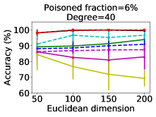
Results. First, we study the influence from the intrinsic dimensionality. We set the Euclidean dimensionality to be and vary the polynomial function’s degree from to in Figure 2a and 2d. Then, we fix the degree to be and vary the Euclidean dimensionality in Figure 2b and 2e. We can observe that the accuracies of most methods dramatically decrease when the degree (intrinsic dimension) increases, and the influence from the intrinsic dimension is more significant than that from the Euclidean dimension, which is in agreement with our theoretical analysis.
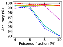
We also study their classification performances under different poisoned fraction in Figure 2c and 2f. We can see that all the defenses yield lower accuracies when the poisoned fraction increases, while the performance of DBSCAN keeps much more stable compared with other defenses. Moreover, we calculate the widely used scores from the sanitization defenses for identifying the outliers. Loss and k-NN both yield very low scores (); that means they are not quite capable to identify the real poisoning data items. The scores yielded by DBSCAN, L and Slab are shown in Figure 2g-2i, where DBSCAN in general outperforms the other two sanitization defenses for most cases.
We also perform the experiments on the real datasets under Min-Max attack with the poisoned fraction ranging from to . The experimental results (Figure 3) reveal the similar trends as the results for the synthetic datasets, and DBSCAN keeps considerably better performance compared with other defenses. Due to the space limit, the results under ALFA attack are shown in Appendix.
6 Discussion
In this paper, we study two different strategies for protecting SVM against poisoning attacks. We also have several open questions to study in future. For example, what about the complexities of other machine learning problems under the adversarially-resilient formulations as Definition 1? For many other adversarial machine learning problems, the study on their complexities is still in its infancy.
References
- Amsaleg et al. [2017] Laurent Amsaleg, James Bailey, Dominique Barbe, Sarah M. Erfani, Michael E. Houle, Vinh Nguyen, and Milos Radovanovic. The vulnerability of learning to adversarial perturbation increases with intrinsic dimensionality. In 2017 IEEE Workshop on Information Forensics and Security, WIFS, pages 1–6. IEEE, 2017.
- Barreno et al. [2006] Marco Barreno, Blaine Nelson, Russell Sears, Anthony D. Joseph, and J. D. Tygar. Can machine learning be secure? In Proceedings of the 2006 ACM Symposium on Information, Computer and Communications Security, ASIACCS, pages 16–25. ACM, 2006.
- Biggio and Roli [2018] Battista Biggio and Fabio Roli. Wild patterns: Ten years after the rise of adversarial machine learning. Pattern Recognition, 84:317–331, 2018.
- Biggio et al. [2012] Battista Biggio, Blaine Nelson, and Pavel Laskov. Poisoning attacks against support vector machines. In Proceedings of the 29th International Conference on Machine Learning, ICML, 2012.
- Biggio et al. [2014] Battista Biggio, Samuel Rota Bulò, Ignazio Pillai, Michele Mura, Eyasu Zemene Mequanint, Marcello Pelillo, and Fabio Roli. Poisoning complete-linkage hierarchical clustering. In Structural, Syntactic, and Statistical Pattern Recognition - Joint IAPR, 2014.
- Bshouty et al. [2009] Nader H. Bshouty, Yi Li, and Philip M. Long. Using the doubling dimension to analyze the generalization of learning algorithms. J. Comput. Syst. Sci., 75(6):323–335, 2009.
- Chandola et al. [2009] Varun Chandola, Arindam Banerjee, and Vipin Kumar. Anomaly detection: A survey. ACM Computing Surveys, 41(3):15, 2009.
- Chang and Lin [2011] Chih-Chung Chang and Chih-Jen Lin. LIBSVM: A library for support vector machines. ACM TIST, 2(3), 2011.
- Christmann and Steinwart [2004] Andreas Christmann and Ingo Steinwart. On robustness properties of convex risk minimization methods for pattern recognition. J. Mach. Learn. Res., 5:1007–1034, 2004.
- Cortes and Vapnik [1995] Corinna Cortes and Vladimir Vapnik. Support-vector networks. Machine Learning, 20:273, 1995.
- Cretu et al. [2008] Gabriela F. Cretu, Angelos Stavrou, Michael E. Locasto, Salvatore J. Stolfo, and Angelos D. Keromytis. Casting out demons: Sanitizing training data for anomaly sensors. In 2008 IEEE Symposium on Security and Privacy, pages 81–95. IEEE Computer Society, 2008.
- Crisp and Burges [1999] David J. Crisp and Christopher J. C. Burges. A geometric interpretation of v-SVM classifiers. In NIPS, pages 244–250. The MIT Press, 1999.
- Dalvi et al. [2004] Nilesh N. Dalvi, Pedro M. Domingos, Mausam, Sumit K. Sanghai, and Deepak Verma. Adversarial classification. In Proceedings of the Tenth ACM SIGKDD International Conference on Knowledge Discovery and Data Mining, pages 99–108, 2004.
- Ester et al. [1996] Martin Ester, Hans-Peter Kriegel, Jörg Sander, and Xiaowei Xu. A density-based algorithm for discovering clusters in large spatial databases with noise. In Proceedings of the ACM SIGKDD International Conference on Knowledge Discovery and Data Mining, pages 226–231, 1996.
- Feldman and Langberg [2011] Dan Feldman and Michael Langberg. A unified framework for approximating and clustering data. In Proceedings of the 43rd ACM Symposium on Theory of Computing, STOC, pages 569–578. ACM, 2011.
- Feng et al. [2014] Jiashi Feng, Huan Xu, Shie Mannor, and Shuicheng Yan. Robust logistic regression and classification. In Advances in Neural Information Processing Systems, pages 253–261, 2014.
- Gan and Tao [2015] Junhao Gan and Yufei Tao. DBSCAN revisited: mis-claim, un-fixability, and approximation. In Proceedings of the 2015 ACM SIGMOD International Conference on Management of Data, pages 519–530, 2015.
- Goodfellow et al. [2018] Ian J. Goodfellow, Patrick D. McDaniel, and Nicolas Papernot. Making machine learning robust against adversarial inputs. Commun. ACM, 61(7):56–66, 2018.
- Huang et al. [2011] Ling Huang, Anthony D Joseph, Blaine Nelson, Benjamin IP Rubinstein, and J Doug Tygar. Adversarial machine learning. In Proceedings of the 4th ACM workshop on Security and artificial intelligence, pages 43–58, 2011.
- Huang et al. [2018] Lingxiao Huang, Shaofeng Jiang, Jian Li, and Xuan Wu. Epsilon-coresets for clustering (with outliers) in doubling metrics. In 59th IEEE Annual Symposium on Foundations of Computer Science, FOCS, pages 814–825, 2018.
- Jagielski et al. [2018] Matthew Jagielski, Alina Oprea, Battista Biggio, Chang Liu, Cristina Nita-Rotaru, and Bo Li. Manipulating machine learning: Poisoning attacks and countermeasures for regression learning. In Symposium on Security and Privacy, SP, pages 19–35, 2018.
- Kanamori et al. [2017] Takafumi Kanamori, Shuhei Fujiwara, and Akiko Takeda. Breakdown point of robust support vector machines. Entropy, 19(2):83, 2017.
- Khoury and Hadfield-Menell [2019] Marc Khoury and Dylan Hadfield-Menell. Adversarial training with voronoi constraints. CoRR, abs/1905.01019, 2019.
- Koh et al. [2018] Pang Wei Koh, Jacob Steinhardt, and Percy Liang. Stronger data poisoning attacks break data sanitization defenses. CoRR, abs/1811.00741, 2018.
- Laishram and Phoha [2016] Ricky Laishram and Vir Virander Phoha. Curie: A method for protecting SVM classifier from poisoning attack. CoRR, abs/1606.01584, 2016.
- Li et al. [2001] Yi Li, Philip M. Long, and Aravind Srinivasan. Improved bounds on the sample complexity of learning. J. Comput. Syst. Sci., 62(3):516–527, 2001.
- Ma et al. [2018] Xingjun Ma, Bo Li, Yisen Wang, Sarah M. Erfani, Sudanthi N. R. Wijewickrema, Grant Schoenebeck, Dawn Song, Michael E. Houle, and James Bailey. Characterizing adversarial subspaces using local intrinsic dimensionality. In 6th International Conference on Learning Representations, ICLR. OpenReview.net, 2018.
- Megiddo [1990] Nimrod Megiddo. On the complexity of some geometric problems in unbounded dimension. J. Symb. Comput., 10(3/4):327–334, 1990.
- Mei and Zhu [2015] Shike Mei and Xiaojin Zhu. Using machine teaching to identify optimal training-set attacks on machine learners. In AAAI, pages 2871–2877. AAAI Press, 2015.
- Mount et al. [2014] David M. Mount, Nathan S. Netanyahu, Christine D. Piatko, Ruth Silverman, and Angela Y. Wu. On the least trimmed squares estimator. Algorithmica, 69(1):148–183, 2014.
- Natarajan et al. [2013] Nagarajan Natarajan, Inderjit S. Dhillon, Pradeep Ravikumar, and Ambuj Tewari. Learning with noisy labels. In Advances in Neural Information Processing Systems, pages 1196–1204, 2013.
- Paudice et al. [2018a] Andrea Paudice, Luis Muñoz-González, András György, and Emil C. Lupu. Detection of adversarial training examples in poisoning attacks through anomaly detection. CoRR, abs/1802.03041, 2018a.
- Paudice et al. [2018b] Andrea Paudice, Luis Muñoz-González, and Emil C. Lupu. Label sanitization against label flipping poisoning attacks. In ECML PKDD 2018 Workshops, pages 5–15, 2018b.
- Rousseeuw and Leroy [1987] Peter J. Rousseeuw and Annick Leroy. Robust Regression and Outlier Detection. Wiley, 1987.
- Rubinstein et al. [2009] Benjamin I. P. Rubinstein, Blaine Nelson, Ling Huang, Anthony D. Joseph, Shing-hon Lau, Satish Rao, Nina Taft, and J. D. Tygar. ANTIDOTE: understanding and defending against poisoning of anomaly detectors. In Proceedings of the 9th ACM SIGCOMM Internet Measurement Conference, IMC, pages 1–14. ACM, 2009.
- Scholkopf et al. [2000] B. Scholkopf, A. J. Smola, K. R. Muller, and P. L. Bartlett. New support vector algorithms. Neural Computation, 12:1207–1245, 2000.
- Schubert et al. [2017] Erich Schubert, Jörg Sander, Martin Ester, Hans Peter Kriegel, and Xiaowei Xu. DBSCAN revisited, revisited: why and how you should (still) use dbscan. ACM Transactions on Database Systems (TODS), 42(3):19, 2017.
- Simonov et al. [2019] Kirill Simonov, Fedor V. Fomin, Petr A. Golovach, and Fahad Panolan. Refined complexity of PCA with outliers. In Proceedings of the 36th International Conference on Machine Learning, ICML, pages 5818–5826, 2019.
- Steinhardt et al. [2017] Jacob Steinhardt, Pang Wei Koh, and Percy Liang. Certified defenses for data poisoning attacks. In Neural Information Processing System, pages 3517–3529, 2017.
- Suzumura et al. [2014] Shinya Suzumura, Kohei Ogawa, Masashi Sugiyama, and Ichiro Takeuchi. Outlier path: A homotopy algorithm for robust svm. In Proceedings of the 31st International Conference on Machine Learning (ICML), pages 1098–1106, 2014.
- Szegedy et al. [2014] Christian Szegedy, Wojciech Zaremba, Ilya Sutskever, Joan Bruna, Dumitru Erhan, Ian J. Goodfellow, and Rob Fergus. Intriguing properties of neural networks. In ICLR, 2014.
- Tax and Duin [1999] David M. J. Tax and Robert P. W. Duin. Support vector domain description. Pattern Recognit. Lett., 20(11-13):1191–1199, 1999.
- Tsang et al. [2005] Ivor W. Tsang, James T. Kwok, and Pak-Ming Cheung. Core vector machines: Fast SVM training on very large data sets. Journal of Machine Learning Research, 6:363–392, 2005.
- Weerasinghe et al. [2019] Sandamal Weerasinghe, Sarah M. Erfani, Tansu Alpcan, and Christopher Leckie. Support vector machines resilient against training data integrity attacks. Pattern Recognit., 96, 2019.
- Xiao et al. [2012] Han Xiao, Huang Xiao, and Claudia Eckert. Adversarial label flips attack on support vector machines. In 20th European Conference on Artificial Intelligence. Including Prestigious Applications of Artificial Intelligence, volume 242, pages 870–875. IOS Press, 2012.
- Xiao et al. [2015] Huang Xiao, Battista Biggio, Blaine Nelson, Han Xiao, Claudia Eckert, and Fabio Roli. Support vector machines under adversarial label contamination. Neurocomputing, 160:53–62, 2015.
- Xu et al. [2017] Guibiao Xu, Zheng Cao, Bao-Gang Hu, and José C. Príncipe. Robust support vector machines based on the rescaled hinge loss function. Pattern Recognit., 63:139–148, 2017.
- Xu et al. [2009] Huan Xu, Constantine Caramanis, and Shie Mannor. Robustness and regularization of support vector machines. J. Mach. Learn. Res., 10:1485–1510, 2009.
- Xu et al. [2006] Linli Xu, Koby Crammer, and Dale Schuurmans. Robust support vector machine training via convex outlier ablation. In AAAI, pages 536–542. AAAI Press, 2006.


| ALFA | Min-Max | |||||||
|---|---|---|---|---|---|---|---|---|
| DBSCAN | ||||||||
| Slab | ||||||||
| L | ||||||||
| Loss | ||||||||
| Knn | ||||||||
| ALFA | Min-Max | |||||||
|---|---|---|---|---|---|---|---|---|
| DBSCAN | ||||||||
| Slab | ||||||||
| L | ||||||||
| Loss | ||||||||
| Knn | ||||||||
| ALFA | Min-Max | |||||||
|---|---|---|---|---|---|---|---|---|
| DBSCAN | ||||||||
| Slab | ||||||||
| L | ||||||||
| Loss | ||||||||
| Knn | ||||||||