©2021 IEEE. Personal use of this material is permitted. Permission from IEEE must be obtained for all other uses, in any current or future media, including reprinting/republishing this material for advertising or promotional purposes, creating new collective works, for resale or redistribution to servers or lists, or reuse of any copyrighted component of this work in other works.
Accepted to be published in the Proceedings of the 2021 IEEE/RSJ International Conference on Intelligent Robots and Systems (IROS 2021).
DeepRelativeFusion: Dense Monocular SLAM using Single-Image Relative Depth Prediction
Abstract
Traditional monocular visual simultaneous localization and mapping (SLAM) algorithms have been extensively studied and proven to reliably recover a sparse structure and camera motion. Nevertheless, the sparse structure is still insufficient for scene interaction, e.g., visual navigation and augmented reality applications. To densify the scene reconstruction, the use of single-image absolute depth prediction from convolutional neural networks (CNNs) for filling in the missing structure has been proposed. However, the prediction accuracy tends to not generalize well on scenes that are different from the training datasets.
In this paper, we propose a dense monocular SLAM system, named DeepRelativeFusion, that is capable to recover a globally consistent 3D structure. To this end, we use a visual SLAM algorithm to reliably recover the camera poses and semi-dense depth maps of the keyframes, and then use relative depth prediction to densify the semi-dense depth maps and refine the keyframe pose-graph. To improve the semi-dense depth maps, we propose an adaptive filtering scheme, which is a structure-preserving weighted average smoothing filter that takes into account the pixel intensity and depth of the neighbouring pixels, yielding substantial reconstruction accuracy gain in densification. To perform densification, we introduce two incremental improvements upon the energy minimization framework proposed by DeepFusion: (1) an improved cost function, and (2) the use of single-image relative depth prediction. After densification, we update the keyframes with two-view consistent optimized semi-dense and dense depth maps to improve pose-graph optimization, providing a feedback loop to refine the keyframe poses for accurate scene reconstruction. Our system outperforms the state-of-the-art dense SLAM systems quantitatively in dense reconstruction accuracy by a large margin.
For more information, see the demo video and supplementary material.
I INTRODUCTION
Recovering dense structure from images can lead to many applications, ranging from augmented reality to self-driving. Visual SLAM uses only cameras to recover structure and motion, which provides cheaper solutions to the SLAM problems in comparison to light detection and ranging (LiDAR). Traditional monocular visual SLAM algorithms have shown promising sparse [1, 2, 3, 4] and semi-dense [5] reconstruction accuracy by reliably matching the texture-rich image regions such as corners and edges. While the sparse structure suffices for localizing the camera, having a dense structure could enable better interaction between a moving robot and the environment, e.g., obstacle avoidance and path planning.
Thanks to the ubiquity of graphics processing units (GPUs), computation of a dense structure from an image sequence in real-time has become possible by aggregating the photometric information in bundles of frames [6]. In general, the photometric information aggregation seeks to optimize the map by reducing the photometric re-projection errors between bundles of frames, which is a necessary but not sufficient condition to obtain a globally optimized solution. One inherent limitation is the minimization of photometric re-projection errors in textureless image regions in a bundle of frames as no distinct local minima can be found [6]. Nevertheless, one common practice in recovering depth information in texture-poor regions is to enforce a smoothness constraint [7, 8], i.e., the adjacent depth values in the texture-poor image regions change gradually.
Alternatively, the use of constraints from CNN depth [11, 12, 13] and surface normals [14, 15] predictions has been proposed to recover the 3D structure in texture-poor image regions. Both depth and surface normals provide 3D geometry information, the difference being that surface normals contain local surface orientation (i.e., the relative locations between local space points) while a depth value contains the absolute location of a space point. Therefore, the incorporation of learned 3D geometry into traditional SLAM algorithms have been proposed to solve the monocular dense reconstruction problem.
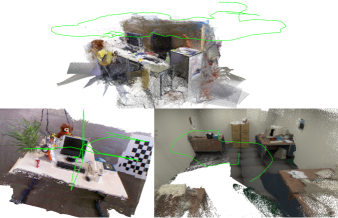
In this paper, we present a dense SLAM system that augments a monocular SLAM algorithm [5] with a dense mapping optimization framework. The optimization framework exploits the accurate depth and depth gradient information from single-image relative depth prediction as priors to densify the semi-dense structure provided by the SLAM algorithm. Next, we use the densified structure to refine the keyframe poses, while the optimized poses are combined with the densified structure to produce a globally consistent dense structure (see Figure 1). The experimental results show that our system achieves state-of-the-art dense reconstruction accuracy. Our main contributions can be summarized as follows:
-
•
To the best of our knowledge, we are the first to propose the use of single-image relative depth prediction, as opposed to absolute depth prediction, to solve the dense monocular SLAM problem.
-
•
We show, quantitatively and qualitatively, that relative depth maps result in the state-of-the-art reconstruction accuracy.
-
•
We introduce a structure-preserving and noise-reducing adaptive filter that improves the accuracy of the semi-dense structure by the monocular SLAM algorithm.
-
•
We present a method that makes use of a dense and semi-dense structure to refine the estimated camera motion, to improve its pose estimation.
II RELATED WORK
Traditional monocular SLAM algorithms are capable of producing sparse, semi-dense, and dense structures. Conceptually, sparse refers to the sparsity of the structure as well as the independence of each space point from one another during the structure and motion optimization. During the optimization, each image point (usually a corner) is being matched across frames and mapped, and collectively, the whole structure and camera motion are being optimized in the form photometric [2] or geometric [3, 1] re-projection error minimization. On the other hand, instead of processing the sparse points independently, semi-dense and dense methods employ the notion of the neighbourhood connectedness of the points. Dense methods regularize the neighbouring depth pixels using image gradient [6, 7, 8], typically formulated as a smoothness term in an energy minimization framework; whereas the semi-dense method, LSD-SLAM [5], estimates the depth values of the high gradient image regions, thus semi-dense, and regularizes the semi-dense depth map by computing each depth value the weighted average of the neighbouring depth values with the estimated variances as their weight. In this work, we use LSD-SLAM to reliably recover a semi-dense structure. Next, we filter the semi-dense structure using contextual information of the local photometric and depth information, which is inspired by the edge-preserving bilateral filtering from Tomasi and Manduchi [16]. Then, we perform densification through regularization of the structure using the filtered semi-dense structure, and depth and depth gradient information from single-image depth prediction.
There are two types of single-image depth predictions: absolute depth prediction and relative depth prediction. Absolute depth prediction problem is to train a CNN to predict the metric depth maps from single images [17, 18, 19, 20]. Because of the CNN prediction range, the CNN training is commonly limited to one scene type, e.g., indoor or outdoor dataset. On the other hand, relative depth prediction is concerned with the estimation of the distance of one space point with respect to the others, i.e., their order in depth, rather than the absolute depth. Early work on relative depth prediction learns from ordinal depth annotations (closer/farther relationship between two points), which contain fairly accurate sparse depth relationships covering a wide range of scene types (e.g., mixing indoor and outdoor scenes in a combined training dataset) [21, 22]. The training results demonstrate accurate ordinal depth prediction quantitatively on different datasets and qualitatively on unconstrained photos taken from the internet, albeit the absence of absolute depth values. To train on larger and diverse datasets, Lasinger et al. propose to train a relative depth prediction CNN, named MiDaS [23], using a scale- and shift-invariant loss, which handles unknown depth scale and global shift factors in different datasets. By eliminating the absolute scale and shift, the MiDaS’s relative depth prediction is essentially constrained to disparity space, and is akin to having surface normals prediction [24] for regularization of neighbouring space points [14, 15], and therefore is particularly suitable for our semi-dense structure densification framework.
Fusions of single-image depth prediction to visual SLAM algorithms have been proposed to solve dense reconstruction problems. One approach to performing depth fusion from multiple viewpoints is through the accumulation of probabilistic distribution of depth observations from the single-image depth prediction [11, 25]. Recently, Czarnowski et al. propose a factor-graph optimization framework named DeepFactors [13], which jointly optimizes the camera motion and the code-based depth maps. Each depth map is parameterized in an -dimensional code to avoid costly per-pixel depth map optimization. Another dense SLAM system proposed by Laidlow et al., named DeepFusion [12], uses the depth and depth gradient predictions from a CNN to constrain the optimized depth maps. Our proposed system is similar to DeepFusion, except for three key differences: (1) we use depth and depth gradient from relative depth prediction as priors in depth map optimization, (2) through extensive experimentation, we have a better cost function for performing densification, and (3) we use the densified depth maps to refine the camera pose.
III METHOD
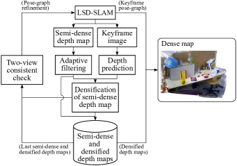
Our proposed dense SLAM system is shown in Figure 2. The system pipeline contains an optimization framework, which uses the predicted depth maps of the keyframe images (see Section III-B) and the filtered semi-dense depth maps (see Section III-C) to perform densification (see Section III-D). The optimized depth maps, in turn, are being used to optimize the keyframe pose-graph maintained by LSD-SLAM (see Section III-E). To reconstruct the scene, we back-project the densified depth maps from their respective poses obtained from the optimized keyframe pose-graph.
III-A Notation
In LSD-SLAM, the trajectory of the camera poses and the 3D location of the map points are stored in a list of keyframes. Each keyframe contains an image , a semi-dense inverse depth map , a semi-dense inverse depth variance map , and a camera pose . Note that is a subset of pixels extracted from the texture-rich image regions for the structure and camera motion estimation, and a Sim(3) camera pose is defined by:
| (1) |
where is the rotation matrix, the translation vector and the scaling factor.
III-B Depth prediction
For every new keyframe , we obtain a relative inverse depth map, hereinafter referred to as relative depth map, from MiDaS [23] for the densification of the semi-dense depth map. Because the depth prediction is a relative depth map, the predicted depth map needs to be scale- and shift-corrected before it can be used in the densification step. The scale- and shift-correction can be performed as follows:
| (2) |
where and are the scale and shift parameters, respectively. Let and , and the parameters and can be solved in closed-form as follows [23]:
| (3) |
where and are the inverse depth values of the semi-dense depth map and relative depth map, respectively.
III-C Semi-dense structure adaptive filtering
Our adaptive filtering is built upon bilateral filtering [16]. A bilateral filter is designed to combine the local pixel values according to the geometric closeness and the photometric similarity between the centre pixel and a nearby pixel within a window of an image , which is defined by:
| (4) |
with
| (5) |
In the context of semi-dense depth map filtering, we introduce two additional weighting schemes, namely, CNN depth consistency and depth uncertainty , to remove the semi-dense depth pixels that have large local variance compared to their corresponding CNN depth as well as large depth uncertainty:
| (6) |
where the squared ratio difference in computes the scale-invariant error [27], and in detects spurious depth pixels. , , and are the smoothing parameters in their respective spatial kernels. Therefore, a filtered semi-dense depth map can be computed as follows:
| (7) | ||||
with
| (8) |
and, with the updated , we re-estimate its semi-dense depth variance map by taking the average of squared deviations within the local window for all the semi-dense depth pixels:
| (9) | ||||
where is the total number of pixels within the window, the number of pixels containing depth values, and the weight computed at a nearby pixel. To remove the noisy depth pixels, we only include filtered depth whose variance is lower than a threshold . To ensure similar weighting effect of the semi-dense depth maps in densification, we rescale the semi-dense depth variance :
| (10) |
where is the mean operator.
III-D Densification of the semi-dense structure
Consider the densification of of using as initial values: the estimated inverse dense depth map can be obtained through the minimization of the cost function given by:
| (11) |
The first term, CNN depth gradient regularization , enforces depth gradient consistency between and :
| (12) |
with
| (13) |
where is the cardinality of , and the gradient operator. This error term is similar to the scale-invariant mean squared error in log space used in [27]. The denominator in Equation \tagform@12 simulates the variance of the depth prediction, which provides stronger depth gradient regularization to closer objects than farther objects.
III-E Pose-graph refinement
To incorporate the optimized semi-dense and dense structure into improving the keyframe poses while at the same time minimizing the influence of erroneous regions within the structure, we introduce a two-view consistency check step to filter the inconsistent depth regions between the current keyframe and the last keyframe . To check for structural consistency, we project the last keyframe semi-dense and densified depth maps to the current keyframe’s viewpoint:
| (15) |
where is a placeholder for and and the warped and in ’s viewpoint. To retain the semi-dense structure in LSD-SLAM, the semi-dense depth regions in has been excluded when warping . is in homogeneous coordinates, and is the camera intrinsics. The two-view consistent depth map is given by:
| (16) |
Next, we propagate the pose uncertainty estimated by LSD-SLAM to approximate the uncertainty associated with :
| (17) |
where is the Jacobian matrix containing the first-order partial derivatives of the camera projection function with respect to the camera pose [29]. As the two-view consistent depth contains a mixture of semi-dense depth regions and densified depth regions, the corresponding variance is sampled from in the semi-dense depth regions and from otherwise. After obtaining two-view consistent depth and depth variance maps, we update the Sim(3) constraints in the pose-graph to refine the keyframe poses.
IV IMPLEMENTATION
Our dense SLAM pipeline is implemented using PyTorch [30] Multiprocessing111https://pytorch.org/docs/stable/multiprocessing.html, which allows for parallel processing of the depth prediction module and the dense mapping module. To speed up computation, we use Boost.Python222https://github.com/boostorg/python to process loops and deserialize ROS messages333http://wiki.ros.org/msg.
To perform semi-dense structure adaptive filtering, we use a local window size of and the following parameter values: and .
For the energy minimization, we use PyTorch Autograd [31] with Adam optimizer [32], where the learning rate is set to 0.05. To compute the cost function, we set the weighting of the error terms to , and the generalized Charbonnier function [28] parameters are set to and . The number of optimization iterations is set to 30. The images have been resized to before the depth prediction and densification steps.
For obtaining two-view consistent depth regions, we use an error threshold of .
In LSD-SLAM, we use the original parameter settings with the exception of setting the minUseGrad parameter to 1 for the following sequences: ICL/office0, ICL/living1, and TUM/seq2 (see Table I) and both KFUsageWeight and KFDistWeight parameters to 7.5. The frame-rate of all image sequences is set to 5 to allow for better synchronization between the camera tracking and the visualization of the dense map; the increase in frame-rate theoretically should not affect the dense reconstruction performance except for the delayed visualization of the dense map, thanks to the Multiprocessing implementation.
| Percentage of correct depth (%) | ||||||
| Sequence | CNN-SLAM | DeepFactors* | DeepFusion | DeepFusion†(MiDaS)* | Ours (VNLNet)* | Ours (MiDaS)* |
| ICL/office0 | 19.410 | 30.17 | 21.090 | 15.934 | 17.395 | 17.132 |
| ICL/office1 | 29.150 | 20.16 | 37.420 | 57.097 | 60.909 | 58.583 |
| ICL/office2 | 37.226 | - | 30.180 | 72.602 | 68.914 | 72.527 |
| ICL/living0 | 12.840 | 20.44 | 24.223 | 65.395 | 60.210 | 65.710 |
| ICL/living1 | 13.038 | 20.86 | 14.001 | 75.631 | 69.980 | 75.694 |
| ICL/living2 | 26.560 | - | 25.235 | 79.994 | 78.887 | 80.172 |
| TUM/seq1 | 12.477 | 29.33 | 8.069 | 69.990 | 64.862 | 66.892 |
| TUM/seq2 | 24.077 | 16.92 | 14.774 | 52.132 | 43.607 | 59.744 |
| TUM/seq3 | 27.396 | 51.85 | 27.200 | 76.433 | 75.680 | 76.395 |
| Average | 22.464 | 27.10 | 22.466 | 62.801 | 60.049 | 63.650 |
-
•
*After aligned with ground truth scale
-
•
†Our implementation of DeepFusion
V EVALUATION
In this section, we present experimental results that validate the effectiveness of our proposed method, namely (1) the adaptive filtering to improve the semi-dense depth maps for more accurate densification, (2) the cost function in our optimization framework, (3) the use of relative depth prediction for providing depth and depth gradient priors, and (4) the use of optimized depth maps to improve the keyframe poses.
V-A Reconstruction accuracy
To evaluate our system, we use ICL-NUIM [10] and TUM RGB-D [9] datasets, which contain ground truth depth maps and trajectories to measure the reconstruction accuracy. We use the reconstruction accuracy metric proposed in [11], which is defined as the percentage of the depth values with relative errors of less than . Also, we use absolute trajectory error (ATE) to measure the error of the camera trajectories. Since our system does not produce absolute scale scene reconstruction, and therefore each depth map needs to be scaled using the optimal trajectory scale (calculated with the TUM benchmark script444https://vision.in.tum.de/data/datasets/rgbd-dataset/tools) and its corresponding Sim(3) scale for depth correctness evaluation.
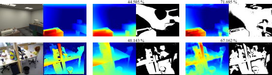
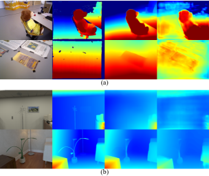
We compare our reconstruction accuracy against the state-of-the-art dense SLAM systems, namely CNN-SLAM [11], DeepFusion [12], and DeepFactors [13]. Table I shows a comparison of the reconstruction accuracy: the first three columns show the reconstruction accuracy of the state-of-the-art systems and the last two columns show a comparison between using VNLNet (an absolute depth prediction CNN) and MiDaS (a relative depth prediction CNN) in our optimization framework (see Section V-D). Owing to the similarity of the optimization frameworks between our system and DeepFusion, we also include the results for running dense reconstruction with an additional CNN depth consistency error term in the cost function (labelled ”” in Table I)555DeepFusion is not open source, and therefore the results are based on the implementation of our optimization framework (see Section IV). Our implementation of CNN depth consistency term is similar to that of DeepFusion except we use CNN depth for providing depth uncertainty (similar to Equation \tagform@12).. Note that the reconstruction accuracy of our method is taken with an average of 5 runs. Our method outperforms the competitors except for the ICL/office0 sequence, as LSD-SLAM is unable to generate a good semi-dense structure under rotational motion, hence the degraded reconstruction performance in the densification of the semi-dense structure. The reconstruction results demonstrate the superiority of our system by comparing the last column with all other columns in Table I. Figure 3 shows the use of our optimization framework to obtain more accurate densified depth maps from less accurate predicted relative depth maps.
| Percentage of correct depth (%) | |||
| Energy term | ICL/living2 | ICL/office2 | TUM/seq1 |
| 1 | 62.620 | 57.563 | 55.031 |
| 1(c) | 65.611 | 57.644 | 55.042 |
| 1(f)(c) | 71.265 | 61.445 | 60.143 |
| 1(c)+2∘ | 69.967 | 69.905 | 64.650 |
| 1(f)(c)+2∘ | 79.788 | 71.778 | 67.319 |
| 1(c)+2+3⋄ | 70.167 | 69.863 | 64.730 |
| 1(f)(c)+2+3⋄ | 79.742 | 71.692 | 67.323 |
| 1. SLAM depth consistency | |||
| 2. CNN depth gradient consistency | |||
| 3. CNN depth consistency | |||
| (c). Generalized Charbonnier function† | |||
| (f). Adaptive semi-dense depth filtering† | |||
V-B Adaptive filtering results
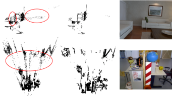
We notice that the semi-dense structure from LSD-SLAM contains spurious map points, which may worsen the dense reconstruction performance. Figure 4 shows a qualitative comparison between the semi-dense depth maps by LSD-SLAM and the filtered depth maps, demonstrating the effectiveness of the adaptive filter in eliminating noisy depth pixels while preserving the structure of the scene. Quantitatively, the second row and the third row of Table II (labelled ”f”) shows about improvement on using adaptive filtering in dense reconstruction (see also the last four rows).
V-C Cost function analysis
Table II shows the reconstruction results using different combinations of error terms in the cost function. To ensure consistent measurement of the reconstruction accuracy using different cost functions, the keyframes—i.e., the semi-dense depth and depth variance maps, and the camera poses—are pre-saved so that the densification process is not influenced by the inconsistency between runs from LSD-SLAM. Consistent with the finding in DeepFusion, incorporation of CNN depth gradient consistency and CNN depth consistency improves the reconstruction accuracy dramatically, although our CNN does not explicitly predict depth gradient and depth gradient variance maps (see the second and last row). However, removing the CNN depth consistency term (the the third and fourth last row), in our case, leads to better reconstruction accuracy (see also the third last and last column of Table I); the added generalized Charbonnier function (the second row, and labelled ”c”) also increases the accuracy.
| Percentage of correct depth (%) | |||
| Sequence | Laina (abs) | VNLNet (abs)* | MiDaS (rel)* |
| ICL/office0 | 17.194 | 11.791 | 13.059 |
| ICL/office1 | 20.838 | 45.866 | 42.980 |
| ICL/office2 | 30.639 | 55.180 | 55.136 |
| ICL/living0 | 15.008 | 40.294 | 54.287 |
| ICL/living1 | 11.449 | 55.806 | 72.139 |
| ICL/living2 | 33.010 | 59.367 | 67.130 |
| TUM/seq1 | 12.982 | 47.552 | 54.860 |
| TUM/seq2 | 15.412 | 33.143 | 55.136 |
| TUM/seq3 | 9.450 | 52.144 | 57.255 |
| Average | 18.452 | 44.571 | 52.442 |
-
•
*After scale- and shift-correction
V-D Relative depth prediction vs. absolute depth prediction
To illustrate the advantage of using relative depth prediction CNNs (e.g., MiDaS), we perform the same densification step with an absolute depth prediction CNN, VNLNet666One important consideration in selecting a competing absolute depth prediction CNN is the runtime memory requirements. VNLNet is considered state-of-the-art at the time of experimental setup with a reasonable memory footprint. [20], and then compare the reconstruction accuracy between them. To promote a fair comparison, neither MiDaS nor VNLNet has been trained on the TUM RGB-D and ICL-NUIM datasets. In Table I, we show that, in general, using scale- and shift-corrected relative depth prediction (labelled ”MiDaS”) instead of absolute depth prediction (other columns) has superior dense reconstruction performance, as a result of more accurate depth prediction from MiDaS than depth prediction from VNLNet (last and second last column of Table III); Laina (second column of Table III), another absolute depth prediction CNN being used in CNN-SLAM, is significantly less accurate than MiDaS, which indicates that the outperformance of our system may just simply be due to the fact that MiDaS provides more accurate depth prediction for densification. Not only are the scale- and shift-corrected relative depth maps from MiDaS metrically more accurate than the absolute depth maps from VNLNet, but the relative depth maps also appear to be smoother (see Figure 5).
V-E Keyframe trajectory accuracy
Table IV shows the camera tracking accuracy between our method and CNN-SLAM777Only CNN-SLAM has the ATEs on the evaluation datasets.. From the first two columns, we can see that our camera tracking performance, even without the pose-graph refinement, reduces the ATE of CNN-SLAM by almost . Since both of the systems are built upon LSD-SLAM, the performance difference could be due to our configuration settings in LSD-SLAM (see Section IV). To evaluate the effectiveness of pose-graph refinement, the last column shows a baseline performance of refining the pose-graph using ground truth depth. In general, pose-graph refinement reduces the ATE significantly to the extent that, in certain sequences, it is similar to that obtained by pose-graph refinement using the ground truth depth.
| Absolute trajectory error (m) | ||||
| Sequence | CNN-SLAM | Ours⋄ | Ours∘ | Ours* |
| ICL/office0 | 0.266 | 0.352 | 0.295 | 0.260 |
| ICL/office1 | 0.157 | 0.057 | 0.046 | 0.045 |
| ICL/office2 | 0.213 | 0.159 | 0.061 | 0.045 |
| ICL/living0 | 0.196 | 0.057 | 0.039 | 0.036 |
| ICL/living1 | 0.059 | 0.017 | 0.018 | 0.017 |
| ICL/living2 | 0.323 | 0.062 | 0.059 | 0.056 |
| TUM/seq1 | 0.542 | 0.103 | 0.075 | - |
| TUM/seq2 | 0.243 | 0.261 | 0.245 | - |
| TUM/seq3 | 0.214 | 0.108 | 0.111 | - |
| Average | 0.246 | 0.131 | 0.106 | - |
-
•
-Not evaluated as not all the images have a corresponding depth map
V-F Timing evaluation
On average, the CNN depth prediction and optimization require 0.15 s and 0.2 s, respectively, to complete. The measurements are taken on a laptop computer equipped with an Intel 7820HK CPU and an Nvidia GTX 1070 GPU.
VI DISCUSSION
This study illustrates the potential capability of combining a relative depth prediction CNN with a visual SLAM algorithm in solving the dense monocular reconstruction problem. One of the major bottlenecks of the state-of-the-art dense SLAM systems is the accurate depth prediction requirement in the testing scene. While the use of absolute depth prediction may help produce absolute scale reconstruction, it mostly makes sense in the context narrow application domain, such as dense scene reconstruction for self-driving cars. With the proposed use of relative depth prediction, we improve the versatility of our system by forgoing absolute scale reconstruction, which can be easily recovered using fiducial markers or objects with known scales. With accurate relative depth prediction as well as continuous expansion in single-image relative depth CNN training datasets, we are getting closer to solving dense monocular SLAM in the wild—dense scene reconstruction on arbitrary image sequences.
VII CONCLUSION
In this paper, we have presented a real-time dense SLAM system, named DeepRelativeFusion, that exploits the depth and depth gradient priors provided by a relative depth prediction CNN. Our system densifies a semi-dense structure provided by LSD-SLAM through a GPU-based energy minimization framework. Through ablation study, we have validated the effectiveness of the cost function used for densification, which examines the contribution of the error terms to the dense reconstruction accuracy. Our proposed adaptive filtering has been shown to remove spurious depth pixels in the semi-dense depth maps while preserving the structure, and this in turn improves the reconstruction accuracy. To further improve the dense reconstruction accuracy, we have presented a technique that uses two-view consistent optimized depth maps to refine the keyframe poses. With the accurate relative depth prediction on diverse scene types, the use of a relative depth prediction CNN is a promising step towards dense scene reconstruction in unconstrained environments.
However, the densified structure does not benefit from the refined camera motion. Motivated by the major progress in integrating depth, pose and uncertainty predictions into front-end camera tracking and back-end bundle adjustment to continuously optimize sparse structure and camera motion [37, 38, 39], in the future, we will look into effective ways to continuously refine dense structure and camera motion.
References
- [1] C. Forster, M. Pizzoli, and D. Scaramuzza, “SVO: Fast Semi-Direct Monocular Visual Odometry,” in Proc. IEEE International Conference on Robotics and Automation (ICRA’14), pp. 15–22, IEEE, May 2014.
- [2] J. Engel, V. Koltun, and D. Cremers, “Direct Sparse Odometry,” IEEE Trans. Pattern Anal. Mach. Intell., vol. 40, no. 3, pp. 611–625, 2018.
- [3] R. Mur-Artal, J. M. M. Montiel, and J. D. Tardos, “ORB-SLAM: A Versatile and Accurate Monocular SLAM System,” IEEE Trans. Robot., vol. 31, no. 5, pp. 1147–1163, 2015.
- [4] Q. Fu, H. Yu, X. Wang, Z. Yang, H. Zhang, and A. Mian, “FastORB-SLAM: Fast ORB-SLAM method with Coarse-to-Fine Descriptor Independent Keyframe Matching,” in arXiv:2008.09870, 2020.
- [5] J. Engel, T. Schps, and D. Cremers, “LSD-SLAM: Large-scale Direct Monocular SLAM,” in Proc. European Conference on Computer Vision (ECCV’14), (Zurich, Switzerland), pp. 834–849, Springer, Sept. 2014.
- [6] R. A. Newcombe, S. J. Lovegrove, and A. J. Davison, “Dtam: Dense tracking and mapping in real-time,” in 2011 international conference on computer vision, pp. 2320–2327, IEEE, 2011.
- [7] R. A. Newcombe and A. J. Davison, “Live dense reconstruction with a single moving camera,” in 2010 IEEE Computer Society Conference on Computer Vision and Pattern Recognition, pp. 1498–1505, IEEE, 2010.
- [8] J. Stühmer, S. Gumhold, and D. Cremers, “Real-time dense geometry from a handheld camera,” in Joint Pattern Recognition Symposium, pp. 11–20, Springer, 2010.
- [9] J. Sturm, N. Engelhard, F. Endres, W. Burgard, and D. Cremers, “A benchmark for the evaluation of rgb-d slam systems,” in Proc. of the International Conference on Intelligent Robot Systems (IROS), Oct. 2012.
- [10] A. Handa, T. Whelan, J. McDonald, and A. Davison, “A benchmark for RGB-D visual odometry, 3D reconstruction and SLAM,” in IEEE Intl. Conf. on Robotics and Automation, ICRA, May 2014.
- [11] K. Tateno, F. Tombari, I. Laina, and N. Navab, “Cnn-slam: Real-time dense monocular slam with learned depth prediction,” in Proceedings of the IEEE Conference on Computer Vision and Pattern Recognition, pp. 6243–6252, 2017.
- [12] T. Laidlow, J. Czarnowski, and S. Leutenegger, “Deepfusion: Real-time dense 3d reconstruction for monocular slam using single-view depth and gradient predictions,” in 2019 International Conference on Robotics and Automation (ICRA), pp. 4068–4074, IEEE, 2019.
- [13] J. Czarnowski, T. Laidlow, R. Clark, and A. J. Davison, “Deepfactors: Real-time probabilistic dense monocular slam,” IEEE Robotics and Automation Letters, pp. 721–728, 2020.
- [14] J. Tang, J. Folkesson, and P. Jensfelt, “Sparse2dense: From direct sparse odometry to dense 3-d reconstruction,” IEEE Robotics and Automation Letters, vol. 4, no. 2, pp. 530–537, 2019.
- [15] C. S. Weerasekera, Y. Latif, R. Garg, and I. Reid, “Dense monocular reconstruction using surface normals,” in 2017 IEEE International Conference on Robotics and Automation (ICRA), pp. 2524–2531, IEEE, 2017.
- [16] C. Tomasi, and R. Manduchi, “Bilateral Filtering for Gray and Color Images,” in Proceedings of the IEEE International Conference on Computer Vision, pp. 839–846, 1998.
- [17] A. J. Amiri, S. Y. Loo, and H. Zhang, “Semi-supervised monocular depth estimation with left-right consistency using deep neural network,” in 2019 IEEE International Conference on Robotics and Biomimetics (ROBIO), pp. 602–607, 2019.
- [18] C. Godard, O. M. Aodha, and G. J. Brostow, “Unsupervised Monocular Depth Estimation with Left-Right Consistency,” in Proc. IEEE Conference on Computer Vision and Pattern Recognition (CVPR’17), (Honolulu, Hawaii), IEEE, July 2017.
- [19] X. Qi, R. Liao, Z. Liu, R. Urtasun, and J. Jia, “Geonet: Geometric neural network for joint depth and surface normal estimation,” in Proceedings of the IEEE Conference on Computer Vision and Pattern Recognition, pp. 283–291, 2018.
- [20] W. Yin, Y. Liu, C. Shen, and Y. Yan, “Enforcing geometric constraints of virtual normal for depth prediction,” in Proceedings of the IEEE International Conference on Computer Vision, pp. 5684–5693, 2019.
- [21] D. Zoran, P. Isola, D. Krishnan, and W. T. Freeman, “Learning ordinal relationships for mid-level vision,” in Proceedings of the IEEE International Conference on Computer Vision, pp. 388–396, 2015.
- [22] W. Chen, Z. Fu, D. Yang, and J. Deng, “Single-image depth perception in the wild,” in Advances in neural information processing systems, pp. 730–738, 2016.
- [23] R. Ranftl, K. Lasinger, D. Hafner, K. Schindler, and V. Koltun, “Towards robust monocular depth estimation: Mixing datasets for zero-shot cross-dataset transfer,” IEEE Transactions on Pattern Analysis and Machine Intelligence (TPAMI), 2020.
- [24] W. Yin, X. Wang, C. Shen, Y. Liu, Z. Tian, S. Xu, and C. Sun, “Diversedepth: Affine-invariant depth prediction using diverse data,” in arxiv: 2002.00569, 2020.
- [25] C. Liu, J. Gu, K. Kim, S. G. Narasimhan, and J. Kautz, “Neural rgb (r) d sensing: Depth and uncertainty from a video camera,” in Proceedings of the IEEE Conference on Computer Vision and Pattern Recognition, pp. 10986–10995, 2019.
- [26] J. Bian, Z. Li, N. Wang, H. Zhan, C. Shen, M.-M. Cheng, and I. Reid, “Unsupervised scale-consistent depth and ego-motion learning from monocular video,” in Advances in Neural Information Processing Systems, pp. 35–45, 2019.
- [27] D. Eigen, C. Puhrsch, and R. Fergus, “Depth map prediction from a single image using a multi-scale deep network,” in Advances in neural information processing systems, pp. 2366–2374, 2014.
- [28] J. T. Barron, “A general and adaptive robust loss function,” in Proceedings of the IEEE Conference on Computer Vision and Pattern Recognition, pp. 4331–4339, 2019.
- [29] H. Strasdat, “Local accuracy and global consistency for efficient visual SLAM, ”, PhD thesis, Department of Computing, Imperial College London, 2012.
- [30] A. Paszke, S. Gross, F. Massa, A. Lerer, J. Bradbury, G. Chanan, T. Killeen, Z. Lin, N. Gimelshein, L. Antiga, A. Desmaison, A. Kopf, E. Yang, Z. DeVito, M. Raison, A. Tejani, S. Chilamkurthy, B. Steiner, L. Fang, J. Bai, and S. Chintala, “Pytorch: An imperative style, high-performance deep learning library,” in Advances in Neural Information Processing Systems 32 (H. Wallach, H. Larochelle, A. Beygelzimer, F. d'Alché-Buc, E. Fox, and R. Garnett, eds.), pp. 8024–8035, Curran Associates, Inc., 2019.
- [31] A. Paszke, S. Gross, S. Chintala, G. Chanan, E. Yang, Z. DeVito, Z. Lin, A. Desmaison, L. Antiga, and A. Lerer, “Automatic differentiation in pytorch,” in NeurIPS Workshop, 2017.
- [32] D. P. Kingma and J. Ba, “Adam: A method for stochastic optimization,” arXiv preprint arXiv:1412.6980, 2014.
- [33] I. Laina, C. Rupprecht, V. Belagiannis, F. Tombari, and N. Navab, “Deeper depth prediction with fully convolutional residual networks,” in 2016 Fourth international conference on 3D vision (3DV), pp. 239–248, IEEE, 2016.
- [34] Z. Li and N. Snavely, “Megadepth: Learning single-view depth prediction from internet photos,” in Proceedings of the IEEE Conference on Computer Vision and Pattern Recognition, pp. 2041–2050, 2018.
- [35] W. Maddern, G. Pascoe, C. Linegar, and P. Newman, “1 year, 1000 km: The oxford robotcar dataset,” The International Journal of Robotics Research, vol. 36, no. 1, pp. 3–15, 2017.
- [36] J. Engel, V. Usenko, and D. Cremers, “A photometrically calibrated benchmark for monocular visual odometry,” in arXiv:1607.02555, July 2016.
- [37] N. Yang, L. von Stumberg, R. Wang, and D. Cremers, “D3vo: Deep depth, deep pose and deep uncertainty for monocular visual odometry,” Proceedings of the IEEE/CVF Conference on Computer Vision and Pattern Recognition, pp. 1281–1292, 2020.
- [38] S. Y. Loo, A. J. Amiri, S. Mashohor, S. H. Tang, and H. Zhang, “CNN-SVO: Improving the mapping in semi-direct visual odometry using single-image depth prediction,” in International Conference on Robotics and Automation (ICRA), pp. 5218–5223, 2019.
- [39] R. Cheng, C. Agia, D. Meger, G. Dudek, “Depth Prediction for Monocular Direct Visual Odometry,” in Conference on Computer and Robot Vision (CRV), pp. 70–77, 2020.