Deep water wave cloaking using a multi-layered buoyant plate
Abstract
Trajectory of surface gravity waves in potential flow regime is affected by the gravitational acceleration, water density, and sea bed depth. While the gravitational acceleration and water density are approximately constant, and the effect of water depth on surface gravity waves exponentially decreases as the water depth increases. In shallow water, cloaking an object from surface waves by varying the sea bed topography is possible, however, as the water depth increases, cloaking becomes a challenge since there is no physical parameter to be engineered and subsequently affect the wave propagation. In order to create an omnidirectional cylindrical cloaking device for finite-depth/deep-water waves, we propose a multi-layered elastic plate that floats on the surface around a to-be-cloaked cylinder. The buoyant elastic plate is made of axisymmetric, homogeneous, and isotropic layers which provides adjustable degrees of freedom to engineer and affect the wave propagation. We first develop a pseudo-spectral method to efficiently determine the wave solution for a multi-layered buoyant plate. Next, we optimize the physical parameters of the buoyant plate (i.e. elasticity and mass of every layer) using a real-coded evolutionary algorithm to minimize the energy of scattered-waves from the object and therefore cloak the inner cylinder from incident waves. We show that the optimized cloak reduces the energy of scattered-waves as high as 99.2% for the target wave number. We quantify the effectiveness of our cloak with different parameters of the buoyant plate and show that varying the flexural rigidity is essential to control wave propagation and the cloaking structure needs to be at least made of four layers with a radius of at least three times of the cloaked region. We quantify the wave drift force exerted on the structures and show that the buoyant plate reduces the exerted force by 99.9%. The proposed cloak, due to its structural simplicity and effectiveness in reducing the wave drift force, may have potential applications in cloaking offshore structures from deep water waves.
keywords:
cloaking, deep water waves, multi-layered buoyant plate, scattering cancellation, evolutionary optimization1 Introduction
To safely operate and maintain offshore structures in deep water, such as column-based (spar-type) wind turbines or floating platforms, over a long period of time, the reduction of the wave drift force (time-averaged second-order hydrodynamic force) is essential. Additionally, creating a calm and cloaked region on the ocean surface in presence of surface waves facilitates the installation of these offshore structures. The concept of cloaking objects from incident waves was initially developed for electromagnetic waves Pendry et al. (2006); Schurig et al. (2006). A cloak is a structure that encloses a to-be-cloaked object and results in no reflection or scattering of incident waves from the object. The downstream waves bears no information of the object’s presence and the cloaked region is secluded from incident waves. The cloaks proposed for the electromagnetic waves are based on the idea of transformation optics and exploit the form-invariance of governing equations. The material properties of the cloak are found using spatial transformations of governing equations. The obtained material properties are usually inhomogeneous and orthotropic and implementing such properties results in the desired trajectory of the incoming waves. Since the only property used in this technique is the form-invariance of the governing equations under spatial coordinate transformation, this method has been extended to other areas of physics with form-invariant governing equations, such as acoustics Cummer & Schurig (2007); Chen & Chan (2007); Huang et al. (2014); Zareei et al. (2018); Darabi et al. (2018a), elastic waves Farhat & Enoch (2009); Stenger & Wegener (2012); Darabi et al. (2018b); Zareei & Alam (2017), or seismic waves Brûlé et al. (2014). Besides transformation techniques, an alternative method to achieve cloaking is to minimize the scattering cross-section (or energy of scattered-waves) of an object Alù & Engheta (2005). This method has also been successfully applied to different types of waves such as acoustic waves Guild et al. (2011) or water waves Porter (2011); Porter & Newman (2014).
In shallow water, cloaking has been realized using the coordinate transformation technique Berraquero et al. (2013); Zareei & Alam (2015). The governing equation of shallow water gravity waves is form-invariant under the coordinate transformation. The physical parameters controlling wave propagation in shallow water are the sea bed topography and the gravitational acceleration (e.g. Berraquero et al., 2013; Zareei & Alam, 2015). Clearly varying the gravitational acceleration is unrealistic. The use of nonlinear transformation of cylindrical region can keep the gravitational acceleration a constant value, and only changes in the sea bed topography is used to achieve cloaking from shallow water waves Zareei & Alam (2015). Alternative approaches are to use an array of bottom-mounted objects for implementing a cloaking devices for shallow water surface gravity waves using the coordinate transformation technique Dupont et al. (2016); Iida & Kashiwagi (2018), or capillary-gravity waves Farhat et al. (2008).
As the water depth increases, the effect of the bottom topography exponentially decreases, and as a result engineered sea bed topography does not affect the wave propagation. In addition, the governing equation of deep water waves in potential flow regime is not form-invariant under the coordinate transformation, and therefore it is hard to apply the transformation technique to make a cloak for deep water waves. To achieve cloaking in a finite depth, a scattering cancellation is proposed Porter (2011); Porter & Newman (2014). Specifically, a sea bed topography is designed to cancel the energy of scattered-waves of a bottom-mounted cylinder Porter & Newman (2014). Multiple floating cylinders (or a ring) are used and this shows cloaking performance even for deep water waves Newman (2014). This cloaking method is validated by numerical computations using a higher-order boundary element method Iida et al. (2014) and a model experiment Iida et al. (2016). Since an asymmetrical array of the cylinder is utilized, the performance of the cloak depends on the wave direction Zhang et al. (2019). A concentric annular elastic plate is optimized to reduce the wave drift force Loukogeorgaki & Kashiwagi (2019), however, the reduction of the energy of scattered-waves is not observed since the plate’s flexural rigidity is the only controllable medium property. Besides, since the flexural waves in elastic thin plates are not form-invariant Zareei & Alam (2017), the floating elastic plate cannot be used for the transformation-based cloaking in deep water.
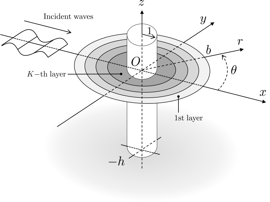
In this paper, we implement a cloak using a multi-layered elastic plate floating on the surface surrounding a to-be-cloaked cylinder in order to develop a practical and realistic offshore structure protection device from waves. The multi-layered plate is made of concentric, axisymmetric, homogeneous, and isotropic elastic layers that provide adjustable degrees of freedom in physical parameters to vary and affect the wave propagation (See Fig. 1). Medium parameters of this plate, i.e. the size, the flexural rigidity, and the mass of each layer, are optimized to cancel the energy of scattered-waves from the cylinder. First, we develop a numerical scheme for solving this problem. The scheme is based on pseudo-spectral and eigenvalue matching methods Peter et al. (2004), and this is extended to the calculation of the multi-layered plate. Next, we use an evolutionary strategy to find the optimum parameters for the floating plate. We quantify the effectiveness of our multi-layered cloak and show that the energy of scattered-waves and wave drift force acting on the structure are reduced as high as 99.2% at the target wave number. In addition, we study the effect of different parameters on the optimum solution, and show that varying the flexural rigidity is essential to cloaking performance and the cloaking structure needs to be at least be made of four layers with a radius of at least three times of the cloaked cylinder. By quantifying the wave drift force exerted on the cylinder, we show that the buoyant plate reduces the net force by 99.9% at the target wave number.
2 Formulation of the problem
2.1 Governing equation and boundary conditions
We consider a bottom-mounted cylinder with radius surrounded by a multi-layered circular elastic plate floating on the surface of the water which is expected to effectively cloak the cylinder from incident water waves (see. Fig. 1). The plate is made of horizontal layers where the mechanical properties of each layer is kept as a constant. This assumption facilitates future experimental validation of our setup. We number the layers from outer to inner and denote the outer/inner radius of the -th layer as . The outermost and innermost layers are respectively and . For simplicity of notation we will use for the outer radius unless mentioned other-wised. We consider a Cartesian coordinate system with origin at the center of the cylinder where plane coincides with the undisturbed free surface of the water and positive -axis pointing upward. Assuming a flat bottom topography at and considering that the surrounding fluid to be incompressible, inviscid, and irrotational, the linearized governing equation and boundary conditions for the fluid’s velocity potential become
| (1) | |||||
| (2) | |||||
| (3) | |||||
| (4) |
where is the gravitational acceleration, is the fluid density, is the flexural rigidity of the -th layer, is mass per unit length of the -th layer, is the gradient operator, and is the horizontal gradient operator. Flexural rigidity and mass of the cloaking plate are calculated as and where is the -th layer Young’s modulus, is the Poisson’s ratio, and and are the density and thickness of the -th layer, respectively. In the above equations, Eq. (1) is obtained by the mass conservation, Eq. (2) is a bottom kinematic boundary condition, Eq. (3) is a linearized free surface condition, and Eq. (4) is the linearized surface condition for the -th layer of the plate. Next, we non-dimensionalize the above equations, using the radius of the cylinder , incident wave amplitude , fluid density , and gravitational acceleration , where we define , , and . We further assume time-harmonic solutions, the velocity potential becomes , where is a non-dimensional frequency. Considering the above conditions, the linearized and non-dimensionalized governing equation and boundary conditions are obtained (e.g. Meylan, 2002) with dropped overbars as
| (5) | |||||
| (6) | |||||
| (7) | |||||
| (8) |
where and are non-dimensional flexural rigidity and mass of -th layer, respectively.
2.2 Spectral decomposition of velocity potential
In order to derive a spectral method solution for the above system of equations (i.e. Eqs. (5)-(8)), we use separation of variables to express the velocity potential (e.g. Newman, 1977) as,
| (9) |
Substituting Eq. (9) in Eqs. (5)-(8), the dispersion relations of water waves and elastic waves on the plate are obtained as
| (12) |
and
| (15) |
Equation (12) is the dispersion relation of water waves, where is the wave number of water waves. The wave number in Eq. (12) has infinite number of positive and real solutions, where denotes progressive waves, and , correspond to local waves (i.e. evanescent waves). Equation (15), on the other hand, is the dispersion relation of elastic waves for the -th layer of the plate, where is the wave number. Similarly, the wave number in Eq. (15) has infinite number of positive and real solutions , and additionally two complex solutions and where and the real parts are positive. Here, indicates progressive waves, are wave numbers of local waves, and and represent damped waves (e.g. Fox & Squire, 1994). Using the above dispersion relations, the solutions for are given as
| (18) |
and
| (21) |
where is the -function of the water wave region (), and is the -function of the -th layer region . Next, the solution for is given as for . Lastly, solutions with respect to are given from Bessel differential equations. Since solutions are bound by the radiation condition (i.e. only progressive waves survive at far-field), the velocity potential of water wave region is given as
| (22) |
where is the Hankel function of the first kind, is the modified Bessel function of second kind, and is an unknown coefficient of the velocity potential . The coefficient is used for normalizing and that of incident waves. Note that the velocity potential of the -th layer region is
| (23) | |||||
where is the Bessel function of first kind, is the modified Bessel function of first kind, and and are unknown coefficients. Considering incident waves coming from as , the corresponding velocity potential becomes
| (24) |
In summary, the solution to this problem, using the spectral method (e.g. Peter et al., 2004), is given as
| (27) |
The unknown coefficients , and are numerically determined to satisfy further boundary conditions. A numerical approach for solving this problem will be discussed in the numerical approach section (§3).
2.3 Energy of scattered-waves at far-field
Performance of the plate as a cloaking device is quantified by the energy of scattered-waves Iida et al. (2014). To obtain the energy of scattered-waves, we consider a control surface at the far-field that surrounds the cylinder and the plate and then calculate the flow of energy passing through this surface. The non-dimensional energy is obtained Maruo (1960); Kashiwagi et al. (2005) as
| (28) |
Since the control surface is far from the cylinder and the plate, local waves created by structures and the waves are fully attenuated, and as a result, the velocity potential at far-field becomes
| (29) |
where
| (30) |
Substituting Eq. (29) in Eq. (28), we find the energy
| (31) | |||||
where
| (32) |
Note that the orthogonal relations and Wronskian formulae are (see Kashiwagi & Yoshida, 2001)
| (33) | |||
| (37) |
where is the Kronecker delta. Using Eqs. (33) and (37), we can simplify the energy term to
| (38) |
The above equation is the energy conservation principle, and thus it must be zero (we later use this fact to check the numerical accuracy of our code). Note that since is the amplitude of scattered-waves, the second term in Eq. (38) indicates the energy transferred to scattered-waves. As a result, the energy of scattered-waves is given as
| (39) |
The energy of scattered-waves obtained here (Eq. (39)) is equal to the form of the Kochin function in Newman (2014). We define the cloaking factor by the ratio of the energy of scattered-waves of the cylinder itself and that of the cylinder with the cloak Porter & Newman (2014), i.e.
| (40) |
If then the energy scattered by the cylinder is decreased by the cloak and clearly, the perfect cloaking is achieved as .
Next, we calculate the wave drift force acting on the cylinder. The wave drift force is the time-averaged second-order hydrodynamic force calculated by the first-order velocity potential. Considering the control surface at far-field, the wave drift force can be calculated by the momentum conservation principle Maruo (1960)
| (41) |
where is the non-dimensional wave drift force, is the surface of the body, is pressure, is the -component of normal vector, and is the velocity in the direction of normal vector. Using similar analytical expansion to the energy of scattered-waves, the formula for the wave drift force is obtained Kashiwagi & Yoshida (2001)
| (42) |
Since the wave drift force is calculated by the amplitude of scattered-waves , the wave drift force acting on bodies becomes very small when there is no scattered-wave.
3 Numerical approach
The spectral solution (i.e. Eqs. (22) and (23)) to this problem (Eqs. (5)-(8)) has unknown coefficients (i.e. , and ) that can be found by satisfying the boundary conditions. At first, we approximate the solution by truncating the infinite number of modes in Eq. (27) to orders and for azimuthal and radial terms respectively. The numbers and are decided such that the solution is converged and the results do not change by increasing and any further. For each azimuthal mode, we have unknowns in the water wave region (i.e. for ), and unknowns in the plate region (i.e. and for and ). In total, the number of unknown coefficients is , and thus the same number of boundary conditions are required for solving them.
We utilize an eigenvalue matching method Peter et al. (2004) to determine the unknown coefficients. The form of the velocity potential in Eq. (27) depends on the radial direction , and matching of each quantity at the boundaries should be considered. Since these matching boundary conditions are valid throughout the depth, -function is selected as a set of basis functions. These functions are multiplied by the velocity potential, and these are integrated throughout the water depth. Resultant functions with respect to are defined as
| (43) | |||
| (44) |
Note that wave numbers in Eqs (43) and (44) must be replaced as and when . Using Eqs (43) and (44) for each boundary condition, the number of conditions becomes . Next, we need to satisfy the following boundary conditions:
-
1.
Matching conditions of the velocity potential between the free surface and the plate ( equations).
-
2.
Matching conditions of the radial derivative of the velocity potential between the free surface and the plate ( equations).
-
3.
Matching conditions of the velocity potential between adjacent layers ( equations).
-
4.
Matching conditions of the radial derivative of the velocity potential between adjacent layers ( equations).
-
5.
No flux conditions at the surface of the cylinder ( equations).
-
6.
Matching conditions of the wave elevation between adjacent layers ( equations).
-
7.
Matching conditions of the radial derivative of the wave elevation between adjacent layers ( equations).
-
8.
Matching conditions of the bending moment between adjacent layers ( equations).
-
9.
Matching conditions of the shear force between adjacent layers ( equations).
-
10.
Free-free beam conditions; zero bending moment and shear force (4 equations).
Matching the above list of boundary conditions, we obtain equations which is the same as the number of unknowns. Solving these equations, all unknown coefficients are found. Details of these boundary conditions are shown in Appendix A. For completeness, here, we calculate the bending moment and equivalent shear force on the plate using the surface elevation of the plate. These quantities for the radial direction acting on the -th layer are given as
| (45) | |||||
| (46) |
where and are written as
| (47) | |||
| (48) |
In the above equations, note that
| (49) | |||||
where
| (50) |
4 Evolutionary optimization of the plate
Our goal here is to cancel the energy of scattered-waves from the cylinder by optimizing the buoyant plate parameters. In other words, we optimize the parameters of the plate to minimize the energy of scattered-waves through a meta-heuristic approach. We use an evolutionary optimization method, specifically, the real-coded genetic algorithm (RGA) based on the unimodal normal distribution crossover and minimal generation gap Ono et al. (1999). We rewrite the problem here as
| (54) |
where optimum non-dimensional flexural rigidity and mass are sought under selected numerical conditions: the wave number , the water depth , the outermost radius of the plate , the number of layers , and the Poisson’s ratio of the plate . Note that the above minimization is done at a certain wave number of incident waves. In order to show the full frequency response of the structures, we later find the response of our structures at wave numbers different from the optimized one.
5 Results and discussions
To show the effectiveness of the proposed multi-layered cloak, numerical simulations are carried out. In order to consider the finite depth and deep water waves, we assume , where is the water depth and is the wavelength. We fix the Poisson’s ratio of the plate , and also consider the same radial width for each layer of the plate, i.e. , where is the total number of the plate’s layers. Here, we aim to cloak the cylinder at the wave number . The energy of scattered-waves of the isolated cylinder at this wave number is . To suppress this energy, we optimize plate parameters, i.e. flexural rigidity , and mass , using the evolutionary strategy at (§4). In order to optimize the plate parameters, we consider three different cases: (1) optimizing both flexural rigidity and mass for all of the layers of the plate . We call this case I; (2) optimizing the flexural rigidity for each layer of the plate (, ) while keeping the mass as a constant for all layers (i.e. ). We denote this as case II; and lastly (3) optimizing mass of the plate for each layer of the plate (, ) while keeping the flexural rigidity as a constant for all layers ( ). We call this case III.
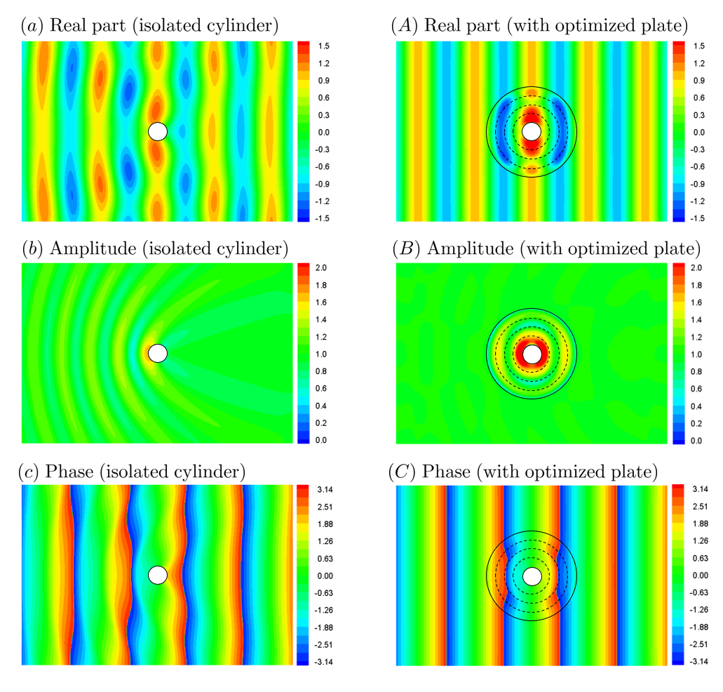
We visualize the wave field around an isolated cylinder and also a cylinder with the cloaking plate surrounding it as Fig. 2. The optimized plate shown in Fig. 2 consists of layers with the outermost radius , where both flexural rigidity and the mass of the plate is optimized to minimize the energy of scattered-waves (case I). The optimized plate yields , with a cloaking factor of . The comparisons of wave patterns between the isolated cylinder (left column) and the cylinder with the plate (right column) are shown. The real parts of the wave elevation around the cylinder are shown in Figs. 2(a) and (A), the complex amplitudes of the wave elevation are shown in Figs. 2(b) and (B), and the phases of wave elevation are shown in Figs. 2(c) and (C). Contrary to the isolated cylinder which generates outgoing scattered-waves, the cylinder with a surrounding plate has no visually identifiable outgoing wave in the wave amplitudes field around it (Figs. 2(a) and (A)). Similarly, we observe that the isolated cylinder modulates the wave phase field, however, the cylinder with the plate has a phase-field that matches that of incident waves. Since the wave amplitude and phase at the plate are almost symmetric with respect to the -axis, it yields an almost zero wave drift force (we will quantify the forces exerted on the cylinder later in this section). As a result, the optimized multi-layered buoyant plate is significantly reducing the energy of scattered-waves of deep water waves and cloaking the cylinder from the incident wave. It is noted that since the cloaking plate here is axisymmetric, its functionality is independent of incoming waves’ direction and as a result, is omnidirectional.
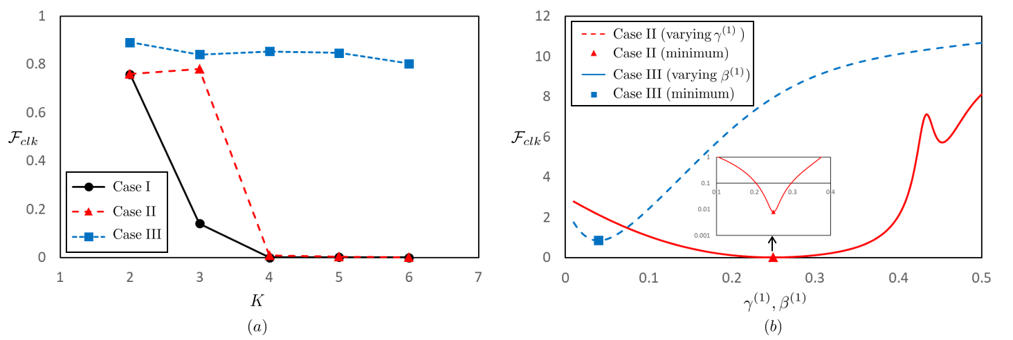
Next, we investigate the effect of the number of layers on the effectiveness of the cloaking plate. We fix the outermost radius of the plate at and we plot the cloaking factor versus the number of layers for the optimized plate for the three cases (I, II, & III) in Fig. 3(a). Interestingly, when the layer number is , the cloaking factors in cases I and II become less than 0.01. However, the cloaking factor in case III does not decrease significantly and the cloaking factor remains above 0.8. As a result, varying flexural rigidity is essential for manipulating waves and creating a cloaking buoyant plate. Since the case I has a cloaking factor smaller than case II, optimizing the mass helps to achieve a better cloak, nevertheless only optimizing the mass is insufficient to realize an effective cloaking plate. To investigate the sensitivity of the cloaking factor to the flexural rigidity and mass, we calculate the cloaking factor while modulating these parameters. The sensitivity of the factor to these parameters is shown in Fig. 3(b). The result of case II against varying mass , and that of case III against varying flexural rigidity are plotted; optimum values are marked by square and triangle respectively. The inset figure shows the semi-log plot of the cloaking factor around the minimum value for case II. According to the semi-log graph, the cloaking factor for case II increases as the mass slightly changes from the optimum value. When the mass and flexural rigidity are far from the optimum values, the cloaking factors are bigger than 1.0 meaning that the structure scatters waves with an energy larger than that of the isolated cylinder. It can be concluded that the cloaking factor is sensitive to both flexural rigidity and mass of the plate and large deviation can be detrimental to the efficacy of the cloaking plate.
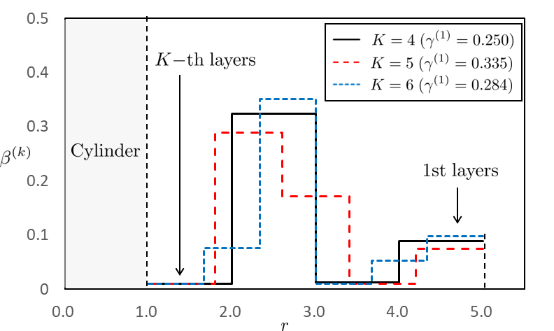
The spatial distribution of the flexural rigidity in case II is shown in Fig. 4 where it shows the structural flexural rigidity profile of the multi-layered plate. Note that is the cylinder region; the plate is at . Results of and are plotted and fix values of mass are noted in the legend. For , the plate has two sets of peaks and valleys with the first peak being larger than the second one. The values of valleys are almost at which is the lower limit of the physical parameter (see Eq. (54)). Interestingly, the rigidity profile follows a similar trend for different number of layers. The two sets of peaks and valleys are not achievable with only three number of layers, and this might be the reason why cloaking can not be achieved for (see Fig. 3(a)).
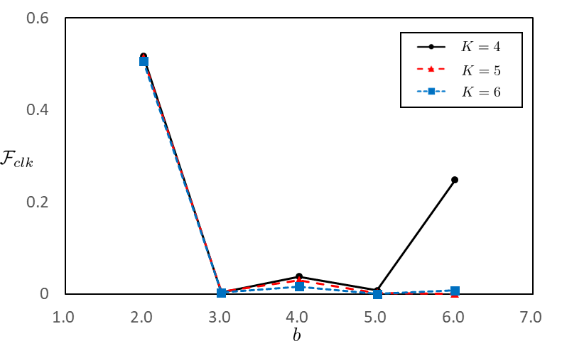
In addition to the number of layers, we analyze the influence of the outermost radius on the cloaking factor. The cloaking factor for case II against the outermost radius is shown in Fig. 5. When the outermost radius is , the factor is not fully reduced even with increasing the number of layers . The cloaking factor for and is also not small enough, while results of and are less than 0.01. When , the cloaking factors for different values of are , , and ; the use of the larger layer number helps us to achieve a smaller cloaking factor. In summary, it is observed that the size of the plate affects the cloaking factor and cloaking can not be realized using a small plate size. Additionally, using a bigger plate size does not necessarily indicate a better cloaking result. An optimized plate size exists that should be selected for efficient cloaking.
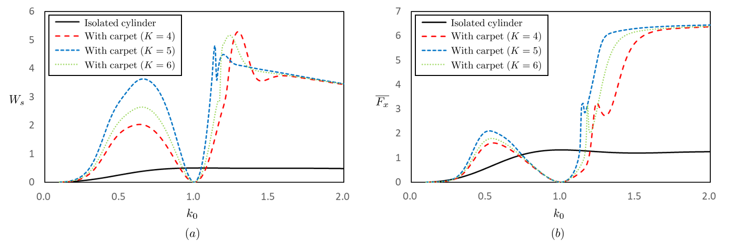
Lastly, we analyze the frequency response of the cloaking plate, i.e. the behavior of the structures for wave numbers or wave frequencies other than the value that it is optimized for. The energy of scattered-waves is shown in Fig. 6(a), and; the wave drift force acting in -direction is shown in Fig. 6(b). The result of the isolated cylinder and the results of the cylinder with the multi-layered cloak are compared. The outermost radius of the plate is fixed at , and physical parameters in case II are used. Looking at , the wave drift force of the isolated cylinder is and the cloaked wave drift forces by different are , and ; 99.9% reduction of wave drift force is achieved at most. Therefore, both energy of scattered-waves and wave drift force are dramatically reduced and become almost zero using the multi-layered cloak at the target wave number . Note that the wave drift force is the second-order force based on the law of action and reaction of wave scattering. As a result, the wave drift force is not acting on the structures if no scattered-wave is generated, or if the scattered-wave field is -symmetric as shown in Fig. 2(A). As for frequency responses, the drift force of the cloaked cylinder is smaller than that of the isolated cylinder around the target wave number with a bandwidth of (in case of ). However, these values are larger than those of the isolated cylinder outside this band, meaning that energy scattered by the structures is larger than that of the isolated cylinder. Note that the energy of scattered-waves and the wave drift force converge as and . Interestingly, using a larger number of layers does not indicate a smaller wave drift force for the frequency bands. For realizing an optimized cloak in a frequency band, a multi-objective optimization might be implemented instead of our one frequency optimization. Since we can increase the degrees of freedom for controlling wave propagation by easily increasing the number of layers in the multi-layered plate, such plate design can potentially achieve a broadband cloak from deep water waves.
6 Conclusion
We present cloaking of a bottom-mounted cylinder from water waves in deep-sea using a multi-layered elastic plate floating on the surface around the cylinder. In the governing equation of surface gravity waves, the sea bed topography and the gravitational acceleration are the only physical parameters controlling the trajectory of wave propagation; nevertheless, the effect of sea depth exponentially decreases as the depth increases, and the gravitational acceleration is physical constant. As a consequence, cloaking the offshore structure from deep water waves becomes a challenge. Here, we propose the use of a multi-layered buoyant plate to provide extra adjustable degrees of freedom for controlling wave propagation. The plate consists of concentric annular layers with isotropic and homogeneous physical parameters. This design enables easier experimental implementation. The multi-layered cloak is created based on the scattering cancellation method; the plate cancels out the scattered-waves from the cylinder. Physical parameters of each layer are optimized using an evolutionary strategy method, specifically a real-coded genetic algorithm. A numerical calculation scheme is developed using pseudo-spectral and eigenvalue matching methods, and the effectiveness of the multi-layered cloak is evaluated. The plate is designed to cloak the cylinder at the specific wave number. We vary different parameters of the buoyant cloaking plate and analyzed their effects on the cloaking factor. We show that an optimum cloaking size and the number of layers exist for maximally increasing the efficiency of the cloak. We further address the sensitivity of the cloak to changes in the wave frequency and show an optimum working bandwidth exists. Since the reduction of the wave drift force is important for practical applications, we show that our proposed cloak has 99.9% reduction of wave drift force at most. We believe that our proposed cloak has potential real-world applications in the fields of offshore industries to protect offshore structures.
References
- Alù & Engheta (2005) Alù, Andrea & Engheta, Nader 2005 Achieving transparency with plasmonic and metamaterial coatings. Physical Review E 72 (1), 016623.
- Berraquero et al. (2013) Berraquero, C.P.and Maurel, A., Petitjeans, P. & Pagneux, V. 2013 Experimental realization of a water-wave metamaterial shifter. Physical Review E 88 (5), 051002.
- Brûlé et al. (2014) Brûlé, S., Javelaud, E. H., Enoch, S. & Guenneau, S. 2014 Experiments on seismic metamaterials: Molding surface waves. Physical Review Letters 112, 133901.
- Chen & Chan (2007) Chen, H. & Chan, C.T. 2007 Acoustic cloaking in three dimensions using acoustic metamaterials. Applied Physics Letters 91 (18), 183518, arXiv: https://doi.org/10.1063/1.2803315.
- Cummer & Schurig (2007) Cummer, S. A. & Schurig, D. 2007 One path to acoustic cloaking. New Journal of Physics 9 (3), 45.
- Darabi et al. (2018a) Darabi, A., Zareei, A., Alam, M. R. & Leamy, M. J. 2018a Broadband bending of flexural waves: acoustic shapes and patterns. Scientific reports 8 (1), 1–7.
- Darabi et al. (2018b) Darabi, A., Zareei, A., Alam, M. R. & Leamy, M. J. 2018b Experimental demonstration of an ultrabroadband nonlinear cloak for flexural waves. Physical review letters 121 (17), 174301.
- Dupont et al. (2016) Dupont, G.and Guenneau, S., Kimmoun, O., Molin, B. & Enoch, S. 2016 Cloaking a vertical cylinder via homogenization in the mild-slope equation. Journal of Fluid Mechanics 796.
- Farhat et al. (2008) Farhat, M., Enoch, S., Guenneau, S. & Movchan, A. B. 2008 Broadband cylindrical acoustic cloak for linear surface waves in a fluid. Physical Review Letters 101, 134501.
- Farhat & Enoch (2009) Farhat, M. Guenneau, S. & Enoch, S. 2009 Ultrabroadband elastic cloaking in thin plates. Physical Review Letters 103, 024301.
- Fox & Squire (1994) Fox, C. & Squire, V. A. 1994 On the oblique reflexion and transmission of ocean waves at shore fast sea ice. Philosophical Transactions of the Royal Society of London. Series A: Physical and Engineering Sciences 347 (1682), 185–218.
- Guild et al. (2011) Guild, Matthew D, Alu, Andrea & Haberman, Michael R 2011 Cancellation of acoustic scattering from an elastic sphere. The Journal of the Acoustical Society of America 129 (3), 1355–1365.
- Huang et al. (2014) Huang, X., Zhong, S. & Liu, X. 2014 Acoustic invisibility in turbulent fluids by optimised cloaking. Journal of Fluid Mechanics 749, 460–477.
- Iida & Kashiwagi (2018) Iida, T. & Kashiwagi, M. 2018 Small water channel network for designing wave fields in shallow water. Journal of Fluid Mechanics 849, 90–110.
- Iida et al. (2014) Iida, T., Kashiwagi, M. & He, G. 2014 Numerical confirmation of cloaking phenomenon on an array of floating bodies and reduction of wave drift force. International Journal of Offshore and Polar Engineering 24 (4), 241–246.
- Iida et al. (2016) Iida, T., Kashiwagi, M. & Miki, M. 2016 Wave pattern in cloaking phenomenon around a body surrounded by multiple vertical circular cylinders. International Journal of Offshore and Polar Engineering 26 (1), 13–19.
- Kashiwagi et al. (2005) Kashiwagi, M., Endo, K. & Yamaguchi, H. 2005 Wave drift forces and moments on two ships arranged side by side in waves. Ocean engineering 32 (5–6), 529–555.
- Kashiwagi & Yoshida (2001) Kashiwagi, M. & Yoshida, S. 2001 Wave drift force and moment on vlfs supported by a great number of floating columns. International Journal of Offshore and Polar Engineering 11 (3).
- Loukogeorgaki & Kashiwagi (2019) Loukogeorgaki, E. & Kashiwagi, M. 2019 Minimization of drift force on a floating cylinder by optimizing the flexural rigidity of a concentric annular plate. Applied Ocean Research 85, 136–150.
- Maruo (1960) Maruo, H. 1960 The drift on a body floating in waves. Journal of Ship Research 4 (3), 1–10.
- Meylan (2002) Meylan, M.H. 2002 Wave response of an ice floe of arbitrary geometry. Journal of Geophysical Research 107 (C1).
- Newman (1977) Newman, J. N. 1977 Marine hydrodynamics. The MIT press .
- Newman (2014) Newman, J. N. 2014 Cloaking a circular cylinder in water waves. European Journal of Mechanics - B/Fluids 47, 145–150.
- Ono et al. (1999) Ono, I., Kita, H. & Kobayashi, S. 1999 A robust real-coded genetic algorithm using unimodal normal distribution crossover augmented by uniform crossover: Effects of self-adaptation of crossover probabilities. Proceedings of the 1st Annual Conference on Genetic and Evolutionary Computation 1, 496–503.
- Pendry et al. (2006) Pendry, J. B., Schurig, D. & Smith, D. R. 2006 Controlling electromagnetic fields. Science 312 (5781), 1780–1782, arXiv: http://science.sciencemag.org/content/312/5781/1780.full.pdf.
- Peter et al. (2004) Peter, M. A., Meylan, M. H. & Chung, H. 2004 Wave scattering by a circular elastic plate in water of finite depth: a closed form solution. International Journal of Offshore and Polar Engineering 14 (2).
- Porter (2011) Porter, R. 2011 Cloaking of a cylinder in waves. Proceedings of 26th International Workshop on Water Waves and Floating Bodies, Athens, Greece .
- Porter & Newman (2014) Porter, R. & Newman, J. N. 2014 Cloaking of a vertical cylinder in waves using variable bathymetry. Journal of Fluid Mechanics 750, 124–143.
- Schurig et al. (2006) Schurig, D., Mock, J. J., Justice, B.J., Cummer, S.A., Pendry, J.B., Starr, A.F. & Smith, D. R. 2006 Metamaterial electromagnetic cloak at microwave frequencies. Science 314, 977–980.
- Stenger & Wegener (2012) Stenger, N.and Wilhelm, M. & Wegener, M. 2012 Experiments on elastic cloaking in thin plates. Physical Review Letters 108, 014301.
- Zareei & Alam (2015) Zareei, A. & Alam, M. R. 2015 Cloaking in shallow-water waves via nonlinear medium transformation. Journal of Fluid Mechanics 778, 273–287.
- Zareei & Alam (2017) Zareei, A. & Alam, M. R. 2017 Broadband cloaking of flexural waves. Physical Review E 95 (6), 063002.
- Zareei et al. (2018) Zareei, A., Darabi, A., Leamy, M. J. & Alam, M. R. 2018 Continuous profile flexural grin lens: Focusing and harvesting flexural waves. Applied Physics Letters 112 (2), 023901.
- Zhang et al. (2019) Zhang, Z., He, G., Wang, Z., Liu, S., Gou, Y. & Liu, Y. 2019 Numerical and experimental studies on cloaked arrays of truncated cylinders under different wave directions. Ocean Engineering 183, 305–317.
Appendix A Details of boundary conditions
In the following we list the details of all boundary conditions that are used:
-
•
Matching conditions of the velocity potential between the free surface and the structure ( equations):
(58) -
•
Matching conditions of the radial derivative of the velocity potential between the free surface and the structure ( equations):
(62) -
•
Matching conditions of the velocity potential between adjacent layers ( equations):
(67) -
•
Matching conditions of the radial derivative of the velocity potential between adjacent layers ( equations):
(72) -
•
No flux conditions at the surface of the cylinder ( equations):
(76) -
•
Matching conditions of the wave elevation between adjacent layers ( equations):
(81) where
-
•
Matching conditions of the radial derivative of the wave elevation between adjacent layers ( equations):
(86) -
•
Matching conditions of the bending moment between adjacent layers ( equations):
(87) -
•
Matching conditions of the shear force between adjacent layers ( equations):
(88) -
•
Free-free beam conditions; zero bending moment and shear force (4 equations):
(93)