Deep Variational Multivariate Information Bottleneck -
A Framework for Variational Losses
Abstract
Variational dimensionality reduction methods are known for their high accuracy, generative abilities, and robustness. We introduce a framework to unify many existing variational methods and design new ones. The framework is based on an interpretation of the multivariate information bottleneck, in which an encoder graph, specifying what information to compress, is traded-off against a decoder graph, specifying a generative model. Using this framework, we rederive existing dimensionality reduction methods including the deep variational information bottleneck and variational auto-encoders. The framework naturally introduces a trade-off parameter extending the deep variational CCA (DVCCA) family of algorithms to beta-DVCCA. We derive a new method, the deep variational symmetric informational bottleneck (DVSIB), which simultaneously compresses two variables to preserve information between their compressed representations. We implement these algorithms and evaluate their ability to produce shared low dimensional latent spaces on Noisy MNIST dataset. We show that algorithms that are better matched to the structure of the data (in our case, beta-DVCCA and DVSIB) produce better latent spaces as measured by classification accuracy, dimensionality of the latent variables, and sample efficiency. We believe that this framework can be used to unify other multi-view representation learning algorithms and to derive and implement novel problem-specific loss functions.
Keywords: Information Bottleneck, Symmetric Information Bottleneck, Variational Methods, Generative Models, Dimensionality Reduction, Data Efficiency
1 Introduction
Large dimensional multi-modal datasets are abundant in multimedia systems utilized for language modeling (Xu et al., 2016; Zhou et al., 2018; Rohrbach et al., 2017; Sanabria et al., 2018; Goyal et al., 2017; Wang et al., 2018; Hendrycks et al., 2020), neural control of behavior studies (Steinmetz et al., 2021; Urai et al., 2022; Krakauer et al., 2017; Pang et al., 2016), multi-omics approaches in systems biology (Clark et al., 2013; Zheng et al., 2017; Svensson et al., 2018; Huntley et al., 2015; Lorenzi et al., 2018), and many other domains. Such data come with the curse of dimensionality, making it hard to learn the relevant statistical correlations from samples. The problem is made even harder by the data often containing information that is irrelevant to the specific questions one asks. To tackle these challenges, a myriad of dimensionality reduction (DR) methods have emerged. By preserving certain aspects of the data while discarding the remainder, DR can decrease the complexity of the problem, yield clearer insights, and provide a foundation for more refined modeling approaches.
DR techniques span linear methods like Principal Component Analysis (PCA) (Hotelling, 1933), Partial Least Squares (PLS) (Wold et al., 2001), Canonical Correlations Analysis (CCA) (Hotelling, 1936), and regularized CCA (Vinod, 1976; Årup Nielsen et al., 1998), as well as nonlinear approaches, including Autoencoders (AE) (Hinton and Salakhutdinov, 2006), Deep CCA (Andrew et al., 2013), Deep Canonical Correlated AE (Wang et al., 2015), Correlational Neural Networks (Chandar et al., 2016), Deep Generalized CCA (Benton et al., 2017), and Deep Tensor CCA (Wong et al., 2021). Of particular interest to us are variational methods, such as Variational Autoencoders (VAE) (Kingma and Welling, 2014), beta-VAE (Higgins et al., 2016), Joint Multimodal VAE (JMVAE) (Suzuki et al., 2016), Deep Variational CCA (DVCCA) (Wang et al., 2016), Deep Variational Information Bottleneck (DVIB) (Alemi et al., 2017), Variational Mixture-of-experts AE (Shi et al., 2019), and Multiview Information Bottleneck (Federici et al., 2020b). These DR methods use deep neural networks and variational approximations to learn robust and accurate representations of the data, while, at the same time, often serving as generative models for creating samples from the learned distributions.
There are many theoretical derivations and justifications for variational DR methods (Kingma and Welling, 2014; Higgins et al., 2016; Suzuki et al., 2016; Wang et al., 2016; Karami and Schuurmans, 2021; Qiu et al., 2022; Alemi et al., 2017; Bao, 2021; Lee and Van der Schaar, 2021; Wang et al., 2019; Wan et al., 2021; Federici et al., 2020a; Huang et al., 2022; Hu et al., 2020). This diversity of derivations, while enabling adaptability, often leaves researchers with no principled ways for choosing a method for a particular application, for designing new methods with distinct assumptions, or for comparing methods to each other.
Here, we introduce the Deep Variational Multivariate Information Bottleneck (DVMIB) framework, offering a unified mathematical foundation for many variational DR methods. Our framework is grounded in the multivariate information bottleneck loss function (Tishby et al., 2000; Friedman et al., 2013). This loss, amenable to approximation through upper and lower variational bounds, provides a system for implementing diverse DR variants using deep neural networks. We demonstrate the framework’s efficacy by deriving the loss functions of many existing variational DR methods starting from the same principles. Furthermore, our framework naturally allows the adjustment of trade-off parameters, leading to generalizations of these existing methods. For instance, we generalize DVCCA to -DVCCA. The framework further allows us to introduce and implement in software novel DR methods. We view the DVMIB framework, with its uniform information bottleneck language, conceptual clarity of translating statistical dependencies in data via graphical models of encoder and decoder structures into variational losses, the ability to unify existing approaches, and easy adaptability to new scenarios as one of the main contributions of our work.
Beyond its unifying role, our framework offers a principled approach for deriving problem-specific loss functions using domain-specific knowledge. Thus, we anticipate its application for multi-view representation learning across diverse fields. To illustrate this, we use the framework to derive a novel dimensionality reduction method, the Deep Variational Symmetric Information Bottleneck (DVSIB), which compresses two random variables into two distinct latent variables that are maximally informative about one another. This new method produces better representations of classic datasets than previous approaches. The introduction of DVSIB is another major contribution of our paper.
In summary, our paper makes the following contributions to the field:
-
1.
Introduction of the Variational Multivariate Information Bottleneck Framework: We provide both intuitive and mathematical insights into this framework, establishing a robust foundation for further exploration.
-
2.
Rederivation and Generalization of Existing Methods within a Common Framework: We demonstrate the versatility of our framework by systematically rederiving and generalizing various existing methods from the literature, showcasing the framework’s ability to unify diverse approaches.
-
3.
Design of a Novel Method — Deep Variational Symmetric Information Bottleneck (DVSIB): Employing our framework, we introduce DVSIB as a new method, contributing to the growing repertoire of techniques in variational dimensionality reduction. The method constructs high-accuracy latent spaces from substantially fewer samples than comparable approaches.
The paper is structured as follows. First, we introduce the underlying mathematics and the implementation of the DVMIB framework. We then explain how to use the framework to generate new DR methods. In Tbl. 1, we present several known and newly derived variational methods, illustrating how easily they can be derived within the framework. As a proof of concept, we then benchmark simple computational implementations of methods in Tbl. 1 against the Noisy MNIST dataset. Appendices present detailed treatment of all terms in variational losses in our framework, discussion of multi-view generalizations, and more details —including visualizations— of the performance of many methods on the Noisy MNIST.
2 Multivariate Information Bottleneck Framework
We represent DR problems similar to the Multivariate Information Bottleneck (MIB) of Friedman et al. (2013), which is a generalization of the more traditional Information Bottleneck algorithm (Tishby et al., 2000) to multiple variables. The reduced representation is achieved as a trade-off between two Bayesian networks. Bayesian networks are directed acyclic graphs that provide a factorization of the joint probability distribution, , where is the set of parents of in graph . The multiinformation (Studenỳ and Vejnarová, 1998) of a Bayesian network is defined as the Kullback-Leibler divergence between the joint probability distribution and the product of the marginals, and it serves as a measure of the total correlations among the variables, . For a Bayesian network, the multiinformation reduces to the sum of all the local informations (Friedman et al., 2013).
The first of the Bayesian networks is an encoder (compression) graph, which models how compressed (reduced, latent) variables are obtained from the observations. The second network is a decoder graph, which specifies a generative model for the data from the compressed variables, i.e., it is an alternate factorization of the distribution. In MIB, the information of the encoder graph is minimized, ensuring strong compression (corresponding to the approximate posterior). The information of the decoder graph is maximized, promoting the most accurate model of the data (corresponding to maximizing the log-likelihood). As in IB (Tishby et al., 2000), the trade-off between the compression and reconstruction is controlled by a trade-off parameter :
| (1) |
In this work, our key contribution is in writing an explicit variational loss for typical information terms found in both the encoder and the decoder graphs. All terms in the decoder graph use samples of the compressed variables as determined from the encoder graph. If there are two terms that correspond to the same information in Eq. (1), one from each of the graphs, they do not cancel each other since they correspond to two different variational expressions. For pedagogical clarity, we do this by first analyzing the Symmetric Information Bottleneck (SIB), a special case of MIB. We derive the bounds for three types of information terms in SIB, which we then use as building blocks for all other variational MIB methods in subsequent Sections.
2.1 Deep Variational Symmetric Information Bottleneck
The Deep Variational Symmetric Information Bottleneck (DVSIB) simultaneously reduces a pair of datasets and into two separate lower dimensional compressed versions and . These compressions are done at the same time to ensure that the latent spaces are maximally informative about each other. The joint compression is known to decrease data set size requirements compared to individual ones (Martini and Nemenman, 2023). Having distinct latent spaces for each modality usually helps with interpretability. For example, could be the neural activity of thousands of neurons, and could be the recordings of joint angles of the animal. Rather than one latent space representing both, separate latent spaces for the neural activity and the joint angles are sought. By maximizing compression as well as , one constructs the latent spaces that capture only the neural activity pertinent to joint movement and only the movement that is correlated with the neural activity (cf. Pang et al. (2016)). Many other applications could benefit from a similar DR approach.
In Fig. 1, we define two Bayesian networks for DVSIB, and . encodes the compression of to and to . It corresponds to the factorization and the resultant . The term does not depend on the compressed variables, does not affect the optimization problem, and hence is discarded in what follows. represents a generative model for and given the compressed latent variables and . It corresponds to the factorization and the resultant . Combing the informations from both graphs and using Eq. (1), we find the SIB loss:
| (2) |
Note that information in the encoder terms is minimized, and information in the decoder terms is maximized. Thus, while it is tempting to simplify Eq. (2) by canceling and , this would be a mistake. Indeed, these terms come from different factorizations: the encoder corresponds to learning , and the decoder to .
While the DVSIB loss may appear similar to previous models, such as MultiView Information Bottleneck (MVIB) (Federici et al., 2020b) and Barlow Twins (Zbontar et al., 2021), it is distinct both conceptually and in practice. For example, MVIB aims to generate latent variables that are as similar to each other as possible, sharing the same domain. DVSIB, however, endeavors to produce distinct latent representations, which could potentially have different units or dimensions, while maximizing mutual information between them. Barlow Twins architecture on the other hand appears to have two latent subspaces while in fact they are one latent subspace that is being optimized by a regular information bottleneck.
We now follow a procedure and notation similar to Alemi et al. (2017) and construct variational bounds on all and terms. Terms without leaf nodes, i. e., , require new approaches.
2.2 Variational bounds on DVSIB encoder terms
The information corresponds to compressing the random variable to . Since this is an encoder term, it needs to be minimized in Eq. (2). Thus, we seek a variational bound , where is the variational version of , which can be implemented using a deep neural network. We find by using the positivity of the Kullback–Leibler divergence. We make be a variational approximation to . Then , so that . Thus, . We then add to both sides and find:
| (3) |
We further simplify the variational loss by approximating , so that:
| (4) |
The term can be treated in an analogous manner, resulting in:
| (5) |
2.3 Variational bounds on DVSIB decoder terms
The term corresponds to a decoder of from the compressed variable . It is maximized in Eq. (2). Thus, we seek its variational version , such that . Here, will serve as a variational approximation to . We use the positivity of the Kullback-Leibler divergence, , to find . This gives . We add the entropy of to both sides to arrive at the variational bound:
| (6) |
We further simplify by replacing by samples, and using the that we learned previously from the encoder:
| (7) |
Here does not depend on and, therefore, can be dropped from the loss. The variational version of is obtained analogously:
| (8) |
2.4 Variational Bounds on decoder terms not on a leaf - MINE
The variational bound above cannot be applied to the information terms that do not contain leaves in . For SIB, this corresponds to the term. This information is maximized. To find a variational bound such that , we use the MINE mutual information estimator (Belghazi et al., 2018), which samples both and from their respective variational encoders. Other mutual information estimators, such as (Poole et al., 2019), can be used as long as they are differentiable. Other estimators might be better suited for different problems, but for our current application, was sufficient. We variationally approximate as , where is the normalization factor. Here is parameterized by a neural network that takes in samples of the latent spaces and and returns a single number. We again use the positivity of the Kullback-Leibler divergence, , which implies . Subtracting from both sides, we find:
| (9) |
2.5 Parameterizing the distributions and the reparameterization trick
, , and do not depend on and and are dropped from the loss. Further, we can use any ansatz for the variational distributions we introduced. We choose parametric probability distribution families and learn the nearest distribution in these families consistent with the data. We assume is a normal distribution with mean and a diagonal variance . We learn the mean and the log variance as neural networks. We also assume that is normal with a mean and a unit variance. In principle, we could also learn the variance for this distribution, but practically we did not find the need for that, and the approach works well as is. Finally, we assume that is a standard normal distribution. We use the reparameterization trick to produce samples of from , where is drawn from a standard normal distribution (Kingma and Welling, 2014). We choose the same types of distributions for the corresponding terms.
To sample from we use , where and , and is the number of new samples being generated. To sample from , we generate samples from and scramble the generated entries and , destroying all correlations. With this, the components of the loss function become
| (10) | ||||
| (11) | ||||
| (12) |
where , is the dimension of , and the corresponding terms for are similar. Combining these terms results in the variational loss for DVSIB:
| (13) |
| Method Description | ||
|---|---|---|
|
beta-VAE (Kingma and Welling, 2014; Higgins et al., 2016): Two independent Variational Autoencoder (VAE) models trained, one for each view, and (only graphs/loss shown).
|
|
|
|
DVIB (Alemi et al., 2017): Two bottleneck models trained, one for each view, and , using the other view as the supervising signal. (Only graphs/loss shown).
|
|
|
|
beta-DVCCA: Similar to DVIB (Alemi et al., 2017), but with reconstruction of both views. Two models trained, compressing either or , while reconstructing both and . (Only graphs/loss shown).
DVCCA (Wang et al., 2016):-DVCCA with . |
|
|
|
beta-joint-DVCCA: A single model trained using a concatenated variable , learning one latent representation .
joint-DVCCA (Wang et al., 2016): -jDVCCA with . |
|
|
|
beta-DVCCA-private: Two models trained, compressing either or , while reconstructing both and , and simultaneously learning private information and . (Only graphs/loss shown).
DVCCA-private (Wang et al., 2016): -DVCCA-p with . |
|
|
|
beta-joint-DVCCA-private: A single model trained using a concatenated variable , learning one latent representation , and simultaneously learning private information and .
joint-DVCCA-private(Wang et al., 2016): -jDVCCA-p with . |
|
|
|
DVSIB: A symmetric model trained, producing and .
|
|
|
|
DVSIB-private: A symmetric model trained, producing and , while simultaneously learning private information and .
|
|
|
3 Deriving other DR methods
The variational bounds used in DVSIB can be used to implement loss functions that correspond to other encoder-decoder graph pairs and hence to other DR algorithms. The simplest is the beta variational auto-encoder. Here consists of one term: compressed into . Similarly consists of one term: decoded from (see Table 1). Using this simple set of Bayesian networks, we find the variational loss:
| (14) |
Both terms in Eq. (14) are the same as Eqs. (10, 11) and can be approximated and implemented by neural networks.
Similarly, we can re-derive the DVCCA family of losses (Wang et al., 2016). Here is compressed into . reconstructs both and from the same compressed latent space . In fact, our loss function is more general than the DVCCA loss and has an additional compression-reconstruction trade-off parameter . We call this more general loss -DVCCA, and the original DVCCA emerges when :
| (15) |
Using the same library of terms as we found in DVSIB, Eqs. (10, 11), we find:
| (16) |
This is similar to the loss function of the deep variational CCA (Wang et al., 2016), but now it has a trade-off parameter . It trades off the compression into against the reconstruction of and from the compressed variable .
4 Results


To test our methods, we created a dataset inspired by the noisy MNIST dataset (LeCun et al., 1998; Wang et al., 2015, 2016), consisting of two distinct views of data, both with dimensions of pixels, cf. Fig. 2. The first view comprises the original image randomly rotated by an angle uniformly sampled between and and scaled by a factor uniformly distributed between and . The second view consists of the original image with an added background Perlin noise (Perlin, 1985) with the noise factor uniformly distributed between and . Both image intensities are scaled to the range of . The dataset was shuffled within labels, retaining only the shared label identity between two images, while disregarding the view-specific details, i.e., the random rotation and scaling for , and the correlated background noise for . The dataset, totaling images, was partitioned into training (), testing (), and validation () subsets. Visualization via t-SNE (Hinton and Roweis, 2002) plots of the original dataset suggest poor separation by digit, and the two digit views have diverse correlations, making this a sufficiently hard problem.
The DR methods we evaluated include all methods from Tbl. 1. PCA and CCA (Hotelling, 1933, 1936) served as a baseline for linear dimensionality reduction. Multi-view Information Bottleneck Federici et al. (2020b) was included for a specific comparison with DVSIB (see Appendix C). We emphasize that none of the algorithms were given labeled data. They had to infer compressed latent representations that presumably should cluster into ten different digits based simply on the fact that images come in pairs, and the (unknown) digit label is the only information that relates the two images.
Each method was trained for 100 epochs using fully connected neural networks with layer sizes , where is the latent dimension size, employing ReLU activations for the hidden layers. The input dimension was either the size of (784) or the size of the concatenated (1568). The last two layers of size represented the means and learned. For the decoders, we employed regular decoders, fully connected neural networks with layer sizes , using ReLU activations for the hidden layers and sigmoid activation for the output layer. Again, the output dimension could either be the size of (784) or the size of the concatenated (1568). The latent dimension could be or for regular decoders, or or for decoders with private information. Additionally, another decoder denoted as decoder_MINE, based on the MINE estimator for estimating , was used in DVSIB and DVSIB with private information. The decoder_MINE is a fully connected neural network with layer sizes and ReLU activations for the hidden layers. Optimization was conducted using the ADAM optimizer with default parameters.
| Method | Acc. % | |||||
|---|---|---|---|---|---|---|
| Baseline | 90.8 | 784† | - | - | - | 0.1 |
| PCA | 90.5 | 256 | [64,256*] | - | - | 1 |
| CCA | 85.7 | 256 | [32,256*] | - | - | 10 |
| -VAE | 96.3 | 256 | [64,256*] | 32 | [2,1024*] | 10 |
| DVIB | 90.4 | 256 | [16,256*] | 512 | [8,1024*] | 0.003 |
| DVCCA | 89.6 | 128 | [16,256*] | 1† | - | 31.623 |
| -DVCCA | 95.4 | 256 | [64,256*] | 16 | [2,1024*] | 10 |
| DVCCA-p | 92.1 | 16 | [16,256*] | 1† | - | 0.316 |
| -DVCCA-p | 95.5 | 16 | [4,256*] | 1024 | [1,1024*] | 0.316 |
| MVIB | 97.7 | 8 | [4,64] | 1024 | [128,1024*] | 0.01 |
| DVSIB | 97.8 | 256 | [8,256*] | 128 | [2,1024*] | 3.162 |
| DVSIB-p | 97.8 | 256 | [8,256*] | 32 | [2,1024*] | 10 |
| jBaseline | 91.9 | 1568† | - | - | - | 0.003 |
| jDVCCA | 92.5 | 256 | [64,265*] | 1† | - | 10 |
| -jDVCCA | 96.7 | 256 | [16,265*] | 256 | [1,1024*] | 1 |
| jDVCCA-p | 92.5 | 64 | [32,265*] | 1† | - | 10 |
| -jDVCCA-p | 92.7 | 256 | [4,265*] | 2 | [1,1024*] | 10 |


To evaluate the methods, we trained them on the training portions of and without exposure to the true labels. Subsequently, we utilized the trained encoders to compute , , and on the respective datasets. To assess the quality of the learned representations, we revealed the labels of and trained a linear SVM classifier with and . Fine-tuning of the classifier was performed to identify the optimal SVM slack parameter ( value), maximizing accuracy on . This best classifier was then used to predict , yielding the reported accuracy. We also conducted classification experiments using fully connected neural networks, with detailed results available in the Appendix D. For both SVM and the fully connected network, we find the baseline accuracy on the original training data and labels and , fine-tuning with the test datasets, and reporting the results of the validation datasets. Using Linear SVM enables us to assess the linear separability of the clusters of and obtained through the DR methods. While neural networks excel at uncovering nonlinear relationships that could result in higher classification accuracy, the comparison with a linear SVM establishes a level playing field. It ensures a fair comparison among different methods and is independent of the success of the classifier used for comparison in detecting nonlinear features in the data, which might have been missed by the DR methods. Here, we focus on the results of the datasets (MNIST with correlated noise background); results for are in the Appendix D. A parameter sweep was performed to identify optimal values, ranging from to dimensions on scale, as well as optimal values, ranging from to . For methods with private information, and were varied from to . The highest accuracy is reported in Tbl. 2, along with the optimal parameters used to obtain this accuracy. Additionally, for every method we find the range of and the dimensionality of the latent variable that gives 95% of the method’s maximum accuracy. If the range includes the limits of the parameter, this is indicated by an asterisk.
Figure 3 shows a t-SNE plot of DVSIB’s latent space, , colored by the identity of digits. The resulting latent space has 10 clusters, each corresponding to one digit. The clusters are well separated and interpretable. Further, DVSIB’s latent space provides the best classification of digits using a linear method such as an SVM showing the latent space is linearly separable. DVSIB maximum classification accuracy obtained for the linear SVM is 97.8%. Crucially, DVSIB maintains accuracy of at least 92.9% (95% of 97.8%) for and . This accuracy is high compared to other methods and has a large range of hyperparameters that maintain its ability to correctly capture information about the identity of the shared digit. DVSIB is a generative method, we have provided sample generated digits from the decoders that were trained from the model graph.

In Fig. 4, we show the highest SVM classification accuracy curves for each method. DVSIB and DVSIB-private tie for the best classification accuracy for . Together with -DVCCA-private they have the highest accuracy for all dimensions of the latent space, . In theory, only one dimension should be needed to capture the identity of a digit, but our data sets also contain information about the rotation and scale for and the strength of the background noise for . should then need at least two latent dimensions to be reconstructed and should need at least three. Since DVSIB, DVSIB-private, and -DVCCA-private performed with the best accuracy starting with the smallest , we conclude that methods with the encoder-decoder graphs that more closely match the structure of the data produce higher accuracy with lower dimensional latent spaces.
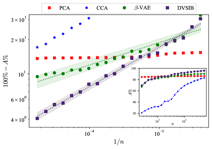
Next, in Fig. 5, we compare the sample training efficiency of DVSIB and -VAE by training new instances of these methods on a geometrically increasing number of samples , consisting of 20 subsamples of the full training data () to get (), where each larger subsample includes the previous one. Each method was trained for 60 epochs, and we used (as defined by the DVMIB framework). Further, all reported results are with the latent space size . We explored other numbers of training epochs and latent space dimensions (see Appendix D.6), but did not observe qualitative differences. We follow the same procedure as outlined earlier, using the 20 trained encoders for each method to compute , , and for the training, test, and validation datasets. As before, we then train and evaluate the classification accuracy of SVMs for the representation learned by each method. Fig. 5, inset, shows the classification accuracy of each method as a function of the number of samples used in training. Again, CCA and PCA serve as linear methods baselines. PCA is able to capture the linear correlations in the dataset consistently, even at low sample sizes. However, it is unable to capture the nonlinearities of the data, and its accuracy does not improve with the sample size. Because of the iterative nature of the implementation of the PCA algorithm (Pedregosa et al., 2011), it is able to capture some linear correlations in a relatively low number of dimensions, which are sufficiently sampled even with small-sized datasets. Thus the accuracy of PCA barely depends on the training set size. CCA, on the other hand, does not work in the under-sampled regime (see Abdelaleem et al. (2023) for discussion of this). DVSIB performs uniformly better, at all training set sizes, than the -VAE. Furthermore, DVSIB improves its quality faster, with a different sample size scaling. Specifically, DVSIB and -VAE accuracy (, measured in percent) appears to follow the scaling form , where is a constant, and the scaling exponent for DVSIB, and for -VAE. We illustrate this scaling in Fig. 5 by plotting a log-log plot of vs and observing a linear relationship.
5 Conclusion
We developed an MIB-based framework for deriving variational loss functions for DR applications. We demonstrated the use of this framework by developing a novel variational method, DVSIB. DVSIB compresses the variables and into latent variables and respectively, while maximizing the information between and . The method generates two distinct latent spaces—a feature highly sought after in various applications—but it accomplishes this with superior data efficiency, compared to other methods. The example of DVSIB demonstrates the process of deriving variational bounds for terms present in all examined DR methods. A comprehensive library of typical terms is included in Appendix A for reference, which can be used to derive additional DR methods. Further, we (re)-derive several DR methods, as outlined in Table 1. These include well-known techniques such as -VAE, DVIB, DVCCA, and DVCCA-private. MIB naturally introduces a trade-off parameter into the DVCCA family of methods, resulting in what we term the -DVCCA DR methods, of which DVCCA is a special case. We implement this new family of methods and show that it produces better latent spaces than DVCCA at , cf. Tbl. 2.
We observe that methods that more closely match the structure of dependencies in the data can give better latent spaces as measured by the dimensionality of the latent space and the accuracy of reconstruction (see Figure 4). This makes DVSIB, DVSIB-private, and -DVCCA-private perform the best. DVSIB and DVSIB-private both have separate latent spaces for and . The private methods allow us to learn additional aspects about and that are not important for the shared digit label, but allow reconstruction of the rotation and scale for and the background noise of . We also found that DVSIB can make more efficient use of data when producing latent spaces as compared to -VAEs and linear methods.
Our framework may be extended beyond variational approaches. For instance, in the deterministic limit of VAE, autoencoders can be retrieved by defining the encoder/decoder graphs as nonlinear neural networks and . Additionally, linear methods like CCA can be viewed as special cases of the information bottleneck (Chechik et al., 2003) and hence must follow from our approach. Similarly, by using specialized encoder and decoder neural networks, e.g., convolutional ones, our framework can implement symmetries and other constraints into the DR process. Overall, the framework serves as a versatile and customizable toolkit, capable of encompassing a wide spectrum of dimensionality reduction methods. With the provided tools and code, we aim to facilitate the adaptation of the approach to diverse problems.
Acknowledgments and Disclosure of Funding
EA and KMM contributed equally to this work. We thank Sean Ridout and Michael Pasek for providing feedback on the manuscript. EA and KMM also thank Ahmed Roman for useful discussions. IN is particularly grateful to the late Tali Tishby for many discussions about life, science, and information bottleneck over the years. This work was funded, in part, by NSF Grants Nos. 2010524 and 2014173, by the Simons Investigator award to IN, and the Simons-Emory International Consortium on Motor Control. We acknowledge support of our work through the use of the HyPER C3 cluster of Emory University’s AI.Humanity Initiative.
Appendix A Deriving and designing variational losses
In the next two sections, we provide a library of typical terms found in encoder graphs, Appendix A.1, and decoder graphs, AppendixA.2. In Appendix A.3, we provide examples of combining these terms to produce variational losses corresponding to beta-VAE, DVIB, beta-DVCCA, beta-DVCCA-joint, beta-DVCCA-private, DVSIB, and DVSIB-private.
A.1 Encoder graph components
We expand Sec. 2.2 and present a range of common components found in encoder graphs across various DR methods, cf. Fig. (6).
-
a.
This graph corresponds to compressing the random variable to . Variational bounds for encoders of this type were derived in the main text in Sec. 2.2 and correspond to the loss:
(17) -
b.
This type of encoder graph is similar to the first, but now with two outputs, and . This corresponds to making two encoders, one for and one for , , where
(18) (19) -
c.
This type of encoder consists of compressing and into a single variable . It corresponds to the information loss . This again has a similar encoder structure to type (a), but is replaced by a joint variable . For this loss, we find a variational version:
(20) -
d.
This final type of an encoder term corresponds to information , which is constant with respect to our minimization. In practice, we drop terms of this type.
A.2 Decoder graph components
In this section, we elaborate on the decoder graphs that happen in our considered DR methods, cf. Fig. (7).
All decoder graphs sample from their methods’ corresponding encoder graph.
-
a.
In this decoder graph, we decode from the compressed variable . Variational bounds for decoders of this type were derived in the main text, Sec. 2.3, and they correspond to the loss:
(21) where can be dropped from the loss since it doesn’t change in optimization.
-
b.
This type of decoder term is similar to that in part (a), but is decoded from two variables simultaneously. The corresponding loss term is . We find a variational loss by replacing in part (a) by :
(22) where, again, the entropy of can be dropped.
-
c.
This decoder term can be obtained by adding two decoders of type (a) together. In this case, the loss term is :
(23) and the entropy terms can be dropped, again.
-
d.
Decoders of this type were discussed in the main text in Sec. 2.4. They correspond to the information between latent variables and . We use the MINE estimator to find variational bounds for such terms:
(24)
A.3 Detailed method implementations
For completeness, we provide detailed implementations of methods outlined in Tbl. 1.
A.3.1 Beta Variational Auto-Encoder
A variational autoencoder (Kingma and Welling, 2014; Higgins et al., 2016) compresses into a latent variable and then reconstructs from the latent variable, cf. Fig. (9). The overall loss is a trade-off between the compression and the reconstruction :
| (25) |
is a constant with respect to the minimization, and it can be omitted from the loss. Similar to the main text, DVSIB case, we make ansatzes for forms of each of the variational distributions. We choose parametric distribution families and learn the nearest distribution in these families consistent with the data. Specifically, we assume is a normal distribution with mean and variance . We learn the mean and the log-variance as neural networks. We also assume that is normal with a mean and a unit variance. Finally, we assume that is drawn from a standard normal distribution. We then use the re-parameterization trick to produce samples of from , where is drawn from a standard normal distribution. Overall, this gives:
| (26) |
This is the same loss as for a beta auto-encoder. However, following the convention in the Information Bottleneck literature (Tishby et al., 2000; Friedman et al., 2013), our is the inverse of the one typically used for beta auto-encoders. A small in our case results in a stronger compression, while a large results in a better reconstruction.
A.3.2 Deep Variational Information Bottleneck
Just as in the beta auto-encoder, we immediately write down the loss function for the information bottleneck. Here, the encoder graph compresses into , while the decoder tries to maximize the information between the compressed variable and the relevant variable , cf. Fig. (9). The resulting loss function is:
| (27) |
Here the information between and does not depend on and can dropped in the optimization.
Thus the Deep Variational Information Bottleneck (Alemi et al., 2017) becomes :
| (28) |
where we dropped since it doesn’t change in the optimization.
As we have been doing before, we choose to parameterize all these distributions by Gaussians and their means and their log variances are learned by neural networks. Specifically, we parameterize , , and . Again we can use the reparameterization trick and sample from by where is drawn from a standard normal distribution.
A.3.3 Beta Deep Variational CCA
beta-DVCCA, cf. Fig. 10, is similar to the traditional information bottleneck, but now and are both used as relevance variables:
| (29) |
Using the same library of terms as before, we find:
| (30) |
This is similar to the loss function of the deep variational CCA (Wang et al., 2016), but now it has a trade-off parameter . It trades off the compression into against the reconstruction of and from the compressed variable .
A.3.4 beta joint-Deep Variational CCA
Joint deep variational CCA (Wang et al., 2016), cf. Fig. 11, compresses into one and then reconstructs the individual terms and ,
| (31) |
Using the terms we derived, the loss function is:
| (32) |
The information between and does not change under the minimization and can be dropped.
A.3.5 beta (joint) Deep Variational CCA-private
This is a generalization of the Deep Variational CCA Wang et al. (2016) to include private information, cf. Fig. 12. Here is encoded into a shared latent variable and a private latent variable . Similarly is encoded into the same shared variable and a different private latent variable . is reconstructed from and , and is reconstructed from and . In the joint version are compressed jointly in similar to the previous joint methods. What follows is the loss version of beta Deep Variational CCA-private.
| (33) |
After the usual variational manipulations, this becomes:
| (34) |
A.3.6 Deep Variational Symmetric Information Bottleneck
This has been analyzed in detail in the main text, Sec. 2.1, and will not be repeated here.
A.3.7 Deep Variational Symmetric Information Bottleneck-private
This is a generalization of the Deep Variational Symmetric Information Bottleneck to include private information. Here is encoded into a shared latent variable and a private latent variable . Similarly, is encoded into its own shared variable and a private latent variable . is reconstructed from and , and is reconstructed from and . and are constructed to be maximally informative about each another. This results in
| (35) |
After the usual variational manipulations, this becomes (see also main text):
| (36) |
where
| (37) |
Appendix B Multi-variable Losses (More than 2 Views / Variables)
It is possible to rederive several multi-variable losses that have appeared in the literature within our framework.
B.1 Multi-view Total Correlation Auto-encoder
Here we demonstrate several graphs for multi-variable losses. This first example consists of a structure, where all the views , , and are compressed into the same latent variable . The corresponding decoder produces reconstructed views from the same latent variable . This is known in the literature as a multi-view auto-encoder.
| (38) |
Using the same library of terms as before, we find:
| (39) |
B.2 Deep Variational Multimodal Information Bottlenecks
This example consists of a structure where all the views , , and are compressed into separate latent views , , and and one global shared latent variable . This structure is analogous to DVCCA-private, but it extends to three variables rather than two. It appears in the literature with slightly different variations. In the decoder graph, is reconstructed from both and , is reconstructed from both and , and is reconstructed from both and .
| (40) |
Using the same library of terms as before, we find:
| (41) |
B.3 Discussion
There exist many other structures that have been explored in the multi-view representation learning literature, including conditional VIB (Shi et al., 2019; Hwang et al., 2021), which is formulated in terms of conditional information. These types of structures are beyond the current scope of our framework. However, they could be represented by an encoder mapping from all independent views to , subtracted from another encoder mapping from the joint view to . Coupled with this would be a decoder mapping from to the independent views (or the joint view , analogous to the Joint-DVCCA). Similarly, one can use our framework to represent other multi-view approaches, or their approximations (Lee and Van der Schaar, 2021; Wan et al., 2021; Hwang et al., 2021). This underscores the breadth of methods seeking to address specific questions by exploring known or assumed statistical dependencies within data, and also the generality of our approach, which can re-derive these methods.
Appendix C Multi-view Information Bottleneck
The multiview information bottleneck (MVIB) (Federici et al., 2020b) attempts to remove redundant information between views . This is achieved with the following losses:
| (42) | ||||
| (43) |
These losses are equivalent to two deep variational information bottlenecks performed in parallel. Within our framework, the same algorithm emerges with the encoder graph that compresses into and into , while the decoder graph would reconstruct from and from .
Federici et al. (2020b) combines these two losses while enforcing the condition that and are the same. They bounded the combined loss function to obtain:
| (44) |
with and being the same latent space in this approximation. Here is the symmetrized KL divergence, corresponds to the two different views, and corresponds to their two latent, compressed representation. (Here we changed the parameter to be in front of , to be consistent with the definition of we use elsewhere in this work.) While this loss looks similar to the DVSIB loss, it is conceptually different. It attempts to produce latent variables that are as similar to one another as possible (ideally, ). In contrast, DVSIB attempts to produce different latent variables that could, in theory, have different units, dimensionalities, and domains, while still being as informative about each other as possible. For example, in the noisy MNIST, contains information about the labels, the angles, and the scale of images (all needed for reconstructing ) and no information about the noise structure. At the same time, contains information about the labels and the noise factor only (both needed to reconstruct ). See Appendix D.4 for 2-d latent spaces colored by these variables, illustrating the difference between and in DVSIB. Further, in practice, the implementation of MVIB uses the same encoder for both views of the data; this is equivalent to encoding different views using the same function and then trying to force the output to be as close as possible to each other, in contrast to DVSIB.
We evaluate MVIB on the noisy MNIST dataset and include it in Table 2. The performance is similar to that of DVSIB, but slightly worse.
Moreover, MVIB appears to be highly sensitive to parameters and training conditions. Despite employing identical initial conditions and parameters used for training other methods, the approach often experienced collapses during training, resulting in infinities. Interestingly enough, in instances where training persisted for a limited set of parameters (usually low and high ), MVIB generated good latent spaces, evidenced by their relatively high classification accuracy.
Appendix D Additional MNIST Results
In this section, we present supplementary results derived from the methods in Tbl 1.
D.1 Additional results tables for the best parameters
We report classification accuracy using SVM on data , and using neural networks on both and .
| Method | Acc. % | |||||
|---|---|---|---|---|---|---|
| Baseline | 57.8 | 784† | - | - | - | 0.01 |
| PCA | 58.0 | 256 | [32,265*] | - | - | 0.1 |
| CCA | 54.4 | 256 | [8,265*] | - | - | 0.032 |
| -VAE | 84.4 | 256 | [128,265*] | 4 | [2,8] | 10 |
| DVIB | 87.3 | 128 | [4,265*] | 512 | [8,1024*] | 0.032 |
| DVCCA | 86.1 | 256 | [64,265*] | 1† | - | 31.623 |
| -DVCCA | 88.9 | 256 | [128,265*] | 4 | [1,128] | 10 |
| DVCCA-private | 85.3 | 128 | [32,265*] | 1† | - | 31.623 |
| -DVCCA-private | 85.3 | 128 | [32,265*] | 1 | [1,8] | 31.623 |
| MVIB | 93.8 | 8 | [8,16] | 128 | [128,1024*] | 0.01 |
| DVSIB | 92.9 | 256 | [64,265*] | 256 | [4,1024*] | 1 |
| DVSIB-private | 92.6 | 256 | [32,265*] | 128 | [8,1024*] | 3.162 |
| Method | Acc. % | ||||
| Baseline | 92.8 | 784† | - | - | - |
| PCA | 97.6 | 128 | [16,256*] | - | - |
| CCA | 90.2 | 256 | [32,256*] | - | - |
| -VAE | 98.4 | 64 | [8,256*] | 64 | [2,1024*] |
| DVIB | 90.4 | 128 | [8,256*] | 1024 | [8,1024*] |
| DVCCA | 91.3 | 16 | [4,256*] | 1† | - |
| -DVCCA | 97.5 | 128 | [8,256*] | 512 | [2,1024*] |
| DVCCA-private | 93.8 | 16 | [2,256*] | 1† | - |
| -DVCCA-private | 97.5 | 256 | [2,256*] | 32 | [1,1024*] |
| MVIB | 97.5 | 16 | [8,16] | 256 | [128,1024*] |
| DVSIB | 98.3 | 256 | [4,256*] | 32 | [2,1024*] |
| DVSIB-private | 98.3 | 256 | [4,256*] | 32 | [2,1024*] |
| Baseline-joint | 97.7 | 1568† | - | - | - |
| joint-DVCCA | 93.7 | 256 | [8,256*] | 1† | - |
| -joint-DVCCA | 98.9 | 64 | [8,256*] | 512 | [2,1024*] |
| joint-DVCCA-private | 93.5 | 16 | [4,256*] | 1† | - |
| -joint-DVCCA-private | 95.6 | 32 | [4,256*] | 512 | [1,1024*] |
| Method | Acc. % | ||||
|---|---|---|---|---|---|
| Baseline | 92.8 | 784† | - | - | - |
| PCA | 91.9 | 64 | [32,256*] | - | - |
| CCA | 72.6 | 256 | [256,256*] | - | - |
| -VAE | 93.3 | 256 | [16,256*] | 256 | [2,1024*] |
| DVIB | 87.5 | 4 | [2,256*] | 1024 | [4,1024*] |
| DVCCA | 87.5 | 128 | [8,256*] | 1† | - |
| -DVCCA | 92.2 | 64 | [8,256*] | 32 | [2,1024*] |
| DVCCA-private | 88.2 | 8 | [8,256*] | 1† | - |
| -DVCCA-private | 90.7 | 256 | [4,256*] | 8 | [1,1024*] |
| MVIB | 93.6 | 8 | [8,16] | 256 | [128,1024*] |
| DVSIB | 93.9 | 128 | [8,256*] | 16 | [2,1024*] |
| DVSIB-private | 92.8 | 32 | [8,256*] | 256 | [4,1024*] |
D.2 t-SNE Embeddings at best parameters
Figures 16 and 17 display 2d t-SNE embeddings for variables and generated by various considered DR methods.


D.3 DVSIB-private reconstructions for best parameters
Figure 18 shows the t-SNE embeddings of the private latent variables constructed by DVSIB-private, colored by the digit label. To the extent that the labels do not cluster, private latent variables do not preserve the label information shared between and .


D.4 Additional results at 2 latent dimensions
We now demonstrate how different DR methods behave when the compressed variables are restricted to have not more than 2 dimensions, cf. Figs. 19, 20.


D.5 DVSIB-private reconstructions at 2 Latent Dimensions
Figure 21 shows the reconstructions of the private latent variables constructed by DVSIB-private, colored by the digit label, rotations, scales, and noise factors for (up), and (bottom). Private latent variables at 2 latent dimensions preserve a little about the label information shared between and , but clearly preserve the scale information for , even at only 2 latent dimensions.


D.6 Testing Training Efficiency
We tested an SVM’s classification accuracy for distinguishing digits based on latent subspaces created by DVSIB, -VAE, CCA, and PCA trained using different amounts of samples. Figure 5 in the main text shows the results for 60 epochs of training with latent spaces of dimension . The DVSIB and -VAE were trained with . Figure 22 shows the SVM’s classification accuracy for a range of latent dimensions (from right to left): . Additionally, it shows the results for different amounts of training time for the encoders ranging from 20 epochs (top row) to 100 epochs (bottom row). As explained in the main text, we plot a log-log graph of versus . Plotted in this way, high accuracy appears at the bottom, and large sample sizes are at the left of the plots. DVSIB, -VAE, and CCA often appear linear when plotted this way, implying that they follow the form . Steeper slopes on these plots correspond to a faster increase in the accuracy with the sample size. This parameter sweep shows that the tested methods have not had time to fully converge at low epoch numbers. Additionally, increasing the number of latent dimensions helps the SVMs untangle the non-linearities present in the data and improves the corresponding classifiers.

References
- Abdelaleem et al. (2023) Eslam Abdelaleem, Ahmed Roman, K Michael Martini, and Ilya Nemenman. Simultaneous dimensionality reduction: A data efficient approach for multimodal representations learning. arXiv preprint arXiv:2310.04458, 2023.
- Alemi et al. (2017) Alex Alemi, Ian Fischer, Josh Dillon, and Kevin Murphy. Deep variational information bottleneck. In ICLR, 2017.
- Andrew et al. (2013) Galen Andrew, Raman Arora, Jeff Bilmes, and Karen Livescu. Deep canonical correlation analysis. In Sanjoy Dasgupta and David McAllester, editors, Proceedings of the 30th International Conference on Machine Learning, volume 28 of Proceedings of Machine Learning Research, pages 1247–1255, Atlanta, Georgia, USA, 17–19 Jun 2013. PMLR.
- Bao (2021) Feng Bao. Disentangled variational information bottleneck for multiview representation learning. In Artificial Intelligence: First CAAI International Conference, CICAI 2021, Hangzhou, China, June 5–6, 2021, Proceedings, Part II 1, pages 91–102. Springer, 2021.
- Belghazi et al. (2018) Mohamed Ishmael Belghazi, Aristide Baratin, Sai Rajeshwar, Sherjil Ozair, Yoshua Bengio, Aaron Courville, and Devon Hjelm. Mutual information neural estimation. In International conference on machine learning, pages 531–540. PMLR, 2018.
- Benton et al. (2017) Adrian Benton, Huda Khayrallah, Biman Gujral, Dee Ann Reisinger, Sheng Zhang, and Raman Arora. Deep generalized canonical correlation analysis. arXiv preprint arXiv:1702.02519, 2017.
- Chandar et al. (2016) Sarath Chandar, Mitesh M. Khapra, Hugo Larochelle, and Balaraman Ravindran. Correlational neural networks. Neural Computation, 28(2):257–285, 2016. doi: 10.1162/NECO_a_00801.
- Chechik et al. (2003) Gal Chechik, Amir Globerson, Naftali Tishby, and Yair Weiss. Information bottleneck for gaussian variables. Advances in Neural Information Processing Systems, 16, 2003.
- Clark et al. (2013) Kenneth Clark, Bruce Vendt, Kirk Smith, John Freymann, Justin Kirby, Paul Koppel, Stephen Moore, Stanley Phillips, David Maffitt, Michael Pringle, et al. The cancer imaging archive (tcia): maintaining and operating a public information repository. Journal of digital imaging, 26:1045–1057, 2013.
- Federici et al. (2020a) Marco Federici, Anjan Dutta, Patrick Forré, Nate Kushman, and Zeynep Akata. Learning robust representations via multi-view information bottleneck. In 8th International Conference on Learning Representations. OpenReview. net, 2020a.
- Federici et al. (2020b) Marco Federici, Anjan Dutta, Patrick Forré, Nate Kushman, and Zeynep Akata. Learning robust representations via multi-view information bottleneck. arXiv preprint arXiv:2002.07017, 2020b.
- Friedman et al. (2013) Nir Friedman, Ori Mosenzon, Noam Slonim, and Naftali Tishby. Multivariate information bottleneck. arXiv preprint arXiv:1301.2270, 2013.
- Goyal et al. (2017) Yash Goyal, Tejas Khot, Douglas Summers-Stay, Dhruv Batra, and Devi Parikh. Making the V in VQA matter: Elevating the role of image understanding in Visual Question Answering. In Conference on Computer Vision and Pattern Recognition (CVPR), 2017.
- Hendrycks et al. (2020) Dan Hendrycks, Collin Burns, Steven Basart, Andy Zou, Mantas Mazeika, Dawn Song, and Jacob Steinhardt. Measuring massive multitask language understanding. arXiv preprint arXiv:2009.03300, 2020.
- Higgins et al. (2016) Irina Higgins, Loic Matthey, Arka Pal, Christopher Burgess, Xavier Glorot, Matthew Botvinick, Shakir Mohamed, and Alexander Lerchner. beta-vae: Learning basic visual concepts with a constrained variational framework. In International conference on learning representations, 2016.
- Hinton and Roweis (2002) Geoffrey E Hinton and Sam Roweis. Stochastic neighbor embedding. Advances in neural information processing systems, 15, 2002.
- Hinton and Salakhutdinov (2006) Geoffrey E Hinton and Ruslan Salakhutdinov. Reducing the dimensionality of data with neural networks. Science, 313(5786):504–507, 2006. doi: 10.1126/science.1127647.
- Hotelling (1933) Harold Hotelling. Analysis of a complex of statistical variables into principal components. Journal of educational psychology, 24(6):417, 1933.
- Hotelling (1936) Harold Hotelling. Relations between two sets of variates. Biometrika, 1936. doi: 10.1007/978-1-4612-4380-9_14.
- Hu et al. (2020) Shizhe Hu, Zenglin Shi, and Yangdong Ye. Dmib: Dual-correlated multivariate information bottleneck for multiview clustering. IEEE Transactions on Cybernetics, 52(6):4260–4274, 2020.
- Huang et al. (2022) Teng-Hui Huang, Aly El Gamal, and Hesham El Gamal. On the multi-view information bottleneck representation. In 2022 IEEE Information Theory Workshop (ITW), pages 37–42. IEEE, 2022.
- Huntley et al. (2015) Rachael P Huntley, Tony Sawford, Prudence Mutowo-Meullenet, Aleksandra Shypitsyna, Carlos Bonilla, Maria J Martin, and Claire O’Donovan. The goa database: gene ontology annotation updates for 2015. Nucleic acids research, 43(D1):D1057–D1063, 2015.
- Hwang et al. (2021) HyeongJoo Hwang, Geon-Hyeong Kim, Seunghoon Hong, and Kee-Eung Kim. Multi-view representation learning via total correlation objective. Advances in Neural Information Processing Systems, 34:12194–12207, 2021.
- Karami and Schuurmans (2021) Mahdi Karami and Dale Schuurmans. Deep probabilistic canonical correlation analysis. Proceedings of the AAAI Conference on Artificial Intelligence, 35(9):8055–8063, May 2021. doi: 10.1609/aaai.v35i9.16982.
- Kingma and Welling (2014) Diederik P Kingma and Max Welling. Auto-Encoding Variational Bayes. In 2nd International Conference on Learning Representations, ICLR 2014, Banff, AB, Canada, April 14-16, 2014, Conference Track Proceedings, 2014.
- Krakauer et al. (2017) John W Krakauer, Asif A Ghazanfar, Alex Gomez-Marin, Malcolm A MacIver, and David Poeppel. Neuroscience needs behavior: correcting a reductionist bias. Neuron, 93(3):480–490, 2017.
- LeCun et al. (1998) Yann LeCun, Léon Bottou, Yoshua Bengio, and Patrick Haffner. Gradient-based learning applied to document recognition. Proceedings of the IEEE, 86(11):2278–2324, 1998.
- Lee and Van der Schaar (2021) Changhee Lee and Mihaela Van der Schaar. A variational information bottleneck approach to multi-omics data integration. In International Conference on Artificial Intelligence and Statistics, pages 1513–1521. PMLR, 2021.
- Lorenzi et al. (2018) Marco Lorenzi, Andre Altmann, Boris Gutman, Selina Wray, Charles Arber, Derrek P Hibar, Neda Jahanshad, Jonathan M Schott, Daniel C Alexander, Paul M Thompson, et al. Susceptibility of brain atrophy to trib3 in alzheimer’s disease, evidence from functional prioritization in imaging genetics. Proceedings of the National Academy of Sciences, 115(12):3162–3167, 2018.
- Martini and Nemenman (2023) K Michael Martini and Ilya Nemenman. Data efficiency, dimensionality reduction, and the generalized symmetric information bottleneck. arXiv preprint arXiv:2309.05649, 2023.
- Pang et al. (2016) Rich Pang, Benjamin J Lansdell, and Adrienne L Fairhall. Dimensionality reduction in neuroscience. Current Biology, 26(14):R656–R660, 2016.
- Pedregosa et al. (2011) F. Pedregosa, G. Varoquaux, A. Gramfort, V. Michel, B. Thirion, O. Grisel, M. Blondel, P. Prettenhofer, R. Weiss, V. Dubourg, J. Vanderplas, A. Passos, D. Cournapeau, M. Brucher, M. Perrot, and E. Duchesnay. Scikit-learn: Machine learning in Python. Journal of Machine Learning Research, 12:2825–2830, 2011.
- Perlin (1985) Ken Perlin. An image synthesizer. ACM Siggraph Computer Graphics, 19(3):287–296, 1985.
- Poole et al. (2019) Ben Poole, Sherjil Ozair, Aaron Van Den Oord, Alex Alemi, and George Tucker. On variational bounds of mutual information. In Kamalika Chaudhuri and Ruslan Salakhutdinov, editors, Proceedings of the 36th International Conference on Machine Learning, volume 97 of Proceedings of Machine Learning Research, pages 5171–5180. PMLR, 09–15 Jun 2019.
- Qiu et al. (2022) Lin Qiu, Vernon M Chinchilli, and Lin Lin. Variational interpretable deep canonical correlation analysis. In ICLR2022 Machine Learning for Drug Discovery, 2022.
- Rohrbach et al. (2017) Anna Rohrbach, Atousa Torabi, Marcus Rohrbach, Niket Tandon, Chris Pal, Hugo Larochelle, Aaron Courville, and Bernt Schiele. Movie description. International Journal of Computer Vision, 2017.
- Sanabria et al. (2018) Ramon Sanabria, Ozan Caglayan, Shruti Palaskar, Desmond Elliott, Loïc Barrault, Lucia Specia, and Florian Metze. How2: a large-scale dataset for multimodal language understanding. arXiv preprint arXiv:1811.00347, 2018.
- Shi et al. (2019) Yuge Shi, Brooks Paige, Philip Torr, et al. Variational mixture-of-experts autoencoders for multi-modal deep generative models. Advances in neural information processing systems, 32, 2019.
- Steinmetz et al. (2021) Nicholas A Steinmetz, Cagatay Aydin, Anna Lebedeva, Michael Okun, Marius Pachitariu, Marius Bauza, Maxime Beau, Jai Bhagat, Claudia Böhm, Martijn Broux, et al. Neuropixels 2.0: A miniaturized high-density probe for stable, long-term brain recordings. Science, 372(6539):eabf4588, 2021.
- Studenỳ and Vejnarová (1998) Milan Studenỳ and Jirina Vejnarová. The multiinformation function as a tool for measuring stochastic dependence. Learning in graphical models, pages 261–297, 1998.
- Suzuki et al. (2016) Masahiro Suzuki, Kotaro Nakayama, and Yutaka Matsuo. Joint multimodal learning with deep generative models. arXiv preprint arXiv:1611.01891, 2016.
- Svensson et al. (2018) Valentine Svensson, Roser Vento-Tormo, and Sarah A Teichmann. Exponential scaling of single-cell rna-seq in the past decade. Nature protocols, 13(4):599–604, 2018.
- Tishby et al. (2000) Naftali Tishby, Fernando C Pereira, and William Bialek. The information bottleneck method. arXiv preprint physics/0004057, 2000.
- Urai et al. (2022) Anne E Urai, Brent Doiron, Andrew M Leifer, and Anne K Churchland. Large-scale neural recordings call for new insights to link brain and behavior. Nature neuroscience, 25(1):11–19, 2022.
- Vinod (1976) Hrishikesh D Vinod. Canonical ridge and econometrics of joint production. Journal of Econometrics, 1976. doi: 10.1016/0304-4076(76)90010-5.
- Wan et al. (2021) Zhibin Wan, Changqing Zhang, Pengfei Zhu, and Qinghua Hu. Multi-view information-bottleneck representation learning. In Proceedings of the AAAI conference on artificial intelligence, volume 35, pages 10085–10092, 2021.
- Wang et al. (2018) Alex Wang, Amanpreet Singh, Julian Michael, Felix Hill, Omer Levy, and Samuel R Bowman. Glue: A multi-task benchmark and analysis platform for natural language understanding. arXiv preprint arXiv:1804.07461, 2018.
- Wang et al. (2019) Qi Wang, Claire Boudreau, Qixing Luo, Pang-Ning Tan, and Jiayu Zhou. Deep multi-view information bottleneck. In Proceedings of the 2019 SIAM International Conference on Data Mining, pages 37–45. SIAM, 2019.
- Wang et al. (2015) Weiran Wang, Raman Arora, Karen Livescu, and Jeff Bilmes. On deep multi-view representation learning. In International conference on machine learning, pages 1083–1092. PMLR, 2015.
- Wang et al. (2016) Weiran Wang, Xinchen Yan2 Honglak Lee, and Karen Livescu. Deep variational canonical correlation analysis. arXiv preprint arXiv:1610.03454, 2016.
- Wold et al. (2001) Svante Wold, Michael Sjöström, and Lennart Eriksson. Pls-regression: a basic tool of chemometrics. Chemometrics and Intelligent Laboratory Systems, 58(2):109–130, 2001. ISSN 0169-7439. doi: https://doi.org/10.1016/S0169-7439(01)00155-1.
- Wong et al. (2021) Hok Shing Wong, Li Wang, Raymond Chan, and Tieyong Zeng. Deep tensor cca for multi-view learning. IEEE Transactions on Big Data, 8(6):1664–1677, 2021.
- Xu et al. (2016) Jun Xu, Tao Mei, Ting Yao, and Yong Rui. Msr-vtt: A large video description dataset for bridging video and language. In Proceedings of the IEEE conference on computer vision and pattern recognition, pages 5288–5296, 2016.
- Zbontar et al. (2021) Jure Zbontar, Li Jing, Ishan Misra, Yann LeCun, and Stéphane Deny. Barlow twins: Self-supervised learning via redundancy reduction. In International Conference on Machine Learning, pages 12310–12320. PMLR, 2021.
- Zheng et al. (2017) Grace XY Zheng, Jessica M Terry, Phillip Belgrader, Paul Ryvkin, Zachary W Bent, Ryan Wilson, Solongo B Ziraldo, Tobias D Wheeler, Geoff P McDermott, Junjie Zhu, et al. Massively parallel digital transcriptional profiling of single cells. Nature communications, 8(1):14049, 2017.
- Zhou et al. (2018) Luowei Zhou, Chenliang Xu, and Jason Corso. Towards automatic learning of procedures from web instructional videos. In Proceedings of the AAAI Conference on Artificial Intelligence, volume 32, 2018.
- Årup Nielsen et al. (1998) Finn Årup Nielsen, Lars Kai Hansen, and Stephen C Strother. Canonical ridge analysis with ridge parameter optimization. NeuroImage, 1998. doi: 10.1016/s1053-8119(18)31591-x.