1Division of Information Science, Nara Institute of Science and Technology, Nara, Japan
(Tel: +81-743-72-5356; E-mail:{kobayashi.koki.kg9, kobayashi, kenji}@is.naist.jp)
2Graduate School of Information Science and Technology, Osaka University, Osaka, Japan
(Tel: +81-6-6879-4356; E-mail: [email protected])
Deep unfolding-based output feedback control design for linear systems with input saturation
Abstract
In this paper, we propose a deep unfolding-based framework for the output feedback control of systems with input saturation. Although saturation commonly arises in several practical control systems, there is still a scarce of effective design methodologies that can directly deal with the severe non-linearity of the saturation operator. In this paper, we aim to design an anti-windup controller for enlarging the region of stability of the closed-loop system by learning from the numerical simulations of the closed-loop system. The data-driven framework we propose in this paper is based on a deep-learning technique called Neural Ordinary Differential Equations. Within our framework, we first obtain a candidate controller by using the deep-learning technique, which is then tested by the existing theoretical results already established in the literature, thereby avoiding the computational challenge in the conventional design methodologies as well as theoretically guaranteeing the performance of the system. Our numerical simulation shows that the proposed framework can significantly outperform a conventional design methodology based on linear matrix inequalities.
keywords:
input saturation, anti-windup, stabilization, data-driven control, deep unfolding1 Introduction
Saturation is often unavoidable in various control problems of practical interest including, but not limited to, spacecraft attitude control [1], vibration suppression of the mechanical equipment [2], and multi-agent systems [3]. It is well known that, when a conventional dynamic controller is applied to linear systems with input saturation, the overshoot phenomenon frequently occurs and, therefore, deteriorates system performance. In order to address this windup phenomenon, an anti-windup compensator is practically used [4] because the anti-windup compensator suppresses windup by acting to stop integration operation of the controller when input saturation occurs.
There are mainly two design methods for anti-windup compensators [4]. The one approach is to design the compensator to guarantee global stability [5, 6]. Another approach is to guarantees local stability [7, 8, 9, 10]. The design methods to guarantee global stability often require the stability of the open-loop system. For this reason, for unstable plants, it is more practical to consider local stability. In this context, the estimation of the domain of attraction is an important issue. The domain of attraction is estimated by use of small gain theorem, Popov criterion, and circle criterion. However, it is often recognized in the literature that the domain of attraction estimated by these methods can be conservative [8]. In order to overcome this difficulty, the authors in [11] propose a less conservative analysis approach for estimating the domain of attraction of the systems with input saturation. The idea is to formulate the analysis problem into a constrained optimization problem with constraints given by a set of LMIs (linear matrix inequalities).
In [8], anti-windup compensators are designed by use of analysis problem [11]. However, the conditions for computing the anti-windup gains are in terms of bilinear matrix inequalities, which are difficult to solve. In order to overcome this difficulty, the authors in [8] propose an iterative algorithm based on linear matrix inequalities to solve the design problem. It is well known that, in general, this kind of approach leads only to local optimal solutions and, furthermore, is very sensitive to the initialization process [12]. In [7], the closed-loop system obtained from the dynamic feedback controller with anti-windup compensator can be modeled by a linear system with a deadzone nonlinearity. A modified sector condition is then used to obtain stability conditions based on quadratic Lyapunov functions. In this approach, the solution is direct and independent of any initialization. These LMI-based methodologies [8, 7] use the dynamic controller designed in the absence of input saturation.
In this paper, we propose a numerical method for designing a dynamic feedback controller with an anti-windup compensator for continuous-time systems by deep unfolding [13], a machine learning technique for accelerating the convergence of discrete iterative algorithms by tuning their parameters with stochastic gradient descent. This technique allows us to simultaneously design the dynamic controller and the anti-windup compensator for a larger domain of attraction, which are separately designed in the literature [8, 12].
Unlike in the works [14, 15] where a conventional deep unfolding is employed, the dynamical system that we deal with in this paper is operated in the continuous-time. This difficulty poses a fundamental challenge because the feedforward signal-flow graph obtained by unfolding the closed-loop system necessarily has infinitely many layers labeled by real numbers. In order to overcome this difficulty, in this paper we use Neural Neural Ordinary Differential Equations (Neural ODE) [16] for tuning the feedforward signal-flow graph to learn the parameters of the controllers. We numerically confirm that our approach can enlarge the domain of attraction of the closed-loop system.
2 Linear systems with input saturation
In this section, we give a brief overview of the stability analysis [11] of continuous-time linear systems with input saturation as well as methodologies for designing dynamic feedback controller with an anti-windup compensator.
2.1 System description
Let us consider the following linear time-invariant system with actuator saturation:
| (1) | ||||
where is the state, is the control input, is the measured output, and , , and are real-valued matrices of appropriate dimensions. Furthermore, the function denotes the standard vector-valued saturation function and is defined by
| (2) |
for all and .
In absence of the saturation in the system (1), it is standard to apply a linear and dynamic controller of the form
| (3) | ||||
where is the controller state. However, it is recognized in the literature that the standard controller (3) does not necessarily mitigate the deterioration of the control performance introduced by the saturation. A common approach to address this problem is to introduce an anti-windup compensation term [17] to the dynamic controller (3) as
| (4) | ||||
where is the anti-windup gain. The compensator (4) behaves to hinder the integral operation of the dynamic controller when input saturation occurs.
2.2 Contractive invariance
In this subsection, we describe the stability analysis [11] of the system (6). We start with the following definition.
Definition 1 (Domain of attraction of the origin).
For , denote the state trajectory of the system (6) as . The domain of attraction of the origin is .
Definition 2 (Contractively invariant ellipsoid).
To state a criteria [11] for analyzing the contractive invariance of an ellipsoid, we introduce the following notations. For a vector and matrices , define the matrix by
where denotes the identity matrix of an appropriate dimension and denotes the diagonal matrix having the elements , …, as its diagonal elements. Also, define the set
which consists of vectors. The following lemma is given in [11].
Lemma 1 ( [11]).
Let be a positive definite matrix and let . The set is a contractively invariant set of the system (6) if there exists such that
for all and
for all , where denotes the -norm of a vector.
Lemma 1 provides a condition for checking if a given ellipsoid is contractively invariant. As a scalar measure for evaluating the size of ellipsoids, we adopt the methodology developed in [11], where the authors measure the size of ellipsoids by using a shape reference set. Let be a subset of containing the origin. Then, for a set , we define the quantity
which gives us a measure for the size of the set . Although the authors in [11] allow the shape reference set to be either an ellipsoid or a polyhedron, in this paper we focus on the case where the set is the polyhedron given as
by the set of pre-determined vectors , , …, in . Then, by using Lemma 1, one can formulate the problem of finding the maximum contractively invariant set measured by the shape reference set as the following optimization problem [11]:
| subject to | ||||
| (7) |
It is not impossible to use the optimization problem (7) to optimally design the parameters , , , , and in the controller (4) for maximizing the contractively invariant ellipsoid. However, the optimization problem reduces to a set of bilinear matrix inequalities, which is not easy to solve in practice [18]. Due to this difficulty, the conventional method [7] first fixes the parameters , , , and in such a way that the closed-loop system is stabilized in absence of the input saturation and, then, design the anti-windup gain separately. This implies that the parameters , , , and are not necessarily designed for enlarging the contractively invariant ellipsoid. In order to fill in this gap, in the next section we propose a novel deep unfolding-based approach for designing all the parameters simultaneously for enlarging the contractively invariant ellipsoid.
3 Proposed method
In this section, we describe our framework of deep unfolding-based design of the controller for maximizing the contractively invariant ellipsoid of the closed-loop system (6).
3.1 Problem formulation
As mentioned in the previous section, it is difficult to effectively design a dynamic anti-windup controller by using the optimization problem (7). In order to avoid this difficulty, in this paper we propose the following approach we first design a candidate controller by using a date-driven, deep learning-based approach described below. We then test the validity of the candidate controller by using the linear matrix inequalities (7).
In order to obtain a candidate controller, we propose that the following problem is solved:
Problem 1.
Let be a positive number and be a set. Assume that the initial state of the closed-loop system (6) is a random variable uniformly distributed on a set . Find the matrices , , , and such that
| (8) |
is minimized, where denotes the mathematical expectation with respect to the distribution of the initial state .
In order to describe our motivation for introducing Problem 1, we below show how we can intuitively relate Problem 1 and the controller design problem. Suppose that the region satisfies for a set of parameters . Then, the state trajectory of the system (6) for satisfies . Therefore, when is sufficiently large, we can expect that the set of the gains gives a good solution to Problem 1. Conversely, if the solution of Problem 1 for sufficiently large makes the value of the objective function sufficiently small, i.e., when is sufficiently small at the for the initial state , then we can expect that the ellipsoid obtained in this case is larger than the region .
3.2 Deep unfolding-based design
Although one can expect that the solution of Problem 1 could allow us to design a feedback controller for enlarged invariant set, it is not straightforward to directly minimize the quantity given in (8). In this paper, we show that we can efficiently perform the minimization by using the technique called deep unfolding.
In the framework of deep unfolding, adjust parameters using deep learning techniques, the signal-flow of the iterative algorithm is unfolded, and the network with the structure of this signal-flow graph is created. Therefore, in this paper, we unfold the signal-flow of the system (6) to obtain a signal-flow graph. For training this network, we propose that ODE-Net [16] is used. In ODE-Net, it is allowed that the structure of the network is represented by an ordinary differential equation , with being a trainable parameter. Therefore, we construct a network with the structure of the state equation (9) as
| (9) |
for using ODE-Net to learn the gain of a dynamic controller with an anti-windup compensator.
We employ the technique of incremental learning [14] to efficiently train the network. We specifically determine the number of incremental learning iterations and let for , …, . We then calculate the candidate controller parameter sets to minimize the loss function
at each step. We then solve an optimization problem (7) for , , , , and at each step of the incremental training, and use the controller with the largest ellipsoid.
To effectively enlarge the ellipsoid, we set the region as
for some parameter , and train the network by using the initial states outside the obtained region . In order to implement the process described above, one may use DiffEqFlux.jl [19] together with DifferentialEquations.jl [20]. We remark that, because these tools are only applicable to dynamical systems with smooth vector fields, it is necessary to to approximate the non-smooth saturation function (2) by a smooth function. For example, one can use the approximation of the form (see, e.g., [21])
| (10) |
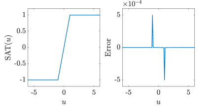
In Fig. 1, we present a comparison of the original saturation mapping and its approximation (10) for the value , in which a small approximation error is achieved.
In summary, we below present the design algorithm that we propose in this paper:
-
Step 1)
Let a reference set and initial gains , , , be given. Let and solve the optimization problem (7). Denote the solutions of the optimization problem as and . Set
and .
-
Step 2)
Set .
-
Step 3)
Generate initial states , …, randomly and uniformly from region .
-
Step 4)
Use ODE-Net to train the network under the loss function and find a set of controller parameters.
-
Step 5)
For , , , , and , Solve the optimization problem (7). Denote the solution as . If , let , , , , , and .
- Step 6)
-
Step 7)
, , , and are controller parameters and stop.
4 PERFORMANCE EVALUATION
In this section, we demonstrate the effectiveness of the proposed method based on numerical experiments. To demonstrate the effectiveness of our design method, let us consider the following open-loop unstable plant [7]:
The initial value of the dynamic controller is set to be
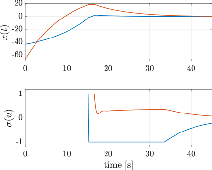
which is the same as the one used in [7]. Also, we let, , with and . Also, let , , , . Based on this setup, experiments were conducted in DiffEqFlux.jl [19] using Adam with a learning rate of and in DifferentialEquations.jl [20] using Runge-Kutta th order method for training. The optimization problem (7) is based on a reference set to find a larger ellipsoid centerd on the origin. Since the elements of the reference set exist only in the first quadrant, the initial value of step 3 of the design algorithm is randomly selected form the first and third quadrants of the region. The norm of the system when the initial value of the system is for the gains at is shown in the Fig. 2.
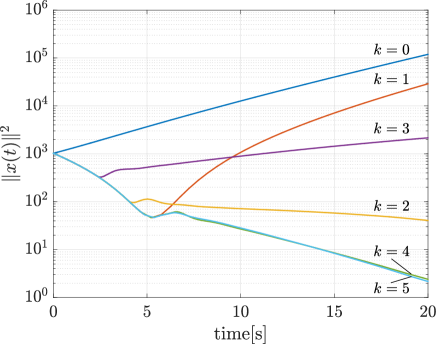
Fig. 2 shows that it is possible to find the gain that converges the state of the system to zero by applying the proposed method. is shown in Fig. 3.
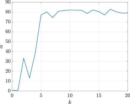
In Fig. 3, is increasing. Therefore, by solving problem 1 using an algorithm based on deep unfolding, we can find the gain to enlarge the ellipsoid. Also, is the largest when and , and each gain of the dynamic controller with anti-windup compensator was
In [7], when , the parameter indicating the size of the ellipsoid region is set to prevent high gain, , and without the constraint, . Using the itelative LMI [8], we obtained when , and we could not find a feasible solution in the absence of constraints. These values are obtained by solving a different optimization problem than optimization problem (7). However, the results in [8] and [7] are shown to be comparable [7]. The proposed method results in a larger ellipsoid region than the conventional method [7, 8]. The ellipsoid corresponding to the gain obtained by the proposed method and conventional method [8]. for is shown in Fig. 4. Fig. 4 shows that the system designed by the proposed method is more stable than the system designed by the conventional method [8] in a wide range.
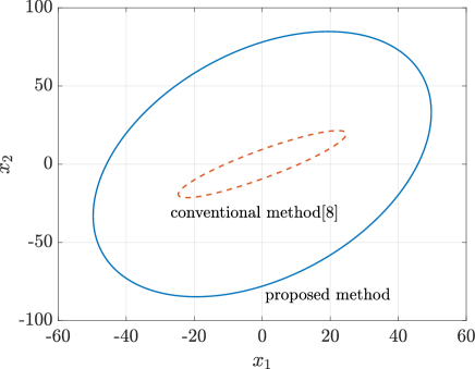
Fig. 5 shows a state response under the calculated gain. The initial condition is .
This initial condition is the value on the border of the ellipsoid. Fig. 5 shows that the values of the inputs are within the limits, and the state of the system is converged.
We verify that the proposed method is also valid for different reference sets. To show its validity, let the reference set be
We will compare the initial condition , which we give when designing, with the same case as in the example above, and the case where we choose from all the regions in region .
Let . When the initial condition was selected from the first and third quadrants as in the previous example, , and when the initial condition was selected from all regions, . If the value of the reference set is changed, a controller with a larger ellipsoid can be designed by changing the initial condition of the system given at the time of design. Applying [8], we obtain . In the case of changing the reference set, the ellipsoid of the proposed method became larger.
5 conclusion
In this note, we have proposed the deep unfolding-based design method of output feed controller for continuous-timesystems with input saturation. In the conventional method [7, 8], the dynamic controller is designed so that the closed-loop system becomes stable without considering input saturation, and the anti-windup controller is designed. On the other hand, proposed method design a dynamic controller and an anti-windup compensator considering input saturation.
In the numerical examples, we designed two reference sets to show the effectiveness of the proposed method. In the first numerical example, the controller designed with the proposed method has a larger absorption region than the conventional method [7, 8]. In the second numerical example, we changed the reference set. The proposed method enables us to enlarge the ellipsoid by changing the range of the initial state according to the reference set. Even when the reference set is changed, the ellipsoid is larger than that of the design by the conventional method.
References
- [1] T. Asakawa, I. Yamaguchi, Y. Hamada, T. Kasai, T. Nagashio, and T. Kida, “Anti-windup design for flexible spacecraft attitude control system”, in SICE Annual Conference 2011, pp. 1803–1806, 2011.
- [2] Y. Shinohara, K. Seki, M. Iwasaki, H. Chinda, and M. Takahashi, “Controller design for dual-stage actuator-driven load devices considering suppression of vibration due to input saturation”, in 2013 IEEE International Conference on Mechatronics, pp. 742–747, 2013.
- [3] K. Takaba, “Local synchronization of linear multi-agent systems subject to input saturation”, SICE Journal of Control, Measurement, and System Integration, Vol. 8, No. 5, pp. 334–340, 2015.
- [4] S. Tarbouriech and M. Turner, “Anti-windup design: an overview of some recent advances and open problems”, IET Control Theory & Applications, Vol. 3, No. 1, pp. 1–19, 2009.
- [5] V. R. Marcopoli and S. M. Phillips, “Analysis and synthesis tools for a class of actuator-limited multivariable control systems: A linear matrix inequality approach”, International Journal of Robust and Nonlinear Control, Vol. 6, No. 9-10, pp. 1045–1063, 1996.
- [6] E. F. Mulder, M. V. Kothare, and M. Morari, “Multivariable anti-windup controller synthesis using linear matrix inequalities”, Automatica, Vol. 37, No. 9, pp. 1407–1416, 2001.
- [7] J. M. G. da Silva and S. Tarbouriech, “Antiwindup design with guaranteed regions of stability: an LMI-based approach”, IEEE Transactions on Automatic Control, Vol. 50, No. 1, pp. 106–111, 2005.
- [8] Y. Y. Cao, Z. Lin, and D. G. Ward. “An antiwindup approach to enlarging domain of attraction for linear systems subject to actuator saturation”, IEEE Transactions on Automatic Control, Vol. 47, No. 1, pp. 140–145, 2002.
- [9] T. Kiyama and T. Iwasaki, “On the use of multi-loop circle criterion for saturating control synthesis”, Systems & Control Letters, Vol. 41, No. 2, pp. 105–114, 2000.
- [10] H. Ichihara and E. Nobuyama, “Stability analysis and control design of linear systems with input saturation using matrix sum of squares relaxation”, IFAC Proceedings Volumes, vol.39, no. 9, pp. 369–374, 2006.
- [11] T. Hu, Z. Lin, B. M. Chen, “An analysis and design method for linear systems subject to actuator saturation and disturbance”, Automatica, Vol. 38, No. 2, pp. 351–359, 2002,
- [12] J. M. G. Da Silva and S. Tarbouriech, “Local stabilization of discrete-time linear systems with saturating controls: an LMI-based approach”, IEEE Transactions on Automatic Control, Vol. 46, No. 1, pp. 119–125, 2001.
- [13] A. Balatsoukas and C. Studer, “Deep Unfolding for Communications Systems: A Survey and Some New Directions”, in 2019 IEEE International Workshop on Signal Processing Systems, pp. 266–271, 2019.
- [14] D. Ito, S. Takabe, and T. Wadayama, “Trainable ISTA for sparse signal recovery”, IEEE Transactions on Signal Processing, Vol. 67, No. 12, pp. 3113–3125, 2019.
- [15] M. Kishida, M. Ogura, Y. Yoshida, and T. Wadayama, “Deep learning-based average consensus”, IEEE Access, Vol. 8, pp. 142404–142412, 2020.
- [16] R. T. Q. Chen, Y. Rubanova, J. Bettencourt, and D. K Duvenaud, “Neural ordinary differential equations”, 32nd Conference on Neural Information Processing Systems, pp. 6571–6583, 2018.
- [17] A. R. Teel, “Anti-windup for exponentially unstable linear systems”, International Journal of Robust and Nonlinear Control, Vol. 9, No. 10, pp. 701–716, 1999.
- [18] O. Toker and H. Ozbay, “On the NP-hardness of solving bilinear matrix inequalities and simultaneous stabilization with static output feedback”, in 1995 American Control Conference, Vol. 4, pp. 2525–2526, 2005.
- [19] C. Rackauckas, M. Innes, Y. Ma,J. Bettencourt, L. White, and V. Dixit, “DiffEqFlux.jl - A julia library for neural differential equations”, arXiv:1902.02376, 2019.
- [20] C. Rackauckas and Q. Nie, “Differentialequations.jl – a performant and feature-rich ecosystem for solving differential equations in julia”, Journal of Open Research Software, Vol. 5, No. 1, p. 15, 2017.
- [21] P. Boscariol and A. Gasparetto, “Optimal trajectory planning for nonlinear systems: robust and constrained solution”, Robotica, Vol. 34, No. 6, pp. 1243-1259, 2016.