Deep Spectral Q-learning with Application to Mobile Health
Abstract
Dynamic treatment regimes assign personalized treatments to patients sequentially over time based on their baseline information and time-varying covariates. In mobile health applications, these covariates are typically collected at different frequencies over a long time horizon. In this paper, we propose a deep spectral Q-learning algorithm, which integrates principal component analysis (PCA) with deep Q-learning to handle the mixed frequency data. In theory, we prove that the mean return under the estimated optimal policy converges to that under the optimal one and establish its rate of convergence. The usefulness of our proposal is further illustrated via simulations and an application to a diabetes dataset.
Keywords: Dynamic Treatment Regimes, Mixed Frequency Data, Principal Component Analysis, Reinforcement Learning
1 Introduction
Precision medicine focuses on providing personalized treatment to patients by taking their personal information into consideration (see e.g., Kosorok and Laber, 2019; Tsiatis et al., 2019). It has found various applications in numerous studies, ranging from the cardiovascular disease study to cancer treatment and gene therapy (Jameson and Longo, 2015). A dynamic treatment regime (DTR) consists of a sequence of treatment decisions rules tailored to each individual patient’s status at each time, mathematically formulating the idea behind precision medicine. One of the major objectives in precision medicine is to identify the optimal dynamic treatment regime that yields the most favorable outcome on average.
With the rapidly development of mobile health (mHealth) technology, it becomes feasible to collect rich longitudinal data through mobile apps in medical studies. A motivating data example is given by the OhioT1DM dataset (Marling and Bunescu, 2020) which contains data from 12 patients suffering from type-I diabetes measured via fitness bands over 8 weeks. Data-driven decision rules estimated from these data have the potential to improve these patients’ health (see e.g., Shi et al., 2020; Zhu et al., 2020; Zhou et al., 2022). However, it remains challenging to estimate the optimal DTR in these mHealth studies. First, the number of treatment stages (e.g., horizon) is no longer fixed whereas the number of patients can be limited. For instance, in the OhioT1DM dataset, only 12 patients are enrolled in the study. Nonetheless, suppose treatment decisions are made on an hourly basis, the horizon is over 1000. Existing proposals in the DTR literature (Murphy, 2003; Zhang et al., 2013; Zhao et al., 2015; Song et al., 2015; Shi et al., 2018; Nie et al., 2021; Fang et al., 2022; Qi and Liu, 2018; Mo et al., 2021; Ertefaie et al., 2021; Guan et al., 2020; Zhang et al., 2018) become inefficient in these long or infinite horizon settings and require a large number of patients to be consistent. Second, patients’ time-varying covariates typically contain mixed frequency data. In the OhioT1DM dataset, some of the variables, such as the continuous glucose monitoring (CGM) blood glucose levels, are recorded every 5 minutes. Meanwhile, other variables, such as the carbohydrate estimate for the meal and the exercise intensity are recorded with a much lower frequency. Concatenating these high-frequency variables over each one-hour interval produces a high-dimensional state vector and directly using these states as input of the treatment policy would yield very noisy decision rules. A naive approach is to use some ad-hoc summaries of the high-frequency data for policy learning. However, this might produce a sub-optimal policy due to the information loss.
Recently, there is a growing line of research in the statistics literature for policy learning and/or evaluation in infinite horizons. Some references include Ertefaie and Strawderman (2018); Luckett et al. (2020); Shi et al. (2022); Liao et al. (2020, 2021); Shi et al. (2021c); Chen et al. (2022); Ramprasad et al. (2022); Li et al. (2022); Xu et al. (2020). In the computer science literature, there is a huge literature on developing reinforcement learning (RL) algorithms in infinite horizons. These algorithms can be casted into as model-free and model-based algorithms. Popular model-free RL methods include value-based methods that model the expected return starting from a given state (or state-action pair) and compute the optimal policy as the greedy policy with respect to the value function (Ernst et al., 2005; Riedmiller, 2005; Mnih et al., 2015; Van Hasselt et al., 2016; Dabney et al., 2018), and policy-based methods that directly search the optimal policy among a parameterized class via policy gradient or action critic methods (Schulman et al., 2015a, b; Koutník et al., 2013; Mnih et al., 2016; Wang et al., 2017b). Model-based algorithms are different from the model-free algorithms in the sense that they model the transition dynamics of the environment and use the model of environment to derive or improve policies. Popular model-based RL methods include Guestrin et al. (2002); Janner et al. (2019); Lai et al. (2020); Li et al. (2020), to name a few. See also Arulkumaran et al. (2017); Sutton and Barto (2018); Luo et al. (2022) for more details. These methods cannot be directly applied to datasets such as OhioT1DM as they haven’t considered the mixed frequency data.
In the RL literature, a few works have considered dimension reduction to handle the high dimensional state system. In particular, Murao and Kitamura (1997) proposed to segment the state space and learn a cluster representation of the states. Whiteson et al. (2007) proposed to divide the state space into tilings to represent each state. Both papers proposed to discretize the state space for dimension reduction. However, it can lead to considerable information loss (Wang et al., 2017a). Sprague (2007) proposed a iterative dimension reduction method using neighborhood components analysis. Their method uses a linear basis function to model the Q-function and cannot allow more general nonlinear function approximation. Recently, there are a few works that employ principal components analysis (PCA) for dimension reduction in RL (Curran et al., 2015, 2016; Parisi et al., 2017). However, none of the aforementioned papers formally established the theoretical guarantees for their proposals. Moreover, these methods are motivated by applications in games or robotics and their generalization to mHealth applications with mixed frequency data remains unknown.
In the DTR literature, a few works considered mixed frequency data which include both scalar and functional covariates. Specifically, McKeague and Qian (2014) proposed a functional regression model for optimal decision making with one functional covariate. Ciarleglio et al. (2015) and Ciarleglio et al. (2016) extended their proposal to a more general setting with multiple scalar and functional covariates. Ciarleglio et al. (2018) considered variable selection to handle the mixed frequency data. Laber and Staicu (2018) applied functional PCA to the functional covariates for dimension reduction. All these works considered single stage decision making. Their methods are not directly applicable to the infinite horizon settings.
Our contributions are as follows. Scientifically, mixed frequency data frequently arise in mHealth applications. Nonetheless, it has been less explored in the infinite horizon settings. Our proposal thus fills a crucial gap, and greatly extends the scope of existing approaches to learning DTRs. Methodologically, we propose a deep spectral Q-learning algorithm for dimension reduction. The proposed algorithm achieves a better empirical performance than those that either directly use the original mixed frequency data or its ad-hoc summaries as input of the treatment policy. Theoretically, we derive an upper error bound for the regret of the proposed policy and decompose this bound into the sum of approximation error and estimation error. Our theories offer some general guidelines for practitioners to select the number of principal components in the proposed algorithm.
The rest of this paper is organized as follows. We introduce some background about DTR and the mixed frequency data in Section 2. We introduce the proposed method to estimate the optimal DTR in Section 3 and study its theoretical properties in Section 4. Empirical studies are conducted in Section 5. In Section 5.3, we apply the proposed method to the OhioT1DM dataset. Finally, we conclude our paper in Section 6.
2 Preliminary
2.1 Data and Notations
Suppose the study enrolls patients. The dataset for the -th patient can be summarized as . For simplicity, we assume for any . Each state is composed of a set of low frequency covariates and a set of high frequency covariates , where is the state space. For each high frequency variable , we have for some large integer . Let denote the length of a time unit. The low frequency variables are recorded at time points . The th high frequency variables, however, are recorded more frequently at time points . Notice that we allow the high-frequency variables to be recorded with different frequencies. Let and denote a high-dimensional variable that concatenates all the high frequency covariates. As such, the state can be represented as . In addition, denotes the treatment indicator at the th time point and denotes the set of all possible treatment options. The reward, corresponds to the th patient’s response obtained after the th decision point. By convention, we assume a larger value of indicates a better outcome. We require to be uniformly bounded by some constant , and assume are , which are commonly imposed in the RL literature (see e.g., Sutton and Barto, 2018). Finally, we denote the -norm of a function aggregated over a given distribution function by . We use to represent the indices set for any integer .
2.2 Assumptions, Policies and Value Functions
We will require the system to satisfy the Markov assumption such that
for any and Borel set . In other words, the distribution of the next state depends on the past data history only through the current state-action pair. We assume the transition kernel is absolutely continuous with respect to some uniformly bounded transition density function such that for some constant .
In addition, we also impose the following conditional mean independence assumption:
where we refer to as the immediate reward function.
Next, define a policy as a function that maps a patient’s state at each time point into a probability distribution function on the action space. Given , we define its (state) value function as
with being a discount factor that balances the immediate and long-term rewards. By definition, the state value function characterizes the expected return assuming the decision process follows a given target policy . In addition, we define the state-action value function (or Q-function) as
which is the expected discounted cumulative rewards given an initial state-action pair.
Under the Markov assumption and the conditional mean independence assumption, there exists an optimal policy such that (see e.g., Puterman, 2014). Moreover, satisfies the following Bellman optimality equation:
| (1) |
where denotes the optimal Q-function.
2.3 ReLU Network
In this paper, we use value-based methods that learn the optimal policy by estimating the optimal Q-function. We will use the class of sparse neural network with the Rectified Linear Unit (ReLU) activation function, i.e., , to model the Q-function. The advantage of using a neural network over a simple parametric model is that the neural network can better capture the potential non-linearity in the high-dimensional state system.
Formally, the class of sparse ReLU network is defined as
Here, is the number of hidden layers of the neural network and is the width of each layer. The output dimension is set to 1 since the Q-function output is a scalar. The parameters in are the weight matrices and bias vectors . The sparsity level upper bounds the total number of nonzero parameters in the model. This constraint can be satisfied using dropout layers in the implementation (Srivastava et al., 2014). In theory, sparse ReLU networks can fit smooth functions with a minimax optimal rate of convergence (Schmidt-Hieber, 2020). The main theorems in Section 4 will rely on this property. An illustration of sparse ReLU network is in Figure 1.
3 Spectral Fitted Q-Iteration
Neural network with ReLU activation functions in 2.3 is commonly used in value-based reinforcement learning algorithms. However, in medical studies, the training dataset is often of limited size, with a few thousands or 10 thousands of observations in total (see e.g., Marling and Bunescu, 2020; Liao et al., 2021). Meanwhile, the data contains high frequency state variables, which yields a high-dimensional state system. Directly using these states as input will procedure a very noisy policy. This motivates us to consider dimension reduction in RL.
A naive approach for dimension reduction is to use some summary statistics of the high frequency state as input for policy learning. For instance, on the OhioT1DM dataset, the average of CGM blood glucose levels between two treatment decision points can be used as the summary statistic, as in Zhu et al. (2020); Shi et al. (2022); Zhou et al. (2022). In this paper, we propose to use principal component analysis to reduce the dimensionality of . We expect that using PCA can preserve more information than some ad-hoc summaries (e.g., average).
To apply PCA in the infinite horizon setting, we need to impose some stationarity assumptions on the concatenated high dimensional variables : and for some mean vector and covariance matrix that are independent of . In real data application, we can test whether the concatenated high-frequency variable is weak stationary (see e.g., Dickey and Fuller, 1979; Said and Dickey, 1984; Kwiatkowski et al., 1992). If it is weak stationary, the concatenated high frequency covariate will automatically satisfy the two assumptions above. Similar assumptions have been widely imposed in the literature (see e.g., Shi et al., 2021b; Kallus and Uehara, 2022). Without loss of generality, we assume for simplicity of notations. For the covariance matrix , it is generally unknown. In practice, we recommend to use the sample covariance estimator .
We describe our procedure as follows. By the spectral decomposition, we have , where are the eigenvalues and ’s are the corresponding eigenvectors. This allows us to represent as , where s are the estimated principal component scores, given by . For any , the estimated principal component scores correspond to the largest eigenvalues of the concatenated high frequency variable . When , using these principal component scores is equivalent to using the original high-frequency variable . We will approximate by and propose to use neural fitted Q-iteration algorithm by Riedmiller (2005) to learn the estimated optimal policy. We detail our procedure in Algorithm 1.
In Algorithm 1, we fit neural networks corresponding to each in . This is reasonable in settings where the action space is small. When the dataset is small (such as the OhioT1DM dataset), we recommend to set to such that all the data transactions (instead of a random subsample) will be used in each iteration.
Similar to the original neural fitted Q-iteration algorithm in Riedmiller (2005), the intuition of this algorithm is also based on the Bellman optimality equation (1). In each step of Algorithm 1, estimates and response corresponds to the right hand side of equation (1). Therefore, fitting the regression of with is to solve the Bellman optimality equation. The key difference between Algorithm 1 and original neural fitted Q-iteration algorithm is that the high dimensional inputs is involved in the state space, and is mapped to a lower dimensional vector during the learning process, so the neural networks takes principle components rather than original high dimensional as input.
4 Asymptotic Properties
Before discussing the asymptotic properties of our proposed Q-learning method, we introduce some notations.
Definition 4.1.
Define
where is the class of sparse ReLU network with layers and sparsity parameter and , the uniform upper bound for the cumulative reward.
We define as the Lipschitz constant for the sparse ReLU class used in . Note that this class is used in the original neural fitted Q-iteration algorithm to model the Q-function, where the dimension of high frequency part in state is not reduced through PCA. We further define a function class such that it models the Q-function by first converting high frequency part into its principal component scores and then use a sparse ReLU neural network to obtain the resulting Q-function. More specifically, is a set of functions , such that , where and is the vector containing first principle components of . Note that is the function class that we use in Algorithm 1 to model the Q-function. That is, (formal definition of and another function class not mentioned here are in Section A of Appendix).
In addition, we introduce the Hölder smooth function class by with to be the set of function input. The definition is:
Definition 4.2.
Define
where is a -tuple multi-index for partial derivatives.
We next construct a network structure with the component function on each layer of this network belonging to Holder smooth function class , which is called composition of Holder Smooth functions. This composition network contains layers, with each layer being , such that the th component () in layer satisfies that with inputs. Similar to the definition of , we can define the function class (simply denoted as ) on such that each function satisfies that for . The relation between function class and the network structure is similar to the relation between function class and the neural network in Definition 4.1. See Definition 4.1 of Fan et al. (2020) for more details on .
Next we will introduce the three major assumptions for our theorems:
Assumption 4.3.
The eigenvalues of follow an exponential decaying trend for some constant .
Assumption 4.4.
The estimator satisfies that for such that is some constant.
Assumption 4.5.
First, we define the Bellman optimality operator as
Then we assume for .
Among the three assumptions, the exponential decaying structure of eigenvalues in Assumption 4.3 can be commonly found in the literature of high-dimensional and functional data analysis (see e.g., Reiß and Wahl, 2020; Crambes and Mas, 2013; Jirak, 2016). This assumption is to control the information loss caused by using the first principal component scores of only. Assumption 4.4 is about the consistency of the estimators and similar assumptions are imposed in the literature of functional data analysis (see e.g., Laber and Staicu, 2018; Staicu et al., 2014). Using similar arguments in proving Theorem 5.2 of Zhang and Wang (2016), we can show that such an assumption holds in our setting as well. It is to bound the error caused by the estimation of the covariance matrix. Assumption 4.5 is referred to as the completeness assumption in the literature (see e.g., Chen and Jiang, 2019; Uehara et al., 2022, 2021). This assumption is automatically satisfied when the transition kernel and the reward function satisfy certain smoothness conditions.
Our first theorem is concerend with the nonasymptotic convergence rate of in Algorithm 1.
Theorem 4.6 (Convergence of Estimated Q-Function).
Let be some distribution on such that bounded away from . Under the Assumptions 4.3 to 4.5, with sufficiently large , there exists a sparse ReLU network structure for the function class modeling , such that obtained from our Algorithm 1 satisfies that:
where are some constants, is number of treatment options, and is the width of the first layer of the sparse ReLU network used in satisfying the bound .
More details of neural network structure and sample size assumptions for Theorem 4.6 can be found in Section B of Appendix. Theorem 4.6 provides an error bound on the estimated Q-function . Based on this theorem, we further establish the regret bound of the estimated policy obtained via Algorithm 1. Toward that end, we need another assumption:
Assumption 4.7.
Assume there exist , such that
for .
The margin type condition Assumption 4.7 is commonly used in the literature. Specifically, in classification, the margin conditions are imposed to bound the excess risk (Tsybakov, 2004; Audibert and Tsybakov, 2007). In dynamic treatment regime, a similar assumption is introduced for proving the convergence of State-Value function in a finite horizon setting (Qian and Murphy, 2011; Luedtke and van der Laan, 2016). In RL, these assumptions were introduced by (Shi et al., 2022) to obtain sharper regret bound for the estimated optimal policy.
Theorem 4.8 (Convergence of State-Value Function).
The proofs of the two theorems are included in Section C of Appendix. We summarize our theoretical findings below. First, we notice that the convergence rate of regret in Theorem 4.8 is faster than the convergence of estimated Q-functions in Theorem 4.6. This is due to the margin type Assumption 4.7 which enables us to obtain a sharper error bound. Similar results have been established in the literature. See e.g., Theorem 3.3 in Audibert and Tsybakov (2007), Theorem 3.1 in Qian and Murphy (2011), Theorems 3 and 4 in Shi et al. (2022).
From Theorem 4.8, it can be seen that the regret bound is mainly determined by three parameters: the sample size , the number of principal components and the number of iterations . Here, the first term on the right-hand-side corresponds to the estimation error, which decreases with and increases with . The second term corresponds to the approximation error, which decreases with both and . The remaining term is the optimization error which will decrease as the iteration number in Algorithm 1 grows.
Compared with the existing results on the convergence rate of deep fitted Q-iteration algorithm (see Theorem 4.4 of Fan et al., 2020), our theorems additionally characterize the dependence upon the number of principal components. Specifically, selecting the first principal components induces the information loss (e.g., bias) that is of the order , but reduces the model complexity caused by high frequency variables from to and hence the variance of the policy estimator. This represents a bias-variance trade-off. Notice that the bias decays at an exponential order, when the training data is small, reducing the model complexity can be more beneficial. Thus, our algorithm is expected to perform better than the original fitted Q-iteration algorithm in small samples, as shown in our numerical studies.
Finally, The number of principal components shall diverge with to ensure the consistency of the proposed algorithm. Based on the two theorems, the optimal that balances the bias and variance trade-off shall satisfy (details are given in Section D of Appendix). Thus, when goes to infinity, we will eventually take and our Algorithm 1 will be equivalent to the original neural fitted Q-iteration. This is just an asymptotic guideline for selecting the number of principal components. We provide some practical guidelines in the next section.
5 Empirical Studies
5.1 Practical Guidelines for Number of Principal Components
In functional data analysis, several criteria have been developed to select number of principal components, including the percentage of variance explained, Akaike information criterion (AIC) and Bayesian information criterion (BIC) (see e.g., Yao et al., 2005; Li et al., 2013). In our setting, it is difficult to apply AIC/BIC, since there does not exist a natural objective function (e.g., likelihood) for Q-function estimation. One possibility is to extend the value information criterion (Shi et al., 2021a) developed in single-stage decision making to infinite horizons. Nonetheless, it remains unclear how to determine the penalty parameter for consistent tuning parameter selection.
Here, we select based on the percentage of variance explained. That is, we can look at the minimum value of such that the total variance explained by PCA reaches a certain level (e.g., ). This method is also employed in Laber and Staicu (2018) in single-stage decision making. To illustrate the empirical performance of this method, we apply Algorithm 1 with and evaluate the expected return of these policies in the following numerical study.
The data generating process can be described as follows. We set the low frequency covariate to be a -dimensional vector and the high frequency variables to be a -dimensional vector (). Both are sampled from mean zero normal distributions. The covariance matrix of is set to satisfies Assumption 4.3. The action space is binary and the behavior policy to generate actions in training data is a uniform random policy. The reward function is set to for some constant and coefficient vectors such that it is a mixture of a linear function and a neural network with a single layer and ReLU activation function. Next state will be generated from a normal distribution with mean being a linear function of state and action . The number of trajectories is fixed to and the length of trajectory is set to be .
The ReLU network is constructed with 3 hidden layers and width . Dropout layers with dropout rate are added between layer 1, layer 2 and layer 3. During training, the dropout layers randomly sets the output from previous layers to with the probability , which can introduce sparsity to the neural network and reduce over-fitting (Srivastava et al., 2014). The hyperparamters of neural network structure can be tuned via cross-validation. The discounted factor is fixed to .
To evaluate the policy performance, we can use a Monte-Carlo method to approximate the expected return under each estimated policy. Specifically, for each estimated policy , we generate trajectories each of length (in our setting with , the cumulative reward after is negligible). The initial state distribution is the same as the one in the training dataset. The actions are assigned according to . The expected return can then be approximated via the average of the empirical cumulative rewards over the 100 trajectories.
For each in the list , we apply Algorithm 1 to learn the optimal policy over random seeds and evaluate their expected return using the Monte Carlo method. We then take the sample average and standard error of these expected returns to estimate the value of policy and construct the margin of error. Figure 2 depicts the estimated values of these expected returns as well as their confidence intervals. It can be seen that increasing from to leads to a significant improvement. However, further increasing worsens the performance. This trend is consistent with our theory since the bias term will dominate the estimation error for small value of . When increases, the bias decays at exponentially fast and the model complexity term becomes the leading term. Meanwhile, the percentage of variance explained increases quickly when and remains stable afterwards. As such, it makes sense to use this criterion for selection. In our implementation, we select the smallest such that the variance explained is at least .
5.2 Simulation Study
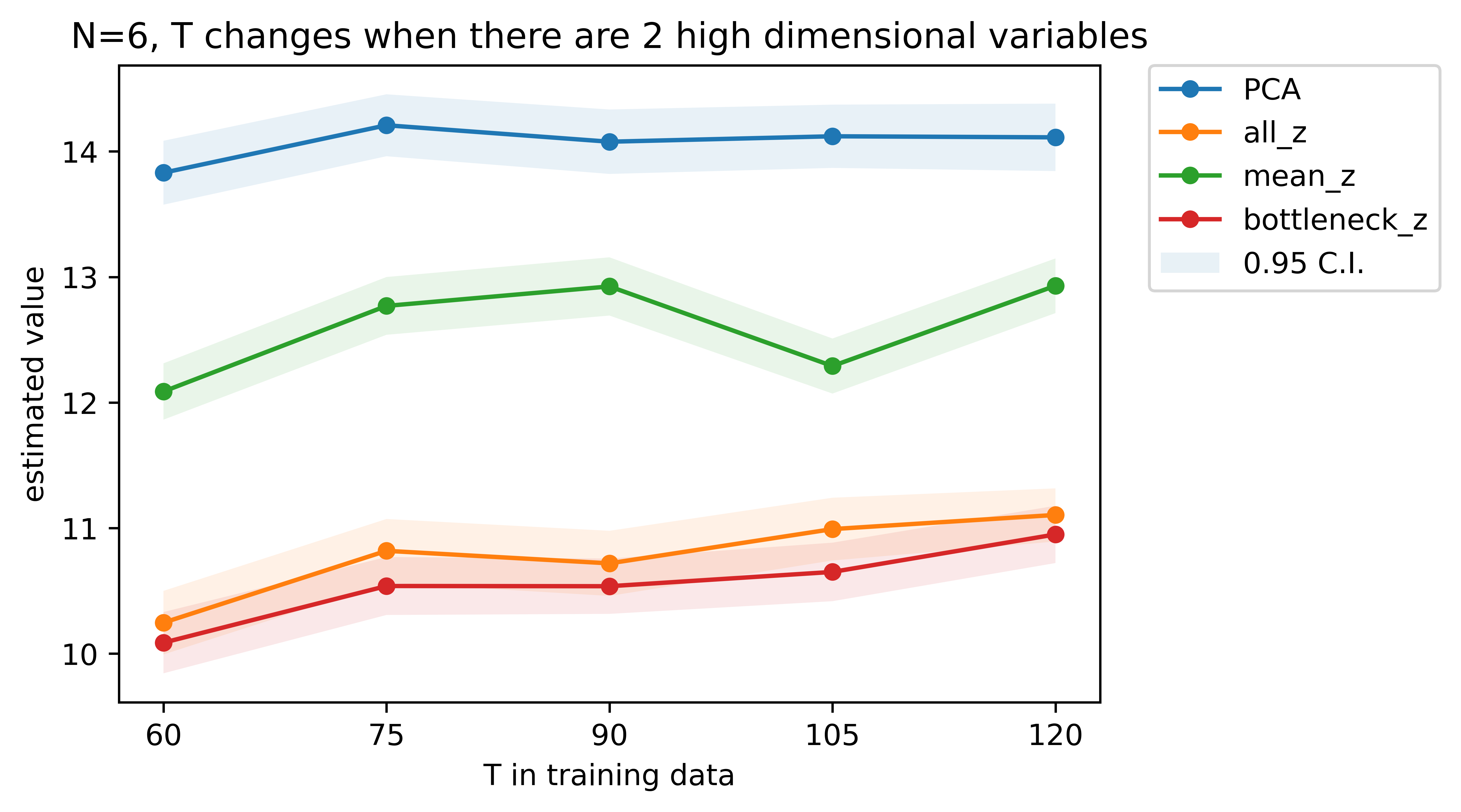
In the simulation study, we compare the proposed policy against two baseline policies obtained by directly using the original high frequency variable (denoted by ) and its average as input (denoted by ). Both policies are computed in a similar manner based on the deep fitted Q-iteration algorithm. We additionally include one more baseline policy, denoted by , which adds one bottleneck layer after the input of original in the neural network architecture such that the width of this bottleneck layer is the same as the input dimension of the proposed policy . This policy differs from the proposed policy in that it uses this bottleneck layer for dimension reduction instead of PCA. Both the data generating setting and the neural network structure are the same to Section 5.1. However, in this simulation study we vary the sample size and the dimension of the high frequency variables. Specifically, we consider 9 cases of training size ( and ) and different high frequency part dimension . Furthermore, we have two settings of generating high frequency variables that will be discussed below. We similarly compare the proposed policy against , , and and use the Monte Carlo method to evaluate their values.
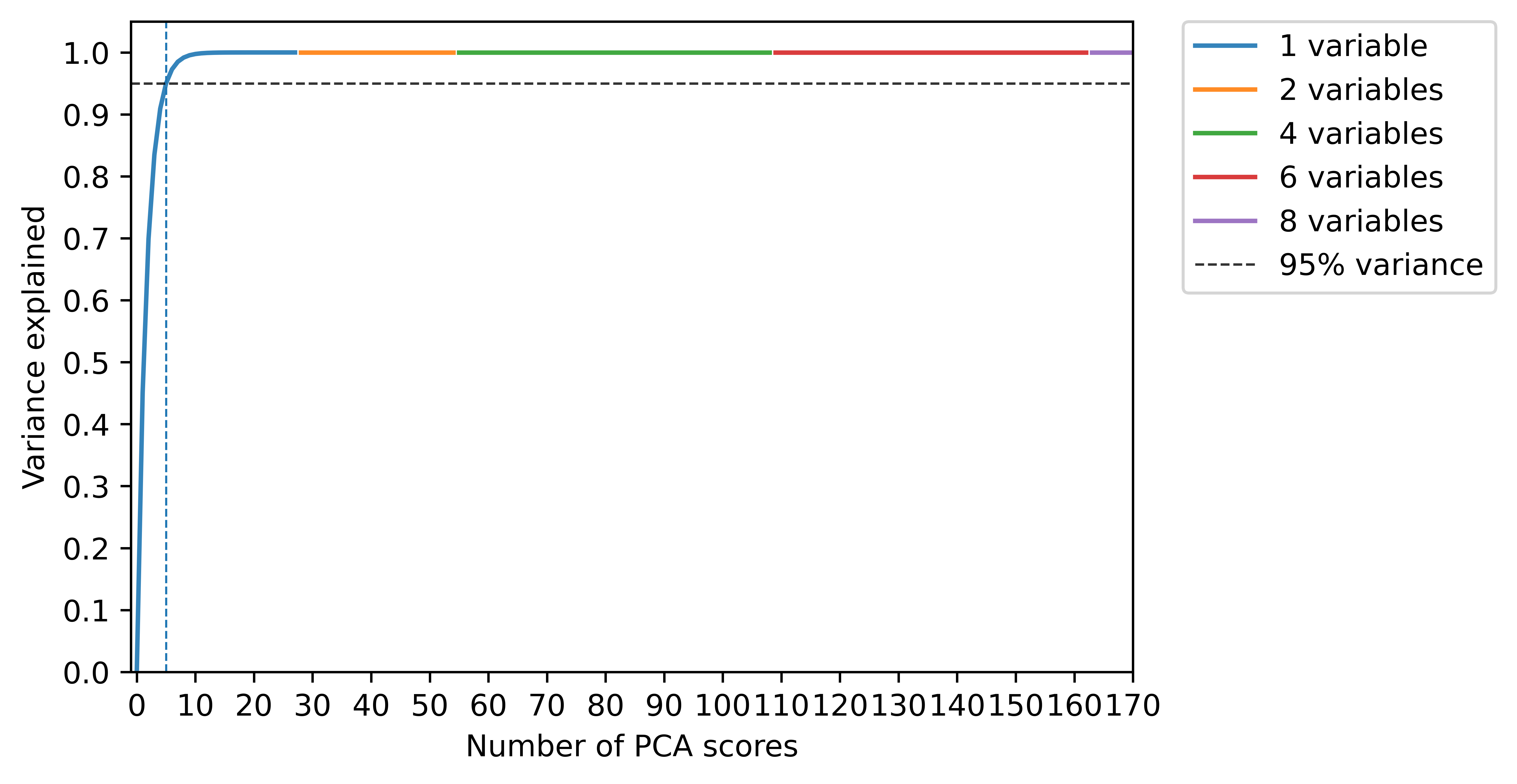
In the first setting, we consider cases with (the number of high frequency variables) equals and each high frequency variable is of dimension . In this setting, all high frequency variables are dependent and eigenvalues of concatenated high frequency variable decays at an exponential order. We find that the first principal components explains over of variance in all the cases, as shown in Figure 3. Therefore, we set the number of principal components and plot the results in Figure 4.
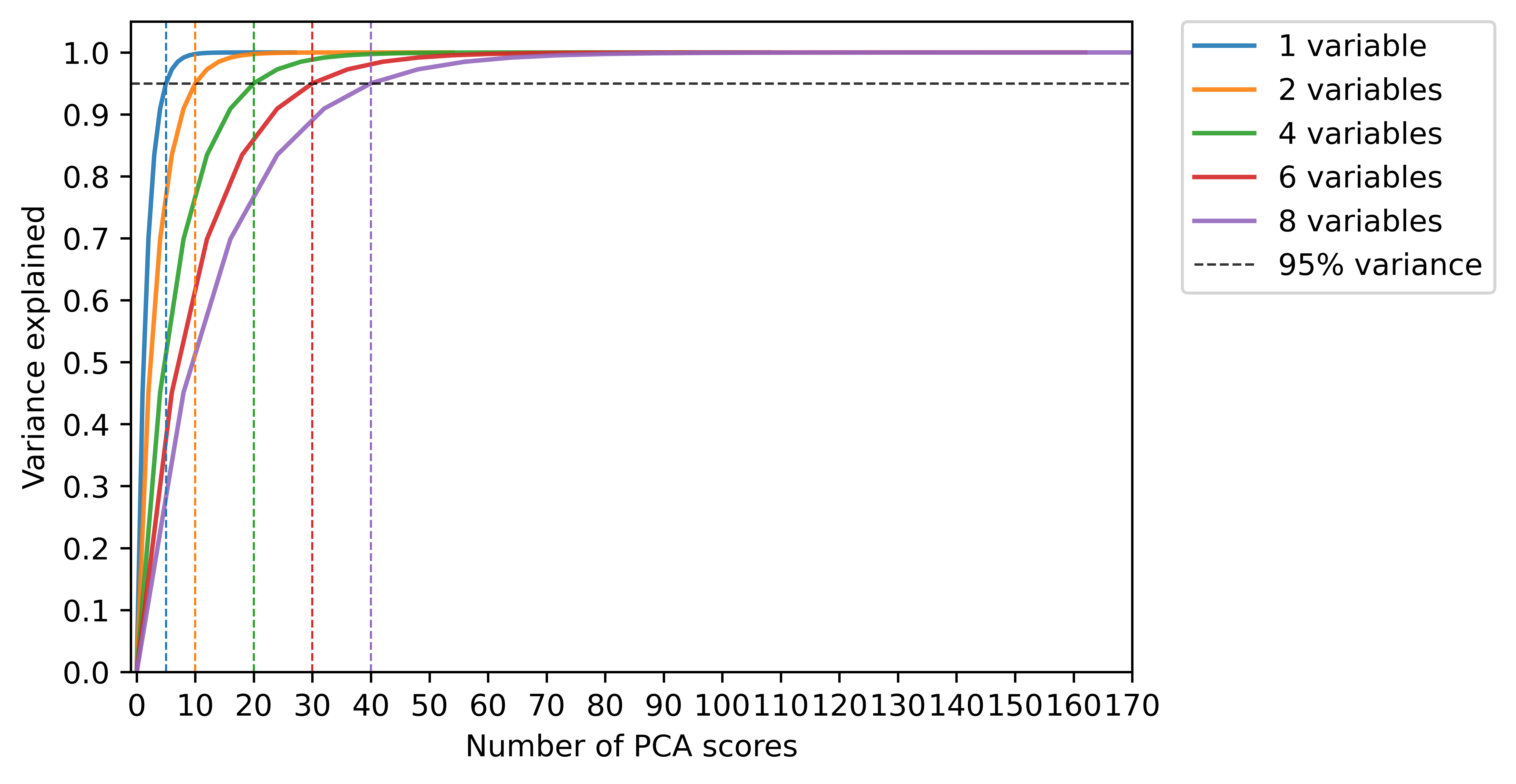
In the second setting, the high frequency variables are independent with each other. For each , all the elements in are dependent and eigenvalues of decays at the same exponential order as the eigenvalues of the concatenated high frequency variable in the first setting. Therefore, more principal components are needed to guarantee that the number of variance explained exceeds , as increases. Specifically, when high frequency variables, the corresponding is given by accordingly. See Figure 3 for details. The expected returns of all estimated optimal policies are plotted in Figure 5.
From Figures 4 and 5, it can be seen that the proposed policy always achieves a larger value than the three baseline policies. Meanwhile, and perform comparably. The value of both of them are significantly affected by the training size . In addition, outperforms and in small samples, but performs worse than the two policies when the sample size is large. In the second setting, and tend to perform much better than when , since averaging over several high frequency variables will lose more relevant information for policy learning.
Finally, we conduct an additional simulation study with large training datasets where or and . This setting might be unrealistic in an mHealth dataset. It is included only to test the performance of . As is consistent as well, we anticipate that the difference between the value under and the proposed policy will be negligible as the sample size grows to infinity. Figure 6 depicts the results. As expected, we observe no significant difference between and when .
5.3 Application on OhioT1DM Dataset
We apply the proposed Algorithm 1 on the updated OhioT1DM Dataset by Marling and Bunescu (2020). In the real data case, we would still like to compare the behaviors of the four policies: , , and . OhioT1DM Dataset contains medical information of 12 type-I diabetes patients, including the CGM blood glucose levels of the patients, insulin doses applied during this period, self-reported information of meals and exercises, and other variables recorded by mobile phone apps and physiological sensors. The high frequency variables in the OhioT1DM Dataset, such as CGM blood glucose levels, are recorded every 5 minutes. The data for exercises and meals are collected with a much lower frequency, say recorded every few hours. Moreover, considering the basal insulin rate of in this dataset, although this variable is also collected every minutes, it usually remains a constant for several hours in a day. Thus, the basal insulin rate can also be regarded as a low-frequency scalar variable by taking the average of it. The time period between two decision points is set as hours, as we only consider non-emergency situations where patients don’t need to take bolus injection promptly. In other studies using the OhioT1DM Dataset, the treatment decision frequency is also set to be much lower than the recording frequency of CGM blood glucose levels (see e.g., Shi et al., 2022; Zhou et al., 2021; Zhu et al., 2020).
For the low frequency covariate , is constructed based on the th patient’s self-reported carbohydrate estimate for the meal during the past -hour-interval . The second scalar variable in is defined as the average of the basal rate of insulin dose during the past interval . We consider one high-frequency element, , which contains CGM blood glucose levels recorded every 5 minutes during the past hours (its dimension is ). The action variable is set to when the total amount of insulin delivered to the -th patient is greater than one unit in the past interval. The response variable is defined according to the Index of Glycemic Control (IGC, Rodbard, 2009), which is a non-linear function of the blood glucose levels in the following stage. A higher IGC value indicates that the blood glucose level of this patient stays close or falls in to the proper range of glucose level.
In this study, is selected when training , as the proportion of variance explained by the first principal components is over , as is shown in Figure 7. The ReLU network here is with 2 hidden layers and width (dropout layers with dropout rate added between layer 1, layer 2 and the output layer). To estimate the value of the four policies, we use the Fitted Q Evaluation algorithm proposed by Le et al. (2019). When applying the Fitted Q Evaluation algorithm, a random forest model is used to fit the estimated Q-function of the policy to be evaluated. By dividing patients into a training set of patients and testing set of patients, there are repetitions with different patient combinations. In each repetition, the data of patients is used to train the policy and fit the random forest for Fitted Q Evaluation corresponding to this policy. The data of the other patient is used for approximating the value of the policy using the estimated Q-function from Fitted Q Evaluation. The sample mean of estimated values from all repetitions is taken as our main result and the standard errors are used to construct the margin of error. To compare the performance of our proposed policies against , , and , we present the difference of estimated values of and the three other policies in Table 1, where margin of error is standard error of the mean difference multiplied by the critical value . The estimated values of the four policies is in Table 2.
Based on the result, it can be shown that the estimated value of is higher than all three baselines. The policy obtained by using the average of CGM blood glucose levels is commonly used in literature (Zhou et al., 2021; Zhu et al., 2020). The less plausible performance of is probably due to the information loss by simply replacing the CGM blood glucose levels with its average. On the other hand, the size of training data is relatively small, as we didn’t use all the data recorded in eight weeks due to the large chunks of missing values. Eventually training data from about 5 consecutive weeks are used for training DTR policies. In such scenarios, using the original high frequency vector will significantly increase the complexity of the ReLU network structure, such that the number of parameters to be trained is too large compared to the size of training data. Thus, and cannot outperform where input dimension is reduced by PCA. The results shown in Table 1 and Table 2 agree with the results in Section 5.2.
6 Discussions
In summary, we propose a deep spectral fitted Q-iteration algorithm to handle mixed frequency data in infinite horizon settings. The algorithm relies on the use of PCA for dimension reduction and the use of deep neural networks to capture the non-linearity in the high-dimensional system. In theory, we establish a regret bound for the estimated optimal policy. Our theorem provides an asymptotic guideline for selecting the number of principal components. In empirical studies, we demonstrate the superiority of the proposed algorithm over baseline methods without dimension reduction or use ad-hoc summaries of the state. We further offer practical guidelines to select the number of principal components. The proposed paper is built upon on PCA and deep Q-learning. It is worthwhile to investigate the performance of other dimension reduction and RL methods. We leave it for future research.
References
- Arulkumaran et al. (2017) Arulkumaran, K., Deisenroth, M. P., Brundage, M., and Bharath, A. A. “Deep reinforcement learning: A brief survey.” IEEE Signal Processing Magazine, 34(6):26–38 (2017).
- Audibert and Tsybakov (2007) Audibert, J. and Tsybakov, A. “Fast learning rates for plug-in classifiers.” The Annals of statistics, 35(2):608–633 (2007).
- Chen et al. (2022) Chen, E. Y., Song, R., and Jordan, M. I. “Reinforcement Learning with Heterogeneous Data: Estimation and Inference.” arXiv preprint arXiv:2202.00088 (2022).
- Chen and Jiang (2019) Chen, J. and Jiang, N. “Information-theoretic considerations in batch reinforcement learning.” International Conference on Machine Learning, 1042–1051 (2019).
- Ciarleglio et al. (2015) Ciarleglio, A., Petkova, E., Ogden, R. T., and Tarpey, T. “Treatment decisions based on scalar and functional baseline covariates.” Biometrics, 71(4):884–894 (2015).
- Ciarleglio et al. (2018) Ciarleglio, A., Petkova, E., Ogden, T., and Tarpey, T. “Constructing treatment decision rules based on scalar and functional predictors when moderators of treatment effect are unknown.” Journal of the Royal Statistical Society. Series C, Applied statistics, 67(5):1331 (2018).
- Ciarleglio et al. (2016) Ciarleglio, A., Petkova, E., Tarpey, T., and Ogden, R. T. “Flexible functional regression methods for estimating individualized treatment rules.” Stat (Int Stat Inst), 5(1):185–199 (2016).
- Crambes and Mas (2013) Crambes, C. and Mas, A. “Asymptotics of prediction in functional linear regression with functional outputs.” Bernoulli, 2627–2651 (2013).
- Curran et al. (2016) Curran, W., Brys, T., Aha, D., Taylor, M., and Smart, W. D. “Dimensionality reduced reinforcement learning for assistive robots.” In 2016 AAAI Fall Symposium Series (2016).
- Curran et al. (2015) Curran, W., Brys, T., Taylor, M., and Smart, W. “Using PCA to efficiently represent state spaces.” arXiv preprint arXiv:1505.00322 (2015).
- Dabney et al. (2018) Dabney, W., Rowland, M., Bellemare, M., and Munos, R. “Distributional reinforcement learning with quantile regression.” Thirty-Second AAAI Conference on Artificial Intelligence (2018).
- Dickey and Fuller (1979) Dickey, D. A. and Fuller, W. A. “Distribution of the estimators for autoregressive time series with a unit root.” Journal of the American statistical association, 74(366a):427–431 (1979).
- Ernst et al. (2005) Ernst, D., Geurts, P., and Wehenkel, L. “Tree-based batch mode reinforcement learning.” Journal of Machine Learning Research, 6:503–556 (2005).
- Ertefaie et al. (2021) Ertefaie, A., McKay, J. R., Oslin, D., and Strawderman, R. L. “Robust Q-learning.” Journal of the American Statistical Association, 116(533):368–381 (2021).
- Ertefaie and Strawderman (2018) Ertefaie, A. and Strawderman, R. L. “Constructing dynamic treatment regimes over indefinite time horizons.” Biometrika, 105(4):963–977 (2018).
- Fan et al. (2020) Fan, J., Wang, Z., Xie, Y., and Yang, Z. “A theoretical analysis of deep Q-learning.” Learning for Dynamics and Control, 486–489 (2020).
- Fang et al. (2022) Fang, E. X., Wang, Z., and Wang, L. “Fairness-Oriented Learning for Optimal Individualized Treatment Rules.” Journal of the American Statistical Association, 1–14 (2022).
- Guan et al. (2020) Guan, Q., Reich, B. J., Laber, E. B., and Bandyopadhyay, D. “Bayesian nonparametric policy search with application to periodontal recall intervals.” Journal of the American Statistical Association, 115(531):1066–1078 (2020).
- Guestrin et al. (2002) Guestrin, C., Patrascu, R., and Schuurmans, D. “Algorithm-directed exploration for model-based reinforcement learning in factored MDPs.” In ICML, 235–242. Citeseer (2002).
- Jameson and Longo (2015) Jameson, J. L. and Longo, D. L. “Precision medicine—personalized, problematic, and promising.” Obstetrical & gynecological survey, 70(10):612–614 (2015).
- Janner et al. (2019) Janner, M., Fu, J., Zhang, M., and Levine, S. “When to trust your model: Model-based policy optimization.” Advances in Neural Information Processing Systems, 32 (2019).
- Jirak (2016) Jirak, M. “Optimal eigen expansions and uniform bounds.” Probability Theory and Related Fields, 166(3):753–799 (2016).
- Kallus and Uehara (2022) Kallus, N. and Uehara, M. “Efficiently breaking the curse of horizon in off-policy evaluation with double reinforcement learning.” Operations Research (2022).
- Kosorok and Laber (2019) Kosorok, M. R. and Laber, E. B. “Precision medicine.” Annual review of statistics and its application, 6:263–286 (2019).
- Koutník et al. (2013) Koutník, J., Cuccu, G., Schmidhuber, J., and Gomez, F. “Evolving large-scale neural networks for vision-based reinforcement learning.” Proceedings of the 15th annual conference on Genetic and evolutionary computation, 1061–1068 (2013).
- Kwiatkowski et al. (1992) Kwiatkowski, D., Phillips, P. C., Schmidt, P., and Shin, Y. “Testing the null hypothesis of stationarity against the alternative of a unit root: How sure are we that economic time series have a unit root?” Journal of econometrics, 54(1-3):159–178 (1992).
- Laber and Staicu (2018) Laber, E. and Staicu, A. “Functional feature construction for individualized treatment regimes.” Journal of the American Statistical Association, 113(523):1219–1227 (2018).
- Lai et al. (2020) Lai, H., Shen, J., Zhang, W., and Yu, Y. “Bidirectional model-based policy optimization.” In International Conference on Machine Learning, 5618–5627. PMLR (2020).
- Lazaric et al. (2016) Lazaric, A., Ghavamzadeh, M., and Munos, R. “Analysis of classification-based policy iteration algorithms.” Journal of Machine Learning Research, 17:583–612 (2016).
- Le et al. (2019) Le, H., Voloshin, C., and Yue, Y. “Batch policy learning under constraints.” International Conference on Machine Learning, 3703–3712 (2019).
- Li et al. (2020) Li, G., Wei, Y., Chi, Y., Gu, Y., and Chen, Y. “Breaking the sample size barrier in model-based reinforcement learning with a generative model.” Advances in neural information processing systems, 33:12861–12872 (2020).
- Li et al. (2022) Li, Y., Wang, C.-h., Cheng, G., and Sun, W. W. “Rate-Optimal Contextual Online Matching Bandit.” arXiv preprint arXiv:2205.03699 (2022).
- Li et al. (2013) Li, Y., Wang, N., and Carroll, R. J. “Selecting the number of principal components in functional data.” Journal of the American Statistical Association, 108(504):1284–1294 (2013).
- Liao et al. (2021) Liao, P., Klasnja, P., and Murphy, S. “Off-policy estimation of long-term average outcomes with applications to mobile health.” Journal of the American Statistical Association, 116(533):382–391 (2021).
- Liao et al. (2020) Liao, P., Qi, Z., Klasnja, P., and Murphy, S. “Batch policy learning in average reward markov decision processes.” arXiv preprint arXiv:2007.11771 (2020).
-
Luckett et al. (2020)
Luckett, D. J., Laber, E. B., Kahkoska, A. R., Maahs, D. M., Mayer-Davis, E.,
and Kosorok, M. R.
“Estimating Dynamic Treatment Regimes in Mobile Health Using
V-Learning.”
Journal of the American Statistical Association,
115(530):692–706 (2020).
PMID: 32952236.
URL https://doi.org/10.1080/01621459.2018.1537919 -
Luedtke and van der Laan (2016)
Luedtke, A. R. and van der Laan, M. J.
“Statistical inference for the mean outcome under a possibly
non-unique optimal treatment strategy.”
The Annals of Statistics, 44(2):713 – 742 (2016).
URL https://doi.org/10.1214/15-AOS1384 - Luo et al. (2022) Luo, F.-M., Xu, T., Lai, H., Chen, X.-H., Zhang, W., and Yu, Y. “A survey on model-based reinforcement learning.” arXiv preprint arXiv:2206.09328 (2022).
- Marling and Bunescu (2020) Marling, C. and Bunescu, R. “The OhioT1DM Dataset for Blood Glucose Level Prediction: Update 2020.” CEUR workshop proceedings, 2675:71–74 (2020).
- McKeague and Qian (2014) McKeague, I. W. and Qian, M. “Estimation of treatment policies based on functional predictors.” Statistica Sinica, 24(3):1461 (2014).
- Mnih et al. (2016) Mnih, V., Badia, A., Mirza, M., Graves, A., Lillicrap, T., Harley, T., Silver, D., and Kavukcuoglu, K. “Asynchronous methods for deep reinforcement learning.” International conference on machine learning, 1928–1937 (2016).
- Mnih et al. (2015) Mnih, V., Kavukcuoglu, K., Silver, D., Rusu, A., Veness, J., Bellemare, M., Graves, R., A., M., F., A.K., G., Ostrovski, and Petersen, S. “Human-level control through deep reinforcement learning.” nature, 518(7540):529–533 (2015).
- Mo et al. (2021) Mo, W., Qi, Z., and Liu, Y. “Learning optimal distributionally robust individualized treatment rules.” Journal of the American Statistical Association, 116(534):659–674 (2021).
- Murao and Kitamura (1997) Murao, H. and Kitamura, S. “Q-learning with adaptive state segmentation (QLASS).” In Proceedings 1997 IEEE International Symposium on Computational Intelligence in Robotics and Automation CIRA’97.’Towards New Computational Principles for Robotics and Automation’, 179–184 (1997).
- Murphy (2003) Murphy, S. A. “Optimal dynamic treatment regimes.” Journal of the Royal Statistical Society: Series B (Statistical Methodology), 65(2):331–355 (2003).
- Nie et al. (2021) Nie, X., Brunskill, E., and Wager, S. “Learning when-to-treat policies.” Journal of the American Statistical Association, 116(533):392–409 (2021).
- Parisi et al. (2017) Parisi, S., Ramstedt, S., and Peters, J. “Goal-driven dimensionality reduction for reinforcement learning.” In 2017 IEEE/RSJ International Conference on Intelligent Robots and Systems (IROS), 4634–4639. IEEE (2017).
- Puterman (2014) Puterman, M. L. Markov decision processes: discrete stochastic dynamic programming. John Wiley & Sons (2014).
- Qi and Liu (2018) Qi, Z. and Liu, Y. “D-learning to estimate optimal individual treatment rules.” Electronic Journal of Statistics, 12(2):3601–3638 (2018).
- Qian and Murphy (2011) Qian, M. and Murphy, S. A. “Performance guarantees for individualized treatment rules.” Annals of statistics, 39(2):1180 (2011).
- Ramprasad et al. (2022) Ramprasad, P., Li, Y., Yang, Z., Wang, Z., Sun, W. W., and Cheng, G. “Online bootstrap inference for policy evaluation in reinforcement learning.” Journal of the American Statistical Association, 1–14 (2022).
- Reiß and Wahl (2020) Reiß, M. and Wahl, M. “Nonasymptotic upper bounds for the reconstruction error of PCA.” The Annals of Statistics, 48(2):1098–1123 (2020).
- Riedmiller (2005) Riedmiller, M. “Neural fitted Q iteration–first experiences with a data efficient neural reinforcement learning method.” European Conference on Machine Learning, 317–328 (2005).
- Rodbard (2009) Rodbard, D. “Interpretation of continuous glucose monitoring data: glycemic variability and quality of glycemic control.” Diabetes technology & therapeutics, 11(S1):S–55 (2009).
- Said and Dickey (1984) Said, S. E. and Dickey, D. A. “Testing for unit roots in autoregressive-moving average models of unknown order.” Biometrika, 71(3):599–607 (1984).
- Schmidt-Hieber (2020) Schmidt-Hieber, J. “Nonparametric regression using deep neural networks with ReLU activation function.” The Annals of Statistics, 48(4):1875–1897 (2020).
- Schulman et al. (2015a) Schulman, J., Levine, S., Abbeel, P., Jordan, M., and Moritz, P. “Trust region policy optimization.” International conference on machine learning, 1889–1897 (2015a).
- Schulman et al. (2015b) Schulman, J., Moritz, P., Levine, S., Jordan, M., and Abbeel, P. “High-dimensional continuous control using generalized advantage estimation.” arXiv preprint arXiv:1506.02438 (2015b).
- Shi et al. (2021a) Shi, C., Song, R., and Lu, W. “Concordance and value information criteria for optimal treatment decision.” The Annals of Statistics, 49(1):49–75 (2021a).
- Shi et al. (2018) Shi, C., Song, R., Lu, W., and Fu, B. “Maximin projection learning for optimal treatment decision with heterogeneous individualized treatment effects.” Journal of the Royal Statistical Society: Series B (Statistical Methodology), 80(4):681–702 (2018).
- Shi et al. (2021b) Shi, C., Wan, R., Chernozhukov, V., and Song, R. “Deeply-debiased off-policy interval estimation.” In International Conference on Machine Learning, 9580–9591. PMLR (2021b).
- Shi et al. (2020) Shi, C., Wan, R., Song, R., Lu, W., and Leng, L. “Does the Markov Decision Process Fit the Data: Testing for the Markov Property in Sequential Decision Making.” In International Conference on Machine Learning, 8807–8817. PMLR (2020).
- Shi et al. (2021c) Shi, C., Wang, X., Luo, S., Zhu, H., Ye, J., and Song, R. “Dynamic causal effects evaluation in A/B testing with a reinforcement learning framework.” Journal of the American Statistical Association, accepted (2021c).
- Shi et al. (2022) Shi, C., Zhang, S., Lu, W., and Song, R. “Statistical inference of the value function for reinforcement learning in infinite horizon settings.” Journal of the Royal Statistical Society: Series B, 84:765–793 (2022).
- Song et al. (2015) Song, R., Wang, W., Zeng, D., and Kosorok, M. R. “Penalized q-learning for dynamic treatment regimens.” Statistica Sinica, 25(3):901 (2015).
- Sprague (2007) Sprague, N. “Basis iteration for reward based dimensionality reduction.” 2007 IEEE 6th International Conference on Development and Learning, 187–192 (2007).
- Srivastava et al. (2014) Srivastava, N., Hinton, G., Krizhevsky, A., Sutskever, I., and Salakhutdinov, R. “Dropout: a simple way to prevent neural networks from overfitting.” The journal of machine learning research, 15(1):1929–1958 (2014).
- Staicu et al. (2014) Staicu, A.-M., Li, Y., Crainiceanu, C. M., and Ruppert, D. “Likelihood ratio tests for dependent data with applications to longitudinal and functional data analysis.” Scandinavian Journal of Statistics, 41(4):932–949 (2014).
- Sutton and Barto (2018) Sutton, R. S. and Barto, A. G. Reinforcement learning: an introduction. MIT Press (2018).
- Tsiatis et al. (2019) Tsiatis, A. A., Davidian, M., Holloway, S. T., and Laber, E. B. Dynamic treatment regimes: Statistical methods for precision medicine. Chapman and Hall/CRC (2019).
- Tsybakov (2004) Tsybakov, A. “Optimal aggregation of classifiers in statistical learning.” The Annals of Statistics, 32(1):135–166 (2004).
- Uehara et al. (2021) Uehara, M., Imaizumi, M., Jiang, N., Kallus, N., Sun, W., and Xie, T. “Finite sample analysis of minimax offline reinforcement learning: Completeness, fast rates and first-order efficiency.” arXiv preprint arXiv:2102.02981 (2021).
- Uehara et al. (2022) Uehara, M., Kiyohara, H., Bennett, A., Chernozhukov, V., Jiang, N., Kallus, N., Shi, C., and Sun, W. “Future-dependent value-based off-policy evaluation in pomdps.” arXiv preprint arXiv:2207.13081 (2022).
- Van Hasselt et al. (2016) Van Hasselt, H., Guez, A., and Silver, D. “Deep reinforcement learning with double q-learning.” Proceedings of the AAAI conference on artificial intelligence, 30(1) (2016).
- Wang et al. (2017a) Wang, L., Laber, E. B., and Witkiewitz, K. “Sufficient Markov decision processes with alternating deep neural networks.” arXiv preprint, arXiv:1704.07531 (2017a).
- Wang et al. (2017b) Wang, Z., Bapst, V., Heess, N., Mnih, V., Munos, R., Kavukcuoglu, K., and de Freitas, N. “Sample efficient actor-critic with experience replay.” ICLR (2017b).
- Whiteson et al. (2007) Whiteson, S., Taylor, M. E., and Stone, P. “Adaptive Tile Coding for Value Function Approximation.” (2007).
- Xu et al. (2020) Xu, Z., Laber, E., Staicu, A.-M., and Severus, E. “Latent-state models for precision medicine.” arXiv preprint arXiv:2005.13001 (2020).
- Yao et al. (2005) Yao, F., Müller, H.-G., and Wang, J.-L. “Functional data analysis for sparse longitudinal data.” Journal of the American statistical association, 100(470):577–590 (2005).
- Zhang et al. (2013) Zhang, B., Tsiatis, A. A., Laber, E. B., and Davidian, M. “Robust estimation of optimal dynamic treatment regimes for sequential treatment decisions.” Biometrika, 100(3):681–694 (2013).
- Zhang and Wang (2016) Zhang, X. and Wang, J. “From sparse to dense functional data and beyond.” The Annals of Statistics, 44(5):2281–2321 (2016).
- Zhang et al. (2018) Zhang, Y., Laber, E. B., Davidian, M., and Tsiatis, A. A. “Interpretable dynamic treatment regimes.” Journal of the American Statistical Association, 113(524):1541–1549 (2018).
- Zhao et al. (2015) Zhao, Y.-Q., Zeng, D., Laber, E. B., and Kosorok, M. R. “New statistical learning methods for estimating optimal dynamic treatment regimes.” Journal of the American Statistical Association, 110(510):583–598 (2015).
- Zhou et al. (2021) Zhou, W., Zhu, R., and Qu, A. “Estimating Optimal Infinite Horizon Dynamic Treatment Regimes via pT-Learning.” arXiv preprint arXiv:2110.10719 (2021).
- Zhou et al. (2022) —. “Estimating Optimal Infinite Horizon Dynamic Treatment Regimes via pT-Learning.” Journal of the American Statistical Association, accepted (2022).
- Zhu et al. (2020) Zhu, L., Lu, W., and Song, R. “Causal effect estimation and optimal dose suggestions in mobile health.” In International Conference on Machine Learning, 11588–11598. PMLR (2020).
Appendix A Supplementary Definitions
In this section we would like to introduce more definitions, which will be used in the rest of supporting information.
Note that is a function class to model the Q-function without using PCA. We need to define two more function classes based on PCA of the high dimensional input :
Definition A.1.
where is defined in Section 4 and is the covariance matrix of . is the vector recovered from the first PCA values of the original high-frequency vector .
The definition of is already mentioned in Section 4. Here we would like to formally define it as below:
where is the vector containing first PCA values of the original high-frequency vector .
Note that is the function class that we use in Spectrum Q-Iterated Learning Algorithm to model the Q-function. In practice, we will use the estimated and the corresponding PCA vector in . The relationship between the two classes and will be used in the proof of the main theorems (Proposition 1 and Lemma 2 in Section C of Appendix).
Here we list the definition of the concentration coefficient as below:
Definition A.2.
Let and be two absolutely continuous distributions on . Let be a sequence of policies. For a action-state pair from the distribution , denote the state at -th decision point by . Suppose we take action at -th decision point according to . Then we denote the marginal distribution of by . Then we can define the concentration coefficient by
| (2) |
Appendix B Detailed Version of the First Theorem
The detailed version of Theorem 4.6 is: Let be some distribution on such that with and bounded away from (here we would like to include a more general measure for the action space ). Define and , where come from Definition 4.2 and definition of in Section 4.
Under the Assumptions 4.3 to 4.5, and the condition that is large enough such that for some , there exists a function class modeling such that its components are sparse ReLU networks with hyperparameters satisfying: layer number , first layer width satisfying the bound , output dimension , other layers width satisfying the bound , and sparsity with order for some . In this case, we can show that (modeled by ) obtained from our Algorithm 1 satisfies that:
where is the number of treatment options.
Appendix C Proof of theorems
C.1 Proof Sketch of Theorem 4.6
The detailed version of Theorem 4.6 is: Let be some distribution on such that with and bounded away from (here we would like to include a more general measure for the action space ). Define and , where come from Definition 4.2 and definition of in Section 4.
Under the Assumptions 4.3 to 4.5, and the condition that is large enough such that for some , there exists a function class modeling such that its components are sparse ReLU networks with hyperparameters satisfying: layer number , first layer width satisfying the bound , output dimension , other layers width satisfying the bound , and sparsity with order for some . In this case, we can show that (modeled by ) obtained from our Algorithm 1 satisfies that:
where is the number of treatment options.
First, we need to denote
as ,
as and
as .
Note that it has been assumed that the transition density function satisfies that (as is stated in Section 2.2). Let denote the density of the state following the decisions of the sequence of policy . Then it can be shown that
Then the density for joint distribution of after is
Thus, can be bounded as long as the sampling distribution is bounded away from . That is, for some constant ( recall that is from Definition 2).
Then it can be shown that
for some constant .
Then we can show a lemma regarding the approximation error of as below:
Lemma C.1.
That is, the distance of the -th iteration result in our algorithm with corresponding to the optimal policy can be bound by the largest approximation error among all the iterations in the Spectrum Q-Iteration algorithm. We know .
To bound the term in each iteration, we will apply Theorem 6.2 in Fan et al. (2020), and it can be shown that
for , where . Here is the cardinality of the minimal -covering set of the function class with respect to norm.
If we take and fix , we have
| (4) |
Then we need to bound and respectively.
The term is related to the error of using a function to approximate a function from the same class after optimal Bellman operation. Note that in each iteration of the Q-iterative Algorithm, we use from a ReLU-like class to fit the responses . If we take expectation of , we know the true model underlying the responses would be a function from the class of . As is argued in Fan et al. (2020), the term can be represented as the bias term when we fit by using .
We will first bound this bias-related term. We need to show the following proposition:
Proposition C.2.
The function class is a subset of .
This proposition implies . Then we can propose the following lemma, which relies on the Proposition C.2 we’ve just shown:
Lemma C.3.
Under the same assumptions of the Theorem 4.6,
where . is the high-frequency vector from the distribution and is the vector recovered from PCA values of .
By applying Lemma C.3, we now can bound the term by and .
Recall that is the simple notation of
as is specified in the beginning of this section. We know sparsity of satisfies and architectures of satisfying and . Thus, we can use equation (4.18) of Fan et al. (2020) to bound term :
where the conditions of neural networks in matches the conditions of applying equation (4.18) of Fan et al. (2020).
Now we can bound the term by the next lemma.
Lemma C.4.
For the high-frequency vector , we assume and the the eigenvalues of following this exponential decaying trend . We also assume the estimation of the satisfies that . Then we have
Based on these two lemmas, we know that
Then, when we take , a bound for in equation (4) is required. Here we need to show another proposition, Proposition C.5:
Proposition C.5.
When , for some constant .
Then from equation (4), we know
| (5) |
C.2 Proof of Theorem 4.8
Proof.
The policy obtained in Algorithm 1 is a greedy policy with respect to .
First, a proposition from Shi et al. (2022) can be applied:
Proposition C.6 (Inequality E.10 and E.11 in Shi et al. (2022)).
| (6) | |||
Then it suffices to bound the two terms and . We will first show how to bound the following term:
Define . For , let . Then we know the complement set . Then it leads to
| (7) | |||
The first step is to bound the first part of equation (7),
It is known that
and
as both are are greedy policies ( can be viewed as the greedy policy with respect to ). Then when . That is,
| (8) |
Also, when , we know that will never be the same as based on the definition of , as is always true in . Thus, . Then we know induces .
Then we can bound the second part of equation (7),
Recall the definition of . We know is a trivial case. It is easy to show that
as when always holds.
Therefore,
We can show that when holds,
To show this, note that . It is trivial to show
Furthermore, we can get . Then we know that and , which implies that .
To bound , we know that
Then, it can be obtained that
| (10) | |||
From Theorem 4.6, we already have
| (11) | |||
Then plug in equation (11) to equation (10) and it leads to
| (12) | |||
If we take
then the following result is obtained:
| (13) | |||
Then using similar process, we can show the result on Lebesgue measure,
| (14) | |||
∎
C.3 Proof of Lemma C.1
The Lemma C.1 is: For the estimated Q-function obtained in iteration , in Algorithm 1, we have
where .
Proof.
First, we denote and define the operator as follow:
| (15) |
We can rely on this Lemma from Fan et al. (2020):
Lemma C.7 (Lemma C.2 in Fan et al. (2020)).
for .
If we plug in , we have
We can denote for and . Then we have
By taking square on both sides, we have
That is,
| (16) | |||
For the third term , we can use the bound
| (17) |
This equation (17) holds because of the following reason: we know and this implies that .
For the cross term in (16), we have
| (18) | |||
Then the main focus should be the bound on . We have
Then we need to handle for .
We have
Recall that . There is one key observation
Here we would abuse the notation to represent the distribution of next stage such that (when notation is followed by a function on , it is regarded as the operator defined in equation (15)); when it is followed by a distribution on , it is regarded as a transformation of distribution as is discussed here.
Then it can be shown that
We can further get
For simplicity, let’s denote as .
For two functions on , we know
If we plug in and , we can get
Then,
We can define
so that . Thus, it can be shown that
We’ve already shown that . Then, we know
Hence,
| (19) |
Then combine equation (16), equation (17), equation (18) and equation (19), we can have the result of Lemma C.1.
∎
C.4 Proof of Proposition C.2
Proof.
Note that the vector recovered from the first PCA values of has a relation with the corresponding vector containing the PCA values: . By Definition A.1 in Section A, , we have with . We can denote the first layer in the sparse ReLU network by . We know , with .
Then we would like to know , such that . We know with
by definition. The first layer of can be denoted in a similar way: , with . We can set and , which gives . The parameters in other layers in will be set to be the same as .
Then we know , such that
The reason why the sparsity in is increased to is that the weight may no longer be sparse, despite that is sparse.
∎
C.5 Proof of Lemma C.3
The Lemma C.3 is: Under the same assumptions of the Theorem 4.6,
where . is the high-frequency vector from the distribution and is the vector recovered from PCA values of .
Proof.
We have , which relies on the assumption: . From the Proposition C.2, we have . Then we have .
Then we know
by definition of .
We know
Furthermore, the term satisfies that
Note that is the Lipschitz constant of ReLU networks in the class . Based on chain rule and the fact that for matrix with columns, we know that is always bounded: .
So that we know
. Then we can take and on both sides to have
with .
So that we eventually get
∎
C.6 Proof of Lemma C.4
The Lemma C.4 is: For the high-frequency vector , we assume and the the eigenvalues of following this exponential decaying trend . We also assume the estimation of the satisfies that . Then we have
Proof.
Note that
We know . So that we will have
That is, we need to bound four terms here.
The first term
Since we already know that the eigenvalues satisfies that , so that we have . Then we know the first term
The second term is
We know that each term of is , so that and .
The third term is similar to the second term, we have
Then the fourth term is
Thus, it can be shown that
∎
C.7 Proof of Proposition C.5
The Proposition C.5 is: When , for some constant .
Proof.
To prove this result, we try to show for the function class . Recall the definition of at Section A, we know that , . That is, is the function class for modeling action component of . There is a relation between cardinality of the minimal -covering set of , and cardinality of the minimal -covering set of , . With similar arguments to the step in equation (6.26) of Fan et al. (2020), we can show that
| (20) |
Here we can argue that is also a type of sparse ReLU network and directly use Lemma 6.4 in Fan et al. (2020). We can show that , where is a simplified notation for . That is, the one extra layer of is actually the linear transition . We don’t know whether the weight matrix is sparse, so that we need to increase the original sparsity to .
The cardinality of -covering set of sparse ReLU network is already bounded in Lemma 6.4 of Fan et al. (2020), and we can apply it here. We know the cardinality of -covering set of , satisfies that
.
Here , and for some constant . So that
where are all constants.
Then from equation (20), we know . ∎
Appendix D Details of Selecting Number of Principal Components
An optimal number of principal components, that balances the bias and variance follows the order of .
Proof.
We know the terms involving in Theorem 4.8 is for some constant . We can take the derivative of this term with respect to . Then we know when , this term will be minimized. So that we know the optimal that balances the bias and variance must satisfy .
This guideline applies when is large, as it is derived based on the theorems of asymptotic trend. On the other hand, needs to hold, as number of principal components cannot exceed the original dimension. Thus, when increases to infinity, eventually we will take . That is, when training sample size is extremely large, we no longer need to reduce the dimensions of high frequency part and our Algorithm 1 will be equivalent to the original neural fitted Q-iteration.
∎


| Difference | |||
|---|---|---|---|
| Mean | 1.163 | 1.399 | 1.153 |
| Margin of Error | 0.181 | 0.224 | 0.145 |
| Value Estimate | ||||
|---|---|---|---|---|
| Mean | -8.762 | -9.926 | -10.162 | -9.916 |
| Standard Error | 0.055 | 0.096 | 0.121 | 0.086 |