Deep Reformulated Laplacian Tone Mapping
Abstract
Wide dynamic range (WDR) images contain more scene details and contrast when compared to common images. However, it requires tone mapping to process the pixel values in order to display properly. The details of WDR images can diminish during the tone mapping process. In this work, we address the problem by combining a novel reformulated Laplacian pyramid and deep learning. The reformulated Laplacian pyramid always decompose a WDR image into two frequency bands where the low-frequency band is global feature-oriented, and the high frequency band is local feature-oriented. The reformulation preserves the local features in its original resolution and condenses the global features into a low-resolution image. The generated frequency bands are reconstructed and fine-tuned to output the final tone mapped image that can display on the screen with minimum detail and contrast loss. The experimental results demonstrate that the proposed method outperforms state-of-the-art WDR image tone mapping methods. The code is made publicly available at https://github.com/linmc86/Deep-Reformulated-Laplacian-Tone-Mapping.
Index Terms:
Tone mapping, wide dynamic range image, image processing, machine learning.I Introduction
Wide dynamic range (WDR) imaging plays an important role in many imaging-related applications including photography, machine vision, medical imaging, and self-driving cars. Unlike traditional images that may suffer from under- and over-exposure, WDR images are obtained with WDR sensors with huge dynamic range [1, 2] or radiance recovery algorithm such as [3] that take multiple exposure images to compensate the under and over exposure regions. WDR images greatly avoid the detail and contrast loss issues of conventional low dynamic range (LDR) images that often affect the human visual experience. However, unlike most conventional LDR images where the pixel values range from to , the range of the pixels of WDR images are distributed over a much wider range. They may range from to or to based on the way that they are acquired. Although WDR display devices do exist in the commercial market for direct WDR display, they are still far away from representing all available luminance levels. In fact, the absolute majority of displays are, and in the foreseeable future will most likely be, of a very limited dynamic range. Therefore, to show WDR images on commonly used displays, additional tone mapping is still needed to convert the WDR images to a standard displayable level. To avoid any misunderstanding, we call the displayable image that is tone mapped from WDR as WDR-LDR to distinguish from conventional LDR images.
Previous methods of tone mapping employ various gradient reduction methods to compress the dynamic range [4, 5, 6, 7, 8]. Unfortunately, their WDR-LDR output often inevitably loses some details and contrast that are preferred by the human visual system (HVS). This is because tone mapping is not only a gradient reduction problem, but rather an in-depth topic involving human perception. A good WDR tone mapping algorithm could not only compress the large gradient but also enhance the local details of WDR images. In this paper, we propose to directly learn the global compression and local detail manipulation functionalities between the WDR images and the WDR-LDR images. Our method takes a WDR image as input, and tone maps it to WDR-LDR automatically, compressing the global dynamic range while enhancing local details. This work has the following key contributions. First, we present the reformulated Laplacian method to decompose the global feature and local features from the original WDR image. The reformulated Laplacian method condenses the global features into a low-resolution image which facilitate global feature extraction during convolution operations. Secondly, we present a two-stage network architecture and a full end-to-end learning approach which can directly tone map WDR images to WDR-LDR images. The entire network is a joint of three sub-networks that focuses on global compression, local manipulation, and fine tuning, respectively. The three sub-networks work cooperatively to produce the final WDR-LDR image. Code and model are available on our project page.
II Related Work
In this section, we discuss works relevant to our research. The works include image-to-image transformation, conventional approaches that tone map WDR image to WDR-LDR image and reverse tone mapping that reconstructs a WDR image from an LDR image.
Image-to-image transformation Generally speaking, WDR tone mapping is an image-to-image transformation task. In recent years, many image-to-image transformation tasks are tackled by training deep convolutional neural networks. For example, deep neural networks for denoising, colorization, semantic segmentation, and super-resolution applications are massively proposed and show great performance improvement when compared with traditional methods [9, 10, 11, 12]. Style transfer methods that adopt perceptual loss can produce certain artistic rendered counterpart of an input image and preserve the original image content [13, 14]. Perceptual loss measures the high-level image feature representations extracted from pre-trained convolutional neural networks. These features are more sensitive to HVS than simple pixel values. In-network encoder-decoder architectures are also widely used in image transformation works where the original image is encoded into a low dimensional latent representation and then decoded to reconstruct the required image [11, 15, 16, 17].
LDR to WDR The most well-known approach to generate a WDR image is merge multiple LDR photographs that were taken with different exposures [3]. It is still widely used in many applications. To remove ghost artifacts caused by misalignment between images of different exposures, many effective techniques were proposed [18, 19, 20] including CNN-based solution [21]. Unlike WDR radiance recovery that fuses all available information of a bracketed of images, reverse tone mapping simply generates the missing information from a single LDR image. In recent years, with the growing popularity of machine learning and abundant WDR sources, traditional reverse tone mapping methods [22, 23, 24, 25] were overperformed by machine learning based approaches. Endo et al. [26] proposed a convolutional neural network architecture that is able to create a serial of bracketed images of different exposures from a single LDR image. A WDR image is then generated from these bracketed images. Eilertsen et al. [27] proposed encoder-decoder architecture that is able to reconstruct WDR image from arbitrary single exposed LDR image with unknown camera response functions and post-processing. Marnerides et al. [28] proposed ExpandNet which consists of three different branches to reconstruct the missed information of an LDR image. A generative adversarial network is also proposed to carry out reverse tone mapping which could generate images with wider dynamic range [29].
WDR to WDR-LDR The research of tone mapping a WDR image to WDR-LDR image has been lasting for decades. The simplest approach to tone mapping a WDR image is to use a global tone mapping operator (TMO). Global TMO applies a single global function to all pixels in the image where identical pixels will be given an identical output value within the range of the display device.Tumblin and Rushmeier [30] and Ward [31] were the early researchers who developed global operators for tone mapping.
Recently, Khan et al. [32] proposed a global TMO that uses a sensitivity model of the human visual system. In general, global TMOs are easy to implement and mostly artifacts-free, and they have unique advantages in hardware implementations. However, the tone mapped images mostly suffer from low brightness, low contrast and loss of details due to the global compression of the dynamic range. Different from global TMOs, local TMOs are able to tone map a pixel based on local statistics and reveal more detail and contrast. Some early local TMOs were inspired by certain kind of features of human visual system [6, 33, 34]. Some local TMOs solve the WDR image compression as a constrained optimization problem [35, 36]. In recent years, various edge preserving filters based TMOs were developed [5, 37, 8, 7], and showed unprecedented results when compared with the aforementioned methods. A comprehensive review and classification of tone mapping algorithms can be found in [38]. Recently, a machine learning method that can effectively calculate the coefficients of a locally-affine model in bilateral space was reported [39]. It shows the great potential and performance that machine learning can provide for WDR tone mapping.


III Approach
To train a learning-based TMO to learn the mapping from a WDR image to a WDR-LDR image, we originally design our CNN model to be 10 layers flat with skip connection architecture shown in Figure 1. We used a combination of the well-known -norm loss, Structual dissimilarity (DSSIM) [40] loss, and feature loss [13] to train our network. The -norm can be formulated as:
| (1) |
where represents the CNN network that takes the input image and the weight . is the ground truth.
The DSSIM loss is a variation of the Structual Similarity index (SSIM) [41] that reflects the distance between two images. The DSSIM can be formulated as:
| (2) |
Feature loss, as a part of the perceptual loss, was proposed by [13]. It uses 16-layer VGG network pre-trained on ImageNet to measure the semantic differences between two images. Unlike the -norm pushes the output image to exactly match the label in each pixel, encourages them to increase the similarities in different feature levels. Suppose is the output of the feature loss network at -th activation layer, and the activation map is a shape of . We adopted 5 convolutional layers of VGG-16. The feature loss function is formulated as:
| (3) |

After many experimental attempts, the result directly generated by such CNN with skip connection architecture shows unpleasing. The tone mapped images exhibit in severe contrast loss and color distortion. Figure 2 shows two examples of the tone mapped results comparing to our novel TMO that will be introduced in the next section. These cases demonstrate that CNN, in general, can be used to compress the gradient of a WDR image. However, CNN with this architecture lacks the ability to generate a WDR-LDR image with a smooth texture and high contrast. It also fails to preserve the details in the overexposed regions such as the scenery outside the window in (a). In addition, lots of halo artifacts can also be visually observed in high gradient areas. This is likely because CNN with ordinary architecture has difficulty extracting the high-frequency feature of a WDR image. Frequency means the rate of change of intensity per pixel. If you have an area in your image changing from black to white, which takes many pixels to represent that intensity variation, it is called low-frequency, and vice versa. For that reason, we came up with the idea of redesigning our CNN to operate on the different image frequencies. One network can focus on the gradient compression in the high-frequency layer, while the other network focuses on the compression of the naturalness. In the end, the result of the two image frequency bands will be reconstructed back to generate the tone mapped WDR-LDR image. We combine our CNN with the reformulated Laplacian pyramid to complete this task.
Figure 3 presents an overview of the novel architecture. The objective of our work is to find the weight , which tone map the input image to an output image , i.e. . The input WDR image is first decomposed into different frequency bands , , …, , with Laplacian pyramid decomposition where is the highest frequency band and is the lowest frequency band. The high frequency bands from to are further Laplacian reconstructed to a single image which has the original resolution of the WDR image. The entire network is composed of three sub-networks, global compression network , local manipulation network , and fine tune network . is used to generate the low frequency Laplacian decomposition of , i.e. . Network is used to generate the high frequency components of , . Network handles global features while network deals with the high frequency local features. The generated images of and are reconstructed and fine toned through network to output the final WDR-LDR image .
III-A Laplacian Pyramid Reformulation
Laplacian pyramid condenses the global luminance information of an image to lower resolution without sacrificing the detail since the traditional Laplacian pyramid reconstruction operation will nevertheless restore the image back. On the other hand, applying convolutional operation over the image with lower resolution can effectively decrease the computational complexity, thus reduces the requirement of the computing device.
A WDR image can be segmented into different frequency bands with a Laplacian pyramid. The lowest frequency band contains the global luminance terrain of the original image and the higher frequencies contain local detail and textural information which varies fast in space. The advantage of using Laplacian decomposition is apparent.
-
1.
Taking the lowest frequency layer as an example, its resolution is reduced by times in both width and height when compared to the original image, moreover, the global luminance terrain is well preserved in .
-
2.
In subsequent processing, even a small kernel in the neural network can process a large receptive field of the original image.
-
3.
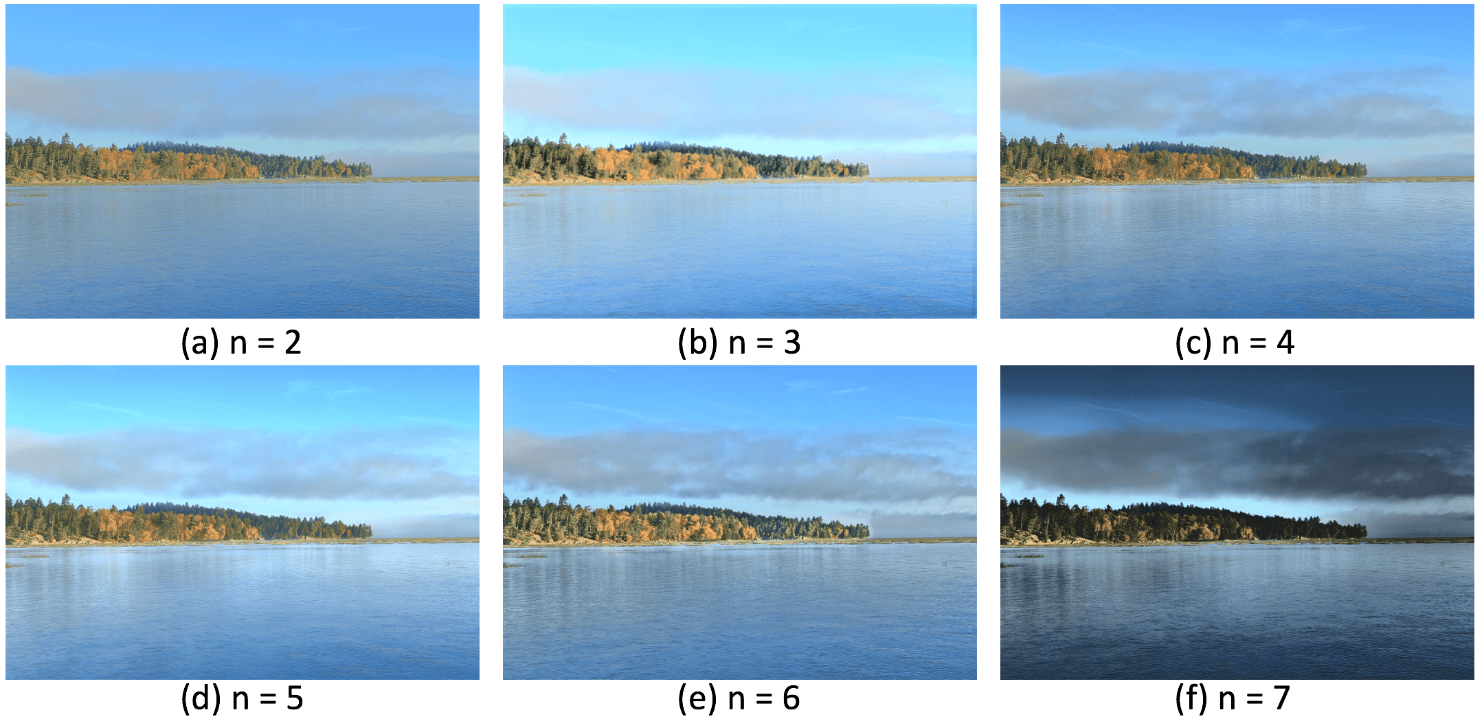
Additionally, the low-resolution input of can significantly reduce the required computation for training the parameter . Figure 4 shows the visual comparison with different choices of the number of the frequency band .
However, the generated Laplacian pyramid also has certain drawbacks. Firstly, there are layers of images and each contains different frequency components of the original WDR image. It would be difficult to process all different layers with a single neural network because the low frequency layer needs to be compressed greatly while the high frequency layers only need to be manipulated locally. Furthermore, if the layers are processed with different neural networks, the complexity of tone mapping model will also grow and make it not feasible to fit in hardware devices.

To overcome the mentioned drawbacks caused by the Laplacian pyramid, we reconstruct an image from the entire Laplacian pyramid without the lowest frequency layer. The generated is a single image that has the same resolution as the original WDR image. Now, the Laplacian pyramid is reformulated into two layers with representing all high frequency components and representing low frequency global luminance terrain. Figure 5 intuitively shows the relationship and the difference between the reformulated Laplacian pyramid and the original one. Using two layers in the Laplacian pyramid structure has the following advantages. First, it reduces the original Laplacian pyramid model from layers to layers, hence the computation complexity of subsequent processing is significantly reduced. Secondly, the segmentation of high and low frequency components of the WDR image leads network and to focus on simple tasks, namely, global compression and local detail manipulation, respectively.
III-B Global Compression Network
The global compression network of focuses on the compression of the global dynamic range of the WDR image, namely . After the decomposition of the Laplacian pyramid, is a low resolution image and only contains global luminance information of the original WDR image. Unlike many image transformation works [42, 29, 43] that employ encode-decode architecture to avoid the loss of the global feature during convolution, our architecture is able to achieve the same effect with the help of the low resolution representation . A small kernel is able to cover pixels of the original WDR image if the WDR image is decomposed to layers. Therefore, we adopt a simple CNN architecture to do the compression. The detail of the proposed global compression network is summarized Table I.
and are the width and height of the input image , respectively. Given an input image , and the ground truth WDR-LDR image , we use the -norm, feature loss and regularization as the loss function:
| (4) |
where = 0.5, = 0.5 and = 0.2. The -norm can be formulated as:
| (5) |
where is the lower frequency part of the corresponding reformulated Laplacian pyramid of ground truth . As our dataset is not ample comparing to all WDR image representations, we implement regularization loss to all our neural networks to prevent over-fitting.

III-C Local Manipulation Network
The purpose of the local manipulation network is to manipulate the high frequency part of the WDR image, namely . Unlike , the high frequency features contained in are mostly local. For simplicity, we adopt the same architecture in Table I to do the local manipulation. This is because has the same resolution as the WDR image, the kernels in Table I will only cover a local image patch instead of a global area. The same network can serve two different goals when cooperated with and , respectively. The learning objective of the local manipulation network and the global compression network are the same. We use the same set of parameters and loss function:
| (6) |
is the high frequency part of the corresponding reformulated Laplacian pyramid of the ground truth .
| Layers | Input Size | Kernel Size | Stride | Kernel Num. |
|---|---|---|---|---|
| Input | - | - | - | |
| Conv_1 | ||||
| Batch_norm_1 | - | - | - | |
| Conv_2 | ||||
| Batch_norm_2 | - | - | - | |
| Conv_3 | ||||
| Batch_norm_3 | - | - | - | |
| Conv_4 | ||||
| Batch_norm_4 | - | - | - | |
| Conv11 | - | - | ||
| Output | Input + Conv11 | |||
III-D Fine Tune Network
The global compression network and the local manipulation network are able to generate the corresponding reformulated Laplacian layer and , respectively. The Laplacian pyramid requires additional operations to add all frequency layers. That is, = upsampling() + . However, image cannot guarantee overall visual quality since and are produced with separate neural networks. Moreover, color shifts, regional blurry and other artifacts may also occur in .
To overcome these possible issues, we utilize a fine tune network to further refine the reconstructed image to the desired ground truth image. is a ResNet architecture with large feature maps and small depth since the main feature of the image has been learned from the previous two neural networks.
The ResNet contains 4 residual blocks. Each residual block consists of 2 convolutional layers. We use kernels for every layer with stride of 1, and we use a batch normalization layer after each convolutional layer. At the end of this ResNet, a convolution layer is applied to condense all extracted features from the 32-channel receptive field to 1. The loss function of fine tune network is slightly different than the previous network. We adopted feature loss and -norm:
| (7) |
where = 0.6 and = 0.4.
IV Experiments
In this section, we first present the experimental setup and then analyze the effects of the proposed Laplacian pyramid reformation. We then compare the proposed model with the state-of-the-art methods on two databases.
IV-A Training Data Generation
We trained the proposed network for WDR tone mapping on Laval indoor dataset [44]. This dataset contained 2,233 high-resolution (), high dynamic range indoor panoramas WDR images captured by Canon 5D Mark III camera. In the Laval indoor dataset, some images contain watermarks of different scale in the bottom region. We discard the bottom 15% of the panoramas to remove watermarks on the original images. After this cropping, the image resolution became . And the total number of images used in the experiment was 2,125. These images are further down-sampled to one-quarter of its original resolution and transferred to luminance image. The luminance image is generated and recovered using methods described in [8]. We generate 20 sub-images from each training sample. The size of the sub-images are drawn uniformly from the range [20%, 60%] of the size of an input WDR image and re-sampled to pixels The ground truth WDR-LDR images are generated using various tools including Luminance HDR 111https://github.com/LuminanceHDR/LuminanceHDR, HDR tool box provided by [45], Photoshop with human tuning and supervision.


IV-B Ground Truth Generation
Similar to Cai’s [49] reference image generation method, we generated high-quality ground truth images using several TMOs and human tuning. We used 6 TMOs in this process including Fattal [4], Ferradans [46], Mantiuk [35], Drago [50], Durand [5], and Reinhard [51] from Luminance HDR and HDR tool box. Then we employed 4 volunteers and 2 photographers in this process. The two photographers first picked out the images they thought were unsatisfactory (such as too dark, too bright, or exists distortion), and used Photoshop to fix them according to their own preferences. The volunteers performed the random pairwise comparison independently in the 7 sets of tone mapped images by given instruction:
-
•
Select one image of two that best suits your visual preferences.
-
•
Spend no more than 5 sec for each pair.
Images with the same vote or that couldn’t be selected within 5 seconds will be circulated back to photographers to modify, and then send to volunteers in the next round until all images have been selected.
IV-C Implementation Details
We randomly selected 70% images for training our model and use the remaining 10% for validation and 20% for testing. The network parameters are initialized using the truncated normal initializer. All training experiments are performed using the TensorFlow222https://www.tensorflow.org/?hl=zh-cn deep learning library. We adopt the ADAM optimizer for loss minimization with the learning rate is , momentum = 0.9 and = 0.999, . We use mini-batch gradient descent with batch size 8 for local manipulation, 64 for global compression and 4 for fine tuning. The forgoing networks are trained in multiple steps. The network and are trained first. And then, we use the loss function of to jointly train the entire system containing , and . The proposed model is trained in an end-to-end fashion.
IV-D Parameter Setting
The process of Laplacian pyramid reformulation described in Section III-A has a hidden parameter which indicates the number of layers during the original Laplacian decomposition. A different value will certainly affect the training and lead to different results. In order to evaluate the effect of this parameter on the final trained model, we trained our model with and evaluated the average PSNR, SSIM [41] and FSITM [52] on the test data set. The result is summarized in Table II. It is not surprising that the median values achieve average higher metrics. Actually, a smaller value will assign most information to the image while a larger value will move more frequency bands to . Suppose is so large that has only one pixel, then the final image will solely be determined by . On the other hand, if is too small, then will contain limited information which deteriorates the desired functionality of . The model with gives the highest metric values. In the rest of this paper, we set for all remaining experiments.


| Parameter | PSNR (dB) | SSIM | FSITM |
|---|---|---|---|
| 17.4065 | 0.8586 | 0.8983 | |
| 17.2129 | 0.8475 | 0.9209 | |
| 19.2187 | 0.8417 | 0.9212 | |
| 19.6627 | 0.8782 | 0.9321 | |
| 20.0335 | 0.8948 | 0.9378 | |
| 16.7248 | 0.7996 | 0.9195 |
IV-E Running Time
We report the processing time of each algorithm in Table III. We evaluated all methods on a PC with Intel(R) Core(TM) i5-8600 CPU 3.10GHz, 16G memory. We used one HDR image of size as input. Note that learning-based TM solutions are designed under GPU environment by convention since they run often significantly slower than other TM approaches under CPU environment. Our model runs 24.95 seconds with CPU and 0.61 seconds with GPU (Nvidia Titan Xp).


IV-F Comparison With State-of-the-art Methods
We compare the proposed model with other 6 state-of-the-art image tone mapping methods, namely, Gu TMO [8], Mantiuk TMO [35], Paris TMO [7], Ferradans TMO [46], Mai TMO [47], and Photomatix TMO [48]. Among them, Gu TMO [8] is based on edge preserving filter theory, images tone mapped with this TMO usually exhibit more detail. Paris TMO [7] is based on local Laplacian operator and it is good at preserving details from the WDR image. Mantiuk TMO [35] regards tone mapping as an optimization problem, though it has some difficulty in preserving detail, it can give very natural looking image results. Ferradans TMO [46] and Mai TMO [47] are popular tone mapping methods and are used in open source applications. Photomatix is a commercial software dedicated to WDR image tone mapping.
The following results of the mentioned algorithms are obtained from their online websites or open source projects with default parameter settings. We evaluate the model on the test dataset first and then on a totally different database.
IV-F1 Objective Quality Assessment
We first compared our algorithm with these methods on images from the test set of the Laval database. The results on one image are shown in Figure 6. All methods are able to produce acceptable images. However, they also have different problems.
For example, images obtained with Mantiuk TMO, Paris TMO, Ferradans TMO, and Photomatix TMO are generally darker than other images which give them a disadvantage for screening and human observing. Mai TMO generates the brightest image but it also saturates the area within the red rectangle. Both Gu TMO and the proposed method are able to generate images that are similar to the reference image. However, the image from the proposed TMO looks more natural than the image of Gu TMO because of the global luminance distribution. Moreover, it can display more local detail in the floor when compared with the Gu TMO.
Actually, the proposed model is able to extract local detail even under some extreme conditions. Two examples are given in Figure 7. The two images show a commonly seen WDR scenario where there is extreme luminance difference between inside and outside window area. The proposed model can still display the scenes outside the window more clearly than other results including the reference images.
| Methods | PSNR | SSIM | FSITM | HDR-VDP2 |
|---|---|---|---|---|
| Gu [8] | 16.5024 | 0.7755 | 0.830 | 35.165 |
| Mantiuk [35] | 14.8641 | 0.7563 | 0.876 | 38.864 |
| Paris [7] | 18.3214 | 0.8443 | 0.853 | 39.598 |
| Ferradans [46] | 16.7242 | 0.8756 | 0.863 | 39.219 |
| Mai [47] | 19.4638 | 0.8842 | 0.858 | 39.346 |
| Photomatrix [48] | 17.0730 | 0.8565 | 0.856 | 42.194 |
| Ours | 20.0335 | 0.8948 | 0.864 | 42.215 |
| Methods | TMQI | BTMQI | FSITM | HDR-VDP2 |
|---|---|---|---|---|
| Gu [8] | 0.8300 | 3.6683 | 0.823 | 26.161 |
| Mantiuk [35] | 0.9194 | 3.7474 | 0.872 | 27.686 |
| Paris [7] | 0.9228 | 2.8849 | 0.857 | 26.747 |
| Ferradans [46] | 0.8418 | 4.4286 | 0.857 | 27.35 |
| Mai [47] | 0.8894 | 3.8959 | 0.859 | 27.464 |
| Photomatrix [48] | 0.8978 | 3.3978 | 0.869 | 27.226 |
| Ours | 0.9257 | 4.5110 | 0.868 | 29.323 |
PSNR, SSIM, FSITM and HDR-VDP2 [53] are employed to assess these algorithms quantitatively. FSITM is designed to evaluate the feature similarity index for tone-mapped images. We measured the quality of the images using HDR-VDP2, the visual metric that mimics the anatomy of the HVS to evaluate the quality of HDR images. The average indices obtained from the test set of Laval database is summarized in Table IV. In all four metrics, the proposed algorithm is able to achieve the highest scores for PSNR, SSIM and HDR-VDP2. For the FSITM, the algorithm achieves the second highest score.
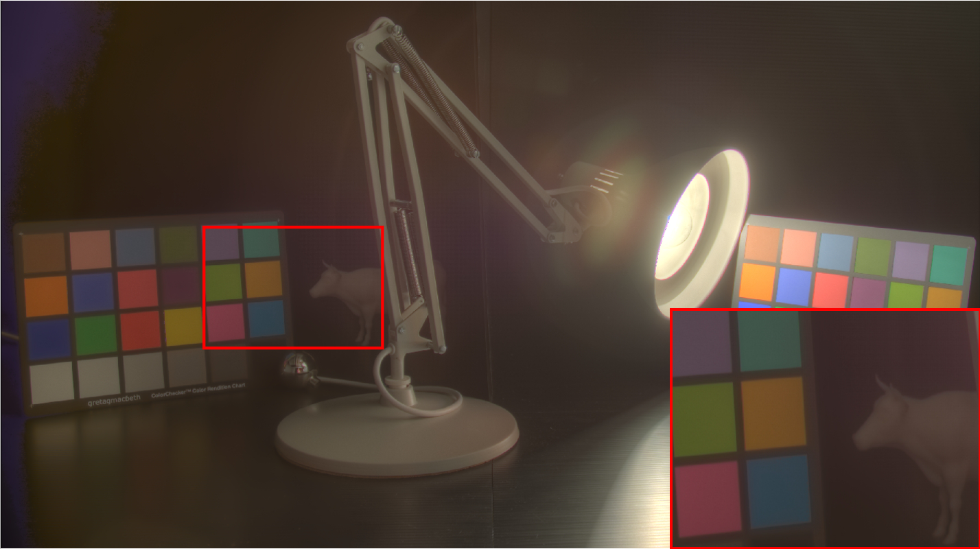
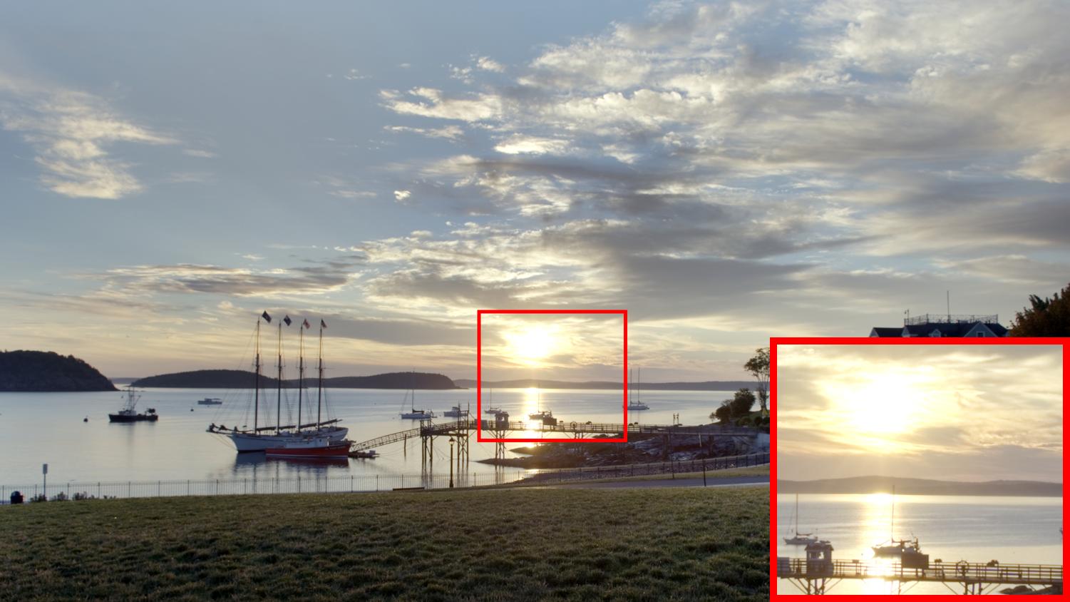
To further demonstrate the robustness of our method, we evaluate our method on images outside the test set. We choose Fairchild database [54] which contains 105 WDR images containing various situations. It is a commonly used benchmark for measuring tone mapping methods. Two result images are shown in Figure 8. The first image has a very wide dynamic range in front of and behind the lamp. Mantiuk TMO, Ferrandans TMO, Mai TMO, and the proposed models are able to generate images while other algorithms show various color artifacts in the top left dim region. In the four images without artifacts, the proposed model is able to show the color boards clearly under both dark and bright lighting conditions. In the second image, only Gu TMO and the proposed model are able to show clearly the shape of the sun. Images obtained with other methods cannot show this detail. Since there are no reference images for Fairchild database, we use the blind quality indexes alone with TMQI [55] to quantitatively measure the performance of different methods. Blind quality assessment of tone mapped images (BTMQI) [56] are two blind metrics that do not require a reference image to compute a metric score. The computed indices are summarized in Table V. The proposed model is able to achieve the highest TMQI and BTMQI scores.
| Ferradans [46] | 69 | 8.625 | 6.184 |
|---|---|---|---|
| Gu [8] | 111 | 13.875 | 6.403 |
| Mai [47] | 65 | 8.125 | 6.571 |
| Mantiuk [35] | 54 | 6.75 | 6.079 |
| Paris [7] | 52 | 6.5 | 5.586 |
| Photomatrix [48] | 39 | 4.875 | 5.642 |
| Ours | 112 | 14 | 6.580 |
IV-F2 Subjective Preference Assessment
We used human-preferred tuning to generate our ground truth images. In this process, no metrics were employed because no golden standard metrics exist to evaluate the quality of a tone mapped image nor do the metrics truly reflect the observers’ preference. These metrics can only be used as limited references. To assess the actual visual experience of our tone mapped LDR images, we also carried out a subjective preference experiment beyond the set of objective indices measurement to assess the visual quality of the image generated from our deep learning solution.
The subjective experiment has two sections: Comparative Selection Section and Image Quality Rating Section. Each section contains 8 groups of tone mapped LDR images. In the Comparative Selection Section, each group contains the LDR images generated by all 7 algorithms from the same scene for visual comparison. Participants were asked to select one image of their visual preference. In the Image Quality Rating Section, participants were asked to rate each LDR image from to based on the degree of visual comfort and the degree of details revealed in the image. Details refer to the brightness, contrast, and the extent to which overexposure and underexposure details are revealed. represents “dislike” or “fuzzy details” and stands for “most favorite” or “clear and rich details”. is somewhat in the middle. All images were randomly selected from Laval HDR dataset.
We used SurveyHero333https://www.surveyhero.com website to build our subjective experiment project. We send the survey invitation randomly via email, social networking websites, and application (see appendix for the experiment details). The survey result is shown in Table VI. In terms of visual experience that meant to be tested in the Comparative Selection Section, the voting results of our algorithm and Gu’s algorithm are significantly better than other approaches. The good visual experience comes from the low frequency layer that our Global Compression Network can effectively learn from the global luminance terrain of the human-tuned ground truth image. In the Image Quality Rating Section, the Local Manipulation Network in our model can extract and enhance the local high frequency details, therefore avoiding the lack of details in the overexposed and underexposed areas of the image after tone mapping. Our result achieves the highest voting score in both sections.
V Conclusion
In this work, we have proposed a new tone mapping method that can perform high-resolution WDR image tone mapping. To preserve the global low frequency feature as well as maintain local high frequency detail, we have proposed a novel reformulated Laplacian method to decompose a WDR image into a low-resolution image which contains the low frequency component of the WDR image and a high-resolution image which contains the remaining higher frequencies of the WDR image. The two images are processed by a dedicated global compression network and a local manipulation neural network, respectively. The global compression network learns how to compress the global scale gradient of a WDR image and the local manipulation network learns to manipulate local features. The generated images from the two networks are further merged together to produce the final output image for screen display. We visually and quantitatively compared our model with other state-of-the-art tone mapping methods with images from and outside the targeted database. The results showed that the proposed method outperforms other methods, and sometimes even shows better results than the ground truth.
References
- [1] O. Yadid-Pecht and E. R. Fossum, “Wide intrascene dynamic range cmos aps using dual sampling,” IEEE Transactions on Electron Devices, vol. 44, no. 10, pp. 1721–1723, 1997.
- [2] A. Spivak, A. Belenky, A. Fish, and O. Yadid-Pecht, “Wide-dynamic-range cmos image sensors—comparative performance analysis,” IEEE transactions on electron devices, vol. 56, no. 11, pp. 2446–2461, 2009.
- [3] P. E. Debevec and J. Malik, “Recovering high dynamic range radiance maps from photographs,” in Proceedings of the 24th annual conference on Computer graphics and interactive techniques. ACM Press/Addison-Wesley Publishing Co., 1997, pp. 369–378.
- [4] R. Fattal, D. Lischinski, and M. Werman, “Gradient domain high dynamic range compression,” in ACM transactions on graphics (TOG), vol. 21, no. 3. ACM, 2002, pp. 249–256.
- [5] F. Durand and J. Dorsey, “Fast bilateral filtering for the display of high-dynamic-range images,” in ACM transactions on graphics (TOG), vol. 21, no. 3. ACM, 2002, pp. 257–266.
- [6] E. Reinhard and K. Devlin, “Dynamic range reduction inspired by photoreceptor physiology,” IEEE Transactions on Visualization & Computer Graphics, no. 1, pp. 13–24, 2005.
- [7] S. Paris, S. W. Hasinoff, and J. Kautz, “Local laplacian filters: edge-aware image processing with a laplacian pyramid,” Communications of the ACM, vol. 58, no. 3, pp. 81–91, 2015.
- [8] B. Gu, W. Li, M. Zhu, and M. Wang, “Local edge-preserving multiscale decomposition for high dynamic range image tone mapping,” IEEE Transactions on image Processing, vol. 22, no. 1, pp. 70–79, 2013.
- [9] K. Zhang, W. Zuo, Y. Chen, D. Meng, and L. Zhang, “Beyond a gaussian denoiser: Residual learning of deep cnn for image denoising,” IEEE Transactions on Image Processing, vol. 26, no. 7, pp. 3142–3155, 2017.
- [10] C. Dong, C. C. Loy, K. He, and X. Tang, “Image super-resolution using deep convolutional networks,” IEEE transactions on pattern analysis and machine intelligence, vol. 38, no. 2, pp. 295–307, 2016.
- [11] O. Ronneberger, P. Fischer, and T. Brox, “U-net: Convolutional networks for biomedical image segmentation,” in International Conference on Medical image computing and computer-assisted intervention. Springer, 2015, pp. 234–241.
- [12] R. Zhang, P. Isola, and A. A. Efros, “Colorful image colorization,” in European Conference on Computer Vision. Springer, 2016, pp. 649–666.
- [13] J. Johnson, A. Alahi, and L. Fei-Fei, “Perceptual losses for real-time style transfer and super-resolution,” in European Conference on Computer Vision. Springer, 2016, pp. 694–711.
- [14] L. A. Gatys, A. S. Ecker, and M. Bethge, “Image style transfer using convolutional neural networks,” in Proceedings of the IEEE Conference on Computer Vision and Pattern Recognition, 2016, pp. 2414–2423.
- [15] H. Noh, S. Hong, and B. Han, “Learning deconvolution network for semantic segmentation,” in Proceedings of the IEEE international conference on computer vision, 2015, pp. 1520–1528.
- [16] J. Long, E. Shelhamer, and T. Darrell, “Fully convolutional networks for semantic segmentation,” in Proceedings of the IEEE conference on computer vision and pattern recognition, 2015, pp. 3431–3440.
- [17] Y.-H. Tsai, X. Shen, Z. Lin, K. Sunkavalli, X. Lu, and M.-H. Yang, “Deep image harmonization,” in IEEE Conference on Computer Vision and Pattern Recognition (CVPR), vol. 2, 2017.
- [18] Y. S. Heo, K. M. Lee, S. U. Lee, Y. Moon, and J. Cha, “Ghost-free high dynamic range imaging,” in Asian Conference on Computer Vision. Springer, 2010, pp. 486–500.
- [19] C. Lee, Y. Li, and V. Monga, “Ghost-free high dynamic range imaging via rank minimization,” IEEE Signal Processing Letters, vol. 21, no. 9, pp. 1045–1049, 2014.
- [20] P. Sen, N. K. Kalantari, M. Yaesoubi, S. Darabi, D. B. Goldman, and E. Shechtman, “Robust patch-based hdr reconstruction of dynamic scenes.” ACM Trans. Graph., vol. 31, no. 6, pp. 203–1, 2012.
- [21] S. Wu, J. Xu, Y.-W. Tai, and C.-K. Tang, “Deep high dynamic range imaging with large foreground motions,” in European Conference on Computer Vision. Springer, 2018, pp. 120–135.
- [22] F. Banterle, P. Ledda, K. Debattista, and A. Chalmers, “Inverse tone mapping,” in Proceedings of the 4th international conference on Computer graphics and interactive techniques in Australasia and Southeast Asia. ACM, 2006, pp. 349–356.
- [23] A. G. Rempel, M. Trentacoste, H. Seetzen, H. D. Young, W. Heidrich, L. Whitehead, and G. Ward, “Ldr2hdr: on-the-fly reverse tone mapping of legacy video and photographs,” in ACM transactions on graphics (TOG), vol. 26, no. 3. ACM, 2007, p. 39.
- [24] R. P. Kovaleski and M. M. Oliveira, “High-quality brightness enhancement functions for real-time reverse tone mapping,” The Visual Computer, vol. 25, no. 5-7, pp. 539–547, 2009.
- [25] T.-H. Wang, C.-W. Chiu, W.-C. Wu, J.-W. Wang, C.-Y. Lin, C.-T. Chiu, and J.-J. Liou, “Pseudo-multiple-exposure-based tone fusion with local region adjustment,” IEEE Transactions on Multimedia, vol. 17, no. 4, pp. 470–484, 2015.
- [26] Y. Endo, Y. Kanamori, and J. Mitani, “Deep reverse tone mapping.” ACM Trans. Graph., vol. 36, no. 6, pp. 177–1, 2017.
- [27] G. Eilertsen, J. Kronander, G. Denes, R. K. Mantiuk, and J. Unger, “Hdr image reconstruction from a single exposure using deep cnns,” ACM Transactions on Graphics (TOG), vol. 36, no. 6, p. 178, 2017.
- [28] D. Marnerides, T. Bashford-Rogers, J. Hatchett, and K. Debattista, “Expandnet: A deep convolutional neural network for high dynamic range expansion from low dynamic range content,” in Computer Graphics Forum, vol. 37, no. 2. Wiley Online Library, 2018, pp. 37–49.
- [29] S. Lee, G. H. An, and S.-J. Kang, “Deep recursive hdri: Inverse tone mapping using generative adversarial networks,” in Proceedings of the European Conference on Computer Vision (ECCV), 2018, pp. 596–611.
- [30] J. Tumblin and H. Rushmeier, “Tone reproduction for realistic images,” IEEE Computer graphics and Applications, vol. 13, no. 6, pp. 42–48, 1993.
- [31] G. Ward, “A contrast-based scalefactor for luminance display,” Graphics gems IV, pp. 415–421, 1994.
- [32] I. R. Khan, S. Rahardja, M. M. Khan, M. M. Movania, and F. Abed, “A tone-mapping technique based on histogram using a sensitivity model of the human visual system,” IEEE Transactions on Industrial Electronics, vol. 65, no. 4, pp. 3469–3479, 2018.
- [33] J. H. Van Hateren, “Encoding of high dynamic range video with a model of human cones,” ACM Transactions on Graphics (TOG), vol. 25, no. 4, pp. 1380–1399, 2006.
- [34] H. Spitzer, Y. Karasik, and S. Einav, “Biological gain control for high dynamic range compression,” in Color and Imaging Conference, vol. 2003, no. 1. Society for Imaging Science and Technology, 2003, pp. 42–50.
- [35] R. Mantiuk, S. Daly, and L. Kerofsky, “Display adaptive tone mapping,” in ACM Transactions on Graphics (TOG), vol. 27, no. 3. ACM, 2008, p. 68.
- [36] K. Ma, H. Yeganeh, K. Zeng, and Z. Wang, “High dynamic range image tone mapping by optimizing tone mapped image quality index,” in Multimedia and Expo (ICME), 2014 IEEE International Conference on. IEEE, 2014, pp. 1–6.
- [37] Z. Farbman, R. Fattal, D. Lischinski, and R. Szeliski, “Edge-preserving decompositions for multi-scale tone and detail manipulation,” in ACM Transactions on Graphics (TOG), vol. 27, no. 3. ACM, 2008, p. 67.
- [38] G. Eilertsen, R. K. Mantiuk, and J. Unger, “A comparative review of tone-mapping algorithms for high dynamic range video,” in Computer Graphics Forum, vol. 36, no. 2. Wiley Online Library, 2017, pp. 565–592.
- [39] M. Gharbi, J. Chen, J. T. Barron, S. W. Hasinoff, and F. Durand, “Deep bilateral learning for real-time image enhancement,” ACM Transactions on Graphics (TOG), vol. 36, no. 4, p. 118, 2017.
- [40] A. Loza, L. Mihaylova, N. Canagarajah, and D. Bull, “Structural similarity-based object tracking in video sequences,” in 2006 9th International Conference on Information Fusion. IEEE, 2006, pp. 1–6.
- [41] Z. Wang, A. C. Bovik, H. R. Sheikh, and E. P. Simoncelli, “Image quality assessment: from error visibility to structural similarity,” IEEE Trans Image Process, vol. 13, no. 4, pp. 600–612, 2004.
- [42] X. Yang, K. Xu, Y. Song, Q. Zhang, X. Wei, and R. W. Lau, “Image correction via deep reciprocating hdr transformation,” in Proceedings of the IEEE Conference on Computer Vision and Pattern Recognition, 2018, pp. 1798–1807.
- [43] J. Cai, S. Gu, and L. Zhang, “Learning a deep single image contrast enhancer from multi-exposure images,” IEEE Transactions on Image Processing, vol. 27, no. 4, pp. 2049–2062, 2018.
- [44] M.-A. Gardner, K. Sunkavalli, E. Yumer, X. Shen, E. Gambaretto, C. Gagné, and J.-F. Lalonde, “Learning to predict indoor illumination from a single image,” arXiv preprint arXiv:1704.00090, 2017.
- [45] F. Banterle, A. Artusi, K. Debattista, and A. Chalmers, Advanced High Dynamic Range Imaging (2nd Edition). Natick, MA, USA: AK Peters (CRC Press), July 2017.
- [46] S. Ferradans, M. Bertalmio, E. Provenzi, and V. Caselles, “An analysis of visual adaptation and contrast perception for tone mapping,” IEEE Transactions on Pattern Analysis and Machine Intelligence, vol. 33, no. 10, pp. 2002–2012, 2011.
- [47] Z. Mai, H. Mansour, R. Mantiuk, P. Nasiopoulos, R. Ward, and W. Heidrich, “Optimizing a tone curve for backward-compatible high dynamic range image and video compression,” IEEE transactions on image processing, vol. 20, no. 6, pp. 1558–1571, 2011.
- [48] Photomatrix, https://www.hdrsoft.com/, [Online; accessed 19-July-2018].
- [49] J. Cai, S. Gu, and L. Zhang, “Learning a deep single image contrast enhancer from multi-exposure images,” IEEE Transactions on Image Processing, vol. 27, no. 4, pp. 2049–2062, 2018.
- [50] F. Drago, K. Myszkowski, T. Annen, and N. Chiba, “Adaptive logarithmic mapping for displaying high contrast scenes,” in Computer Graphics Forum, vol. 22, no. 3. Wiley Online Library, 2003, pp. 419–426.
- [51] E. Reinhard, W. Heidrich, P. Debevec, S. Pattanaik, G. Ward, and K. Myszkowski, High dynamic range imaging: acquisition, display, and image-based lighting. Morgan Kaufmann, 2010.
- [52] H. Z. Nafchi, A. Shahkolaei, R. F. Moghaddam, and M. Cheriet, “Fsitm: A feature similarity index for tone-mapped images,” IEEE Signal Processing Letters, vol. 22, no. 8, pp. 1026–1029, 2014.
- [53] R. Mantiuk, K. J. Kim, A. G. Rempel, and W. Heidrich, “Hdr-vdp-2: A calibrated visual metric for visibility and quality predictions in all luminance conditions,” ACM Transactions on graphics (TOG), vol. 30, no. 4, pp. 1–14, 2011.
- [54] M. D. Fairchild, “The hdr photographic survey,” in Color and Imaging Conference, vol. 2007, no. 1. Society for Imaging Science and Technology, 2007, pp. 233–238.
- [55] Y. Hojatollah and W. Zhou, “Objective quality assessment of tone-mapped images,” IEEE Transactions on Image Processing A Publication of the IEEE Signal Processing Society, vol. 22, no. 2, pp. 657–667, 2013.
- [56] G. Ke, S. Wang, G. Zhai, S. Ma, X. Yang, W. Lin, W. Zhang, and G. Wen, “Blind quality assessment of tone-mapped images via analysis of information, naturalness, and structure,” IEEE Transactions on Multimedia, vol. 18, no. 3, pp. 432–443, 2016.
-A Comparative Selection
This section contains 8 questions. Each question has a group of 7 tone mapped LDR images in random order. Fig. 9 shows an example of a question. Participants can click on each image to view the full size. During the survey, participants need to choose an image with the best visual preference.

-B Image Quality Rating
This section contains 6 questions, 7 tone mapped LDR images in each question. Fig. 10 shows an example of a question. Participants are asked to rate each LDR image from 1 to 10 based on image brightness, image contrast, and the extent to which overexposure and underexposure details are revealed. 1 represents ”dislike” or ”fuzzy details” and 10 stands for ”most favorite” or ”clear and rich details”.

-C Assessment Process and Results
We send out our survey444https://surveyhero.com/c/7040d7c6 via WeChat (the Chinese social media and multipurpose application) and email. Each participant is only allowed to complete the survey once. Participants can also choose to abandon the test at any time. Until the submission of the paper, there were a total of 71 people participated in the survey. Table VII and Table VIII summarizes result of Comparative Selection and Image Quality Rating respectively.
We perform a simple averaging function to obtain in the Comparative Selection section by the equation
| (8) |
where s denotes the number of LDR images being selected from each algorithm in each question. represents the total number of questions in the Comparative Selection section.
To acquire the in the Image Quality Rating section, we first computed the weighted average score of each TMO by the equation
| (9) |
where denote each rating score (from 1 to 10). is the number of score that participants rated to the LDR image.
Then we used to calculate the
| (10) |
where represents the total number of questions in the Image Quality Rating section.
| Methods | 1 | 2 | 3 | 4 | 5 | 6 | 7 | 8 | ||
|---|---|---|---|---|---|---|---|---|---|---|
| Ferradans [46] | 8 | 4 | 7 | 10 | 8 | 14 | 9 | 9 | 69 | 8.625 |
| Gu [8] | 16 | 25 | 9 | 13 | 18 | 8 | 11 | 11 | 111 | 13.875 |
| Mai [47] | 15 | 7 | 8 | 8 | 5 | 7 | 9 | 6 | 65 | 8.125 |
| Mantiuk [35] | 3 | 6 | 10 | 11 | 7 | 9 | 4 | 4 | 54 | 6.75 |
| Paris [7] | 8 | 4 | 17 | 9 | 5 | 3 | 2 | 4 | 52 | 6.5 |
| Photomatix [48] | 2 | 2 | 10 | 3 | 4 | 4 | 8 | 6 | 39 | 4.875 |
| Ours | 19 | 23 | 7 | 13 | 11 | 11 | 13 | 15 | 112 | 14 |
| Methods | 1 | 2 | 3 | 4 | 5 | 6 | |
|---|---|---|---|---|---|---|---|
| Ferradans [46] | 6.45 | 5.59 | 5.47 | 6.50 | 5.87 | 7.23 | 6.18 |
| Gu [8] | 6.00 | 6.39 | 6.06 | 7.00 | 6.10 | 6.87 | 6.40 |
| Mai [47] | 6.64 | 6.29 | 6.27 | 6.73 | 6.19 | 7.31 | 6.57 |
| Mantiuk [35] | 5.88 | 6.11 | 5.73 | 6.72 | 5.52 | 6.52 | 6.08 |
| Paris [7] | 5.47 | 5.93 | 5.76 | 5.29 | 5.16 | 5.90 | 5.59 |
| Photomatix [48] | 6.00 | 5.52 | 4.55 | 6.21 | 6.10 | 5.48 | 5.64 |
| Our | 6.56 | 6.25 | 6.40 | 6.43 | 6.84 | 7.00 | 6.58 |
-D Color Recovery
Our approach operates on luminance WDR images. We employed an additional color recovery step to assign a color to the pixels of compressed dynamic range images using the method described in [4]
| (11) |
where is the final WDR-LDR output after the fine tune network. and denote the WDR image of the output and the one after dynamic range compression, respectively. We set the color saturation controller s=0.6 as [4] found to produce satisfactory results.
-E Additional Qualitative Comparisons
Figs. 11 - 16 show additional results of qualitative comparison with the state-of-the-art algorithms [35, 7, 46, 47, 8, 48]. The images were randomly chosen from the test set of Laval dataset [44]. The dataset contains uniformly panorama indoor WDR images in various scenes with the aspect ratio of around 1.0 to 2.0. To better demonstrate our model’s performance in preserving local details, we crop the full size images to half size and keep the overexposed regions. Our model is able to recover more details in these regions when compared with other state-of-the-art methods. Figs. 17 - 20 show full size output of different methods. It also yields visually comparable or better WDR-LDR images when compared with other methods. Figs. 21 - 24 show visual comparison with different choices of the number of the frequency band in the Fairchild dataset [54]. Although our neural network was trained with an indoor dataset which the dynamic range inevitably much smaller than the outdoors, our method still be able to yield pleasing WDR-LDR images.
From these exhaustive predicted outputs, we show the proposed method generates output not only effectively compress global dynamic range like other compared methods, but also preserves and enhances the details of saturated region better.