Deep Operator Networks
for Bayesian Parameter Estimation in PDEs
Abstract
We present a novel framework combining Deep Operator Networks (DeepONets) with Physics-Informed Neural Networks (PINNs) to solve partial differential equations (PDEs) and estimate their unknown parameters. By integrating data-driven learning with physical constraints, our method achieves robust and accurate solutions across diverse scenarios. Bayesian training is implemented through variational inference, allowing for comprehensive uncertainty quantification for both aleatoric and epistemic uncertainties. This ensures reliable predictions and parameter estimates even in noisy conditions or when some of the physical equations governing the problem are missing. The framework demonstrates its efficacy in solving forward and inverse problems, including the 1D unsteady heat equation and 2D reaction-diffusion equations, as well as regression tasks with sparse, noisy observations. This approach provides a computationally efficient and generalizable method for addressing uncertainty quantification in PDE surrogate modeling.
keywords:
Physics-Informed Neural Networks, Partial Differential Equations, Parameter Estimation, Machine Learning[csulb]organization=Depratment of Computer Engineering and Computer Science, addressline= California State University, city=Long Beach, postcode=90840, state=CA, country=USA
1 Introduction
The modeling and simulation of complex physical systems governed by partial differential equations (PDEs) are critical in science and engineering. Traditional numerical methods for solving PDEs, while effective, often demand substantial computational resources and face challenges with high-dimensional or nonlinear problems [1, 2]. Neural networks have emerged as promising tools for approximating PDE solutions [3, 4, 5, 6]. However, these models typically require large datasets and lack mechanisms to embed physical laws into their frameworks.
Physics-Informed Neural Networks (PINNs) [7, 8] integrate governing physical laws, expressed as PDEs, directly into their loss functions. This approach enables PINNs to solve forward and inverse problems efficiently, even with limited data, by ensuring that predictions adhere to the underlying physics. By embedding physical laws into the learning process, PINNs overcome the reliance on extensive datasets required by traditional neural networks, making them more practical for real-world scenarios [9]. Applications of PINNs include solving fluid dynamics problems [10, 11], addressing inverse problems [12, 13], controlling dynamical systems [14, 15, 16], and performing uncertainty quantification [17].
Automatic differentiation (AD) is integral to the functionality of PINNs, enabling precise and efficient computation of PDE residuals, even for mixed and high-order derivatives. Its integration into machine learning frameworks such as PyTorch [18], Jax [19], and TensorFlow [20] has significantly advanced deep learning applications in scientific domains. Comprehensive surveys on AD and its relationship to deep learning can be found in Baydin et al. [21] and Margossian [22].
In scientific machine learning, probabilistic models are highly valued for estimating noise in observational data, addressing model errors, and accounting for incomplete knowledge of the underlying physics. Viana et al. [23] highlight the evolution of scientific modeling, emphasizing the role of physics-informed neural networks in reducing computational costs and enhancing modeling flexibility. Molnar et al. [24] demonstrate the application of PINNs within a Bayesian framework to reconstruct flow fields from projection data, showcasing their ability to incorporate physics priors and improve accuracy in noisy environments. Li et al. [25] explore the challenges of solving inverse problems with PINNs, advocating for a Bayesian approach to provide robust uncertainty quantification, particularly when observations are sparse or noisy.
Bayesian Neural Networks (BNNs) [26, 27, 28] provide a probabilistic framework for uncertainty quantification by assigning distributions to network weights. While posterior estimation over BNN parameters is challenging due to high-dimensionality and non-convexity, methods such as Hamiltonian Monte Carlo (HMC) and variational inference (VI) approximate the posterior effectively, albeit at higher computational costs than maximum likelihood approaches. Yang et al. [29] introduced Bayesian Physics-Informed Neural Networks (B-PINNs), combining BNNs and PINNs to address forward and inverse PDE problems in noisy conditions. By integrating physical equations into training, B-PINNs offer a practical solution for probabilistic PDE learning tasks.
Accurately estimating PDE parameters while quantifying uncertainty remains a significant challenge, particularly in complex systems with scarce or noisy data. The high computational demands and challenges in selecting suitable priors in Bayesian approaches restrict the practical use of black-box sampling methods in scientific machine learning. This presents an opportunity for new methodologies that effectively combine physics-guided training with computationally efficient Bayesian approaches.
In this work, we propose a novel method that extends the capabilities of PINNs by integrating Bayesian methodologies with Deep Operator Networks (DeepONets) to enhance parameter estimation in PDEs. Our approach relies on variational inference: starting with a prior distribution for the unknown PDE parameters, we apply Bayesian inference to estimate the posterior distributions based on available data and physics. The DeepOperator architecture modulates the forward prediction of the solution of the PDE with inverse parameter estimation. This method offers substantial computational advantages, providing uncertainty quantification comparable to B-PINNs but with significantly reduced computational costs.
We continue our discussion in the following steps: In section 2, we detail the methodology of Bayesian Deep Operator Networks, demonstrate their application to parameter estimation in PDEs, and discuss their advantages and shortcomings compared to existing approaches. Section 3 presents experimental results on a variety of PDEs, showcasing the effectiveness of our method in solving forward and inverse problems. Finally, we discuss the implications of our findings for future research and potential applications in various scientific and engineering domains in section 4.
2 Methodology
2.1 Problem definition
We start by considering a parametrized partial differential equation (PDE), defined over time span and spatial domain :
| (1) |
may contain partial derivatives of the solution of the forms and . is the forward solution of the PDE and is assumed to be well defined with the necessary initial and boundary conditions. Given a dataset of noisy observations of at different times and positions:
| (2) |
we are interested in training a probabilistic machine learning model that simultaneously approximates and based on the data eq. 2 and the PDE eq. 1. We will start from a Bayesian formulation of this problem and derive a corresponding loss function for training the model.
The posterior distribution over the latent parameter given data is expressed as
| (3) |
where represents the prior distribution over , is the likelihood of the observed data given parameter , and is the marginal likelihood or evidence.
The likelihood term is constructed from two components: the data likelihood , which captures the relationship between the inputs and outputs , and the likelihood of the predicted solution satisfying the governing equations. The latter is achieved via the residuals of eq. 1.
Assuming independence across training data points, the joint likelihood is written as
| (4) |
The data likelihood is modeled with normal distribution:
| (5) |
where is the model output for input given latent variable , and is the observation noise variance. The log-likelihood is therefore
| (6) |
We are interested in models that, in addition to adherence to observation data, also produce likely predictions that satisfy the governing equations eq. 1. The likelihood of the residuals from the PDE is similarly modeled as:
| (7) |
where is the variance of the residual noise. can either be simplified as or modified to include other constraints such as the boundary and initial conditions. The corresponding log-likelihood of the residuals is
| (8) |
We sample the posterior in equation eq. 3 using variational inference (VI). Considering an approximate posterior distribution we minimize the Kullback-Leibler (KL) divergence:
| (9) |
Substituting eq. 3 for and rearranging terms, we obtain the well-known Evidence Lower Bound (ELBO) objective function:
| (10) |
Monte Carlo approximation of the integral in eq. 10 yields Expanding using the joint likelihood, eq. 10 becomes
| (11) |
Equation 12 can be evaluated using Monte Carlo sampling of the latent variable from the posterior . The observation and residual noise variances and can be considered constants or learned during training. This enables a flexible uncertainty quantification method that can be utilized to estimate model or data uncertainty. We experiment with different variance estimation strategies in the experiments section 3.
The KL divergence term in eq. 12 can be approximated empirically or analytically: If both the prior and the variational distribution are normally distributed, with means and variances , the KL divergence can be written as:
| (13) |
2.2 Model architecture
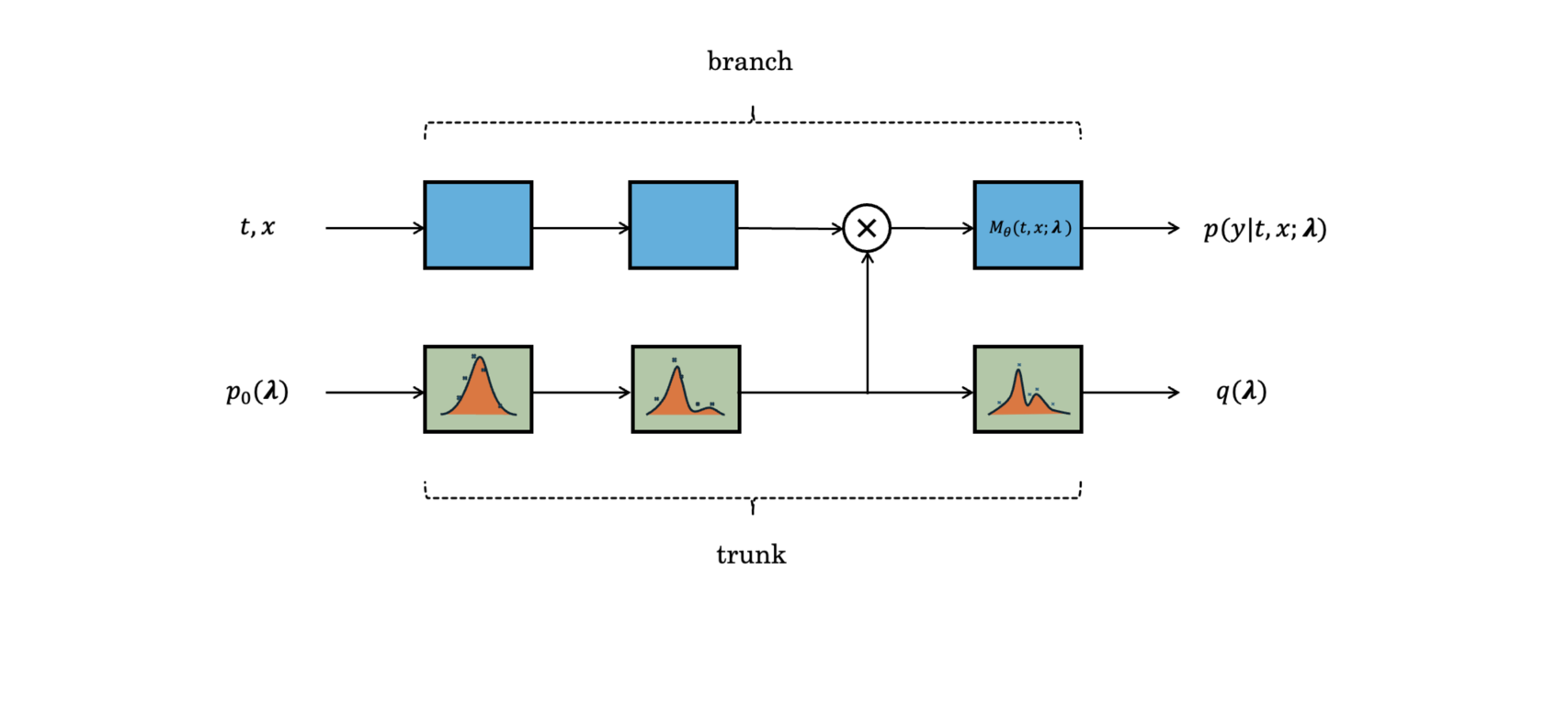
is a deep operator network (DeepONet) that consists of two components: the branch network and the trunk network [30, 31]. The branch network approximates the forward solution of the PDE. The trunk network processes independent prior samples to generate samples of the approximate posterior that also influence the branch network’s predictions. See fig. 1 for a schematic representation of the network architecture. Our proposed architectue, hereafter referred to as DeepBayONet uses the DeepONet structure to estimate the forward solution and parameters of the PDE at the same time:
| (14) |
where and are the output layer weights and bias, is the activation function, and denotes the element-wise product. The branch network and trunk network are general parametrized functions that can take the form of any neural network architectures including convolutional, recurrent, or transformer networks. The entire set of trainable parameters in the model is denoted by .
Uncertainty estimation is critical in deep neural networks, particularly in scientific modeling and prediction tasks, to assess the reliability of predictions and the robustness of the model. There are two sources of uncertainty that can be considered: Aleatoric uncertainty arises from inherent noise in the observations, reflecting variability that cannot be reduced even with additional data. This type of uncertainty is often captured by modeling the variance of the output distribution, as demonstrated in probabilistic models such as heteroscedastic neural networks [32]. In contrast, epistemic uncertainty reflects the model’s lack of knowledge or suffiecient training about the underlying data distribution and can be reduced by incorporating additional data or improving the model architecture. Bayesian neural networks (BNNs) and dropout are among various methods that cab address epistemic uncertainty [32] by learning a distribution over the model parameters, allowing the model to express uncertainty in regions of the input space the model’s predictions are ambiguous. These two sources of uncertainty provide complementary information: aleatoric uncertainty quantifies noise in the data, while epistemic uncertainty assesses the model’s confidence in its predictions.
In the proposed model, both aleatoric and epistemic uncertainties are quantified explicitly through different components of the loss function and the model’s probabilistic formulation. Aleatoric uncertainty is captured through the observation noise variance , which governs the data likelihood term in the evidence lower bound (ELBO) formulation eq. 12 where represents the variance of the observation noise. This term accounts for the inherent variability in the measurements, and by treating as a learnable parameter, the model can adaptively estimate the aleatoric uncertainty directly from the data. High values of indicate regions with significant observation noise, leading to reduced confidence in the predictions.
Epistemic uncertainty, on the other hand, is inferred from the posterior distribution over the latent parameters , as derived through variational inference. The posterior distribution is approximated by minimizing the Kullback-Leibler (KL) divergence in eq. 12. The variability in , often characterized by its variance , quantifies the model’s uncertainty about . Furthermore, the residual noise variance , associated with the residuals of the governing equation eq. 8 also contributes to epistemic uncertainty by capturing how well the predicted solutions satisfy the physical constraints imposed by the partial differential equations (PDEs).
Through Monte Carlo sampling of eq. 12, the model evaluates both aleatoric and epistemic uncertainties simultaneously, enabling a robust and interpretable quantification of uncertainty in predictions.
2.3 Relation to Dropout
A distinctive feature of the DeepBayONet architecture is the interaction between the branch and trunk networks, which not only enables the model to represent the forward solution but also plays a role in uncertainty quantification. Specifically, the branch network approximates the forward operator by mapping the inputs and to a latent feature space. Simultaneously, the trunk network processes samples of the latent parameter drawn from the approximate posterior distribution . These two networks interact through an element-wise product in eq. 14. The stochastic sampling of introduces variability in , thereby perturbing the forward operator represented by during training.
This mechanism of perturbation bears a conceptual resemblance to dropout [33], widely-used regularization as well as epistemic (model) uncertainty quantification technique in neural networks. Dropout introduces noise during training by randomly setting activations to zero with a probability sampled from a Bernoulli distribution [33]. In DeepBayONet, instead of discrete binary perturbations, the trunk network introduces continuous perturbations drawn from the posterior distribution . This continuous modulation of the branch network activations improves robustness while allowing the model to incorporate epistemic uncertainty in its predictions. Sampling from enables the model to account for uncertainty in the latent parameters . This uncertainty is propagated through the interaction between the branch and trunk networks. This continuous perturbation mechanism has two significant implications. First, it ensures that the model’s predictions generalize well by preventing the branch network from overfitting to deterministic solutions. Second, it provides a means to quantify epistemic uncertainty explicitly, as the variability in represents the model’s confidence in its parameter estimates. Thus, the DeepONet architecture naturally integrates regularization and uncertainty quantification in a unified framework, leveraging the interaction between the branch and trunk networks to achieve both objectives.
2.4 Practical Aspects of the Loss Function
The loss function defined in eq. 12 enforces adherence to the governing equations of the dynamical system while capturing uncertainties in both the observations and the parameters. To ensure practical implementation, the total loss is decomposed into distinct components, each addressing specific aspects of the problem. Assuming is the predicted PDE solution, the total loss is expressed as:
where the individual loss components are defined to correspond with the probabilistic formulation in eq. 12.
To align these loss terms with the evidence lower bound (ELBO), variance-based scaling is introduced to reflect the uncertainties in the observations and residuals. The revised definitions of the individual components are:
| (15a) | ||||
| (15b) | ||||
| (15c) | ||||
| (15d) | ||||
where is the variance of the residual noise and is the variance of the observation noise. These variances play a critical role in balancing the contributions of the individual loss terms, ensuring that the model accounts for uncertainties appropriately.
The weights and are hyperparameters used to balance the influence of the respective loss components. These weights can be selected through hyperparameter optimization or by employing adaptive weighting techniques, as explored in [34, 35]. The inclusion of variance scaling in eqs. 15a, 15b and 15c ensures consistency with the ELBO formulation, connecting the practical implementation to the probabilistic foundations of the model. This alignment also allows the model to accurately capture both aleatoric and epistemic uncertainties during training and inference.
3 Experiments
In this section, we train DeepBayONets on various algebraic and differential equations. In each case, the underlying equations have unknown parameters that are learned along with the forward dynamics. We compare the results with exact solutions and competing methodologies from the literature.
3.1 General Setup
The common configurations for all the experiments are as follows: each experiment utilizes a neural network architecture comprising three layers on both the branch and the trunk. The hyperbolic tangent () activation function is employed universally. Training and optimization are conducted using the Adam optimizer. All implementations are performed in PyTorch, leveraging its advanced features for computational graphs and gradients. Specific details, such as the number of neurons per layer, epochs, batch size, and loss weights, are tuned for each experiment based on its requirements and complexity.
3.2 Forward Bayesian Regression Problem
This experiment demonstrates DeepBayONet’s capability to estimate aleatoric and epistemic uncertainty in a synthetic regression problem. The regression task is defined as follows:
| (16) | |||||
where are noisy observations with state-dependent inhomogeneous noise. The goal is to learn the function while estimating two sources of uncertainty: Aleatoric uncertainty arising from state-dependent input noise in the data, and the epistemic uncertainty due to gaps in the data and testing outside the training range eq. 16.
The results are compared against various deep learning uncertainty quantification methods, including a Simple Neural Network with aleatoric uncertainty estimate (SNN), a Bayesian Neural Network (BNN), a Monte Carlo Dropout Network (MCDO), and a Deep Ensemble Network (DENN). Each architecture contains approximately 3,800–4,000 parameters to ensure a fair comparison. The data are split into a training set, an in-training-distribution (IDD) test set, and an out-of-training-distribution (OOD) test set.
The test problem and implementations are adopted from [36]. For a comprehensive review of uncertainty quantification methods in deep learning, refer to [37]. All networks are trained for 150 epochs with the Adam optimizer (batch size 16). Each model is run ten times with random initializations, and accuracies are averaged to mitigate random effects. Common hyperparameters are kept consistent across all models, while method-specific hyperparameters use default library values. To limit computational resource requirements, we have not done method-specific hyperparameter tuning.
We report training and testing mean squared errors (MSE) and the coverage of 95% confidence intervals (CI) predicted by the networks. This design facilitates an evaluation of both predictive accuracy and the quality of uncertainty estimates within and outside the training range.
| Architecture | MSE (mean) | MSE (std) |
|---|---|---|
| SNN | 0.147 | 0.007 |
| BNN | 0.352 | 0.008 |
| MCDO | 0.198 | 0.034 |
| DENN | 0.154 | 0.012 |
| DeepBayONet | 0.143 | 0.005 |
| Architecture | Total Testing | IDD Coverage | OOD Coverage |
|---|---|---|---|
| SNN | 63.45 | 65.92 | 48.00 |
| BNN | 13.30 | 8.57 | 21.16 |
| MCDO | 52.15 | 41.35 | 72.49 |
| DENN | 59.70 | 36.21 | 88.16 |
| DeepBayONet | 89.05 | 85.42 | 97.00 |
The results demonstrate that DeepBayONet outperforms other architectures by achieving consistently lower mean squared errors (MSE) and significantly higher confidence-interval coverage. Notably, DeepBayONet excels in out-of-training-distribution scenarios, highlighting its robustness and reliability in quantifying uncertainty across diverse testing conditions.
3.3 One-dimensional function approximation
This experiment evaluates the ability of DeepBayONet to approximate a one-dimensional function while simultaneously estimating an unknown parameter and quantifying associated uncertainties. The function to be approximated is defined as:
| (17) |
where and is an unknown parameter. For this experiment, the true value of . The dataset consists of sampled values of from the domain paired with noisy observations:
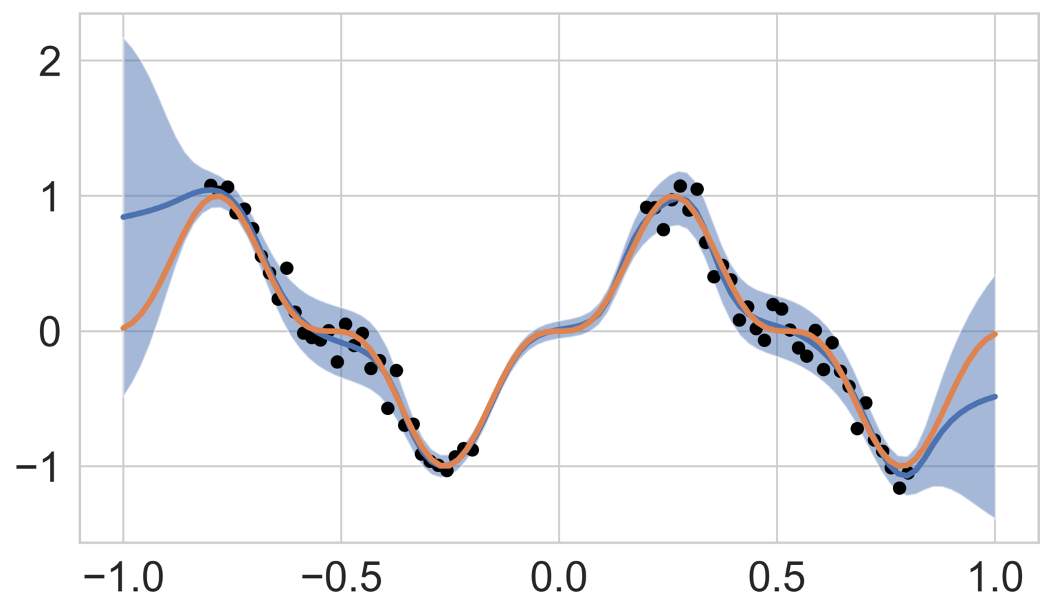
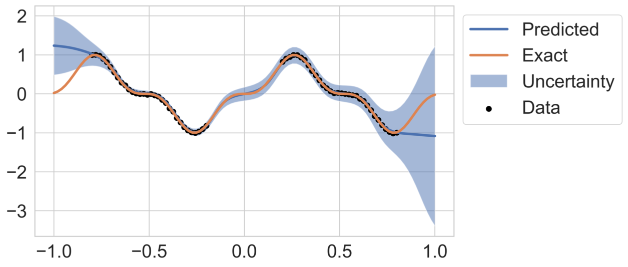
Two noise scenarios are considered: a low-noise case with and a high-noise case with .
Figure 2 shows the mean predicted function as well as the two standard deviation uncertainty bands for both high- and low-noise cases. The model demonstrates good agreement with the data within the training range, while predicting elevated uncertainty outside the training range. Higher observation noise () results in more pronounced uncertainty, reflecting the model’s ability to adapt to noisy data.
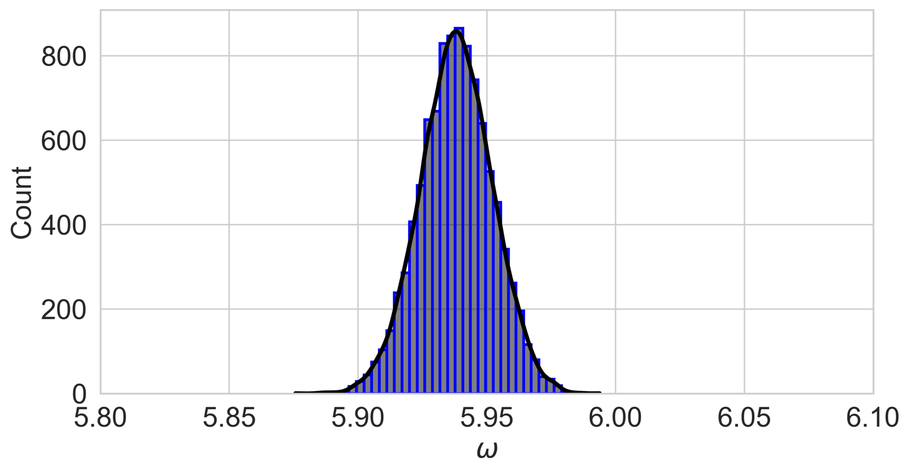
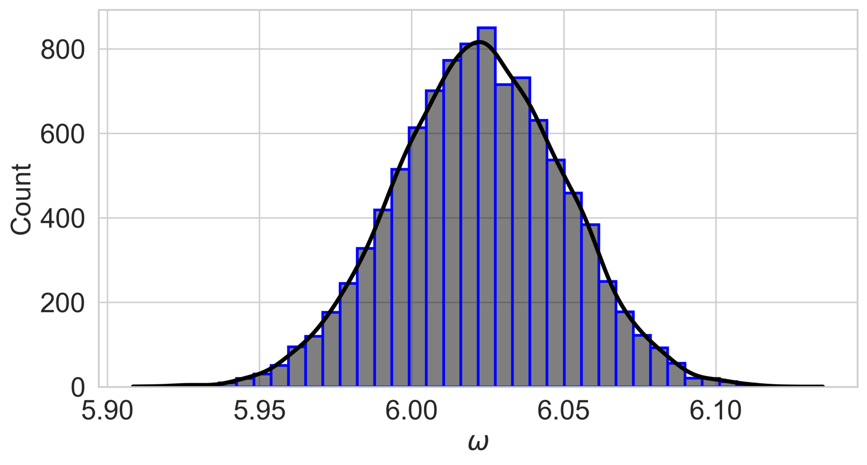
The posterior distribution of the parameter is shown in fig. 3, with the mode close to the true value of in both cases. The narrower posterior distribution in the low-noise scenario () indicates greater confidence in the parameter estimate compared to the high-noise scenario.
3.4 One-dimensional unsteady heat equation
This experiment explores DeepBayONet’s capability to solve a one-dimensional unsteady heat equation while simultaneously estimating the diffusion parameter and the decay rate . The heat equation is given as:
| (18) |
where and are unknown parameters. When and , the equation has the exact solution:
A DeepBayONet model is trained to approximate this solution while learning the parameters and . The training dataset consists of 100 spatio-temporal samples with the corresponding exact solution . A standard normal prior is used for both parameters. Training is performed for 15,000 epochs with a batch size of 100, using the Adam optimizer and an initial learning rate of 0.01. The loss component weights are configured as follows:
The model contains 2,103 trainable parameters.
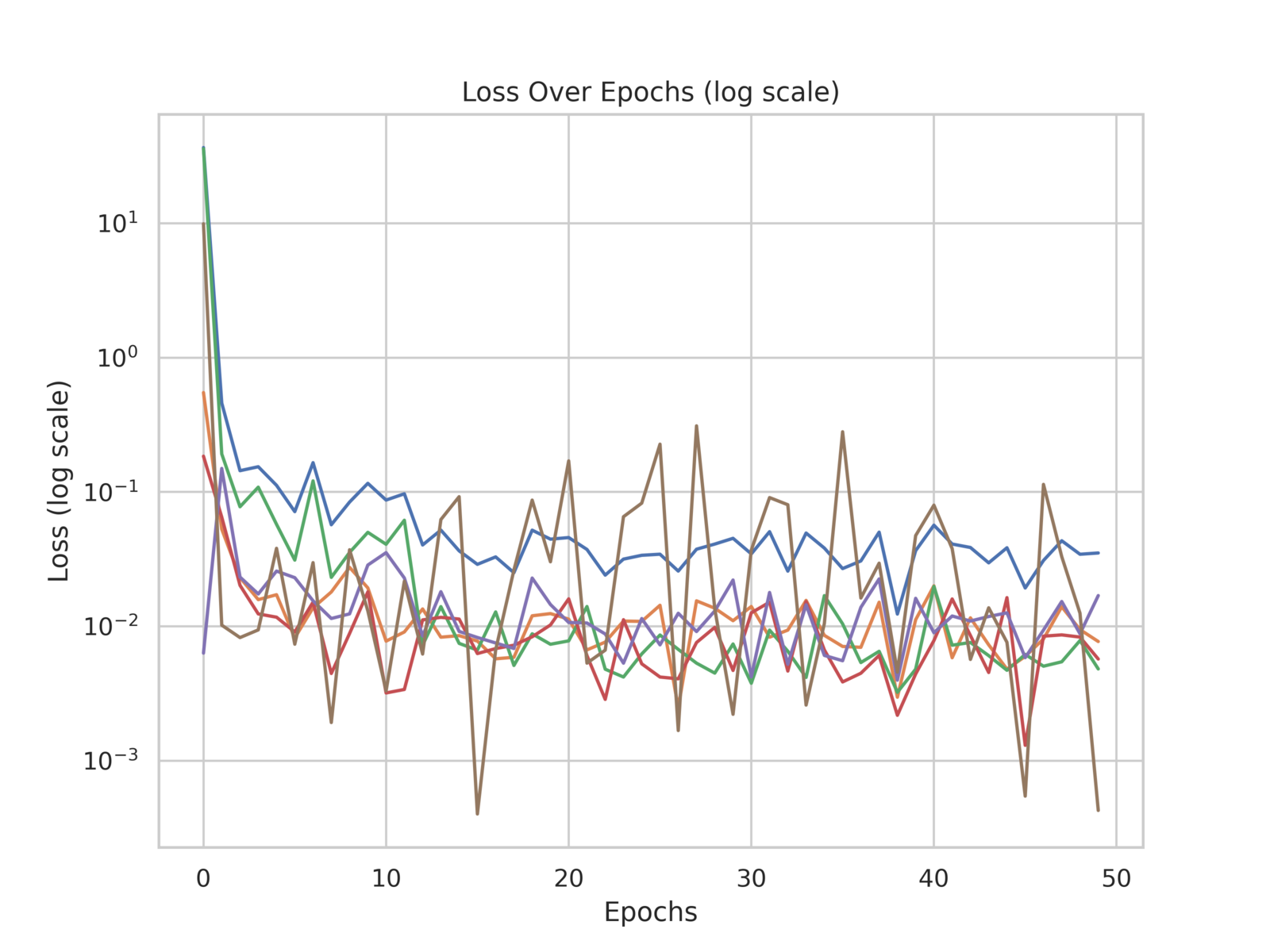
During training, several metrics were recorded to monitor the model’s performance and convergence, including the total loss and individual loss components: PDE (Interior) loss, boundary condition (BC) loss, initial condition (IC) loss, data loss, and the standard deviation loss for predicted parameters (STD loss). These metrics are shown in fig. 4, highlighting the stability and convergence of the model.
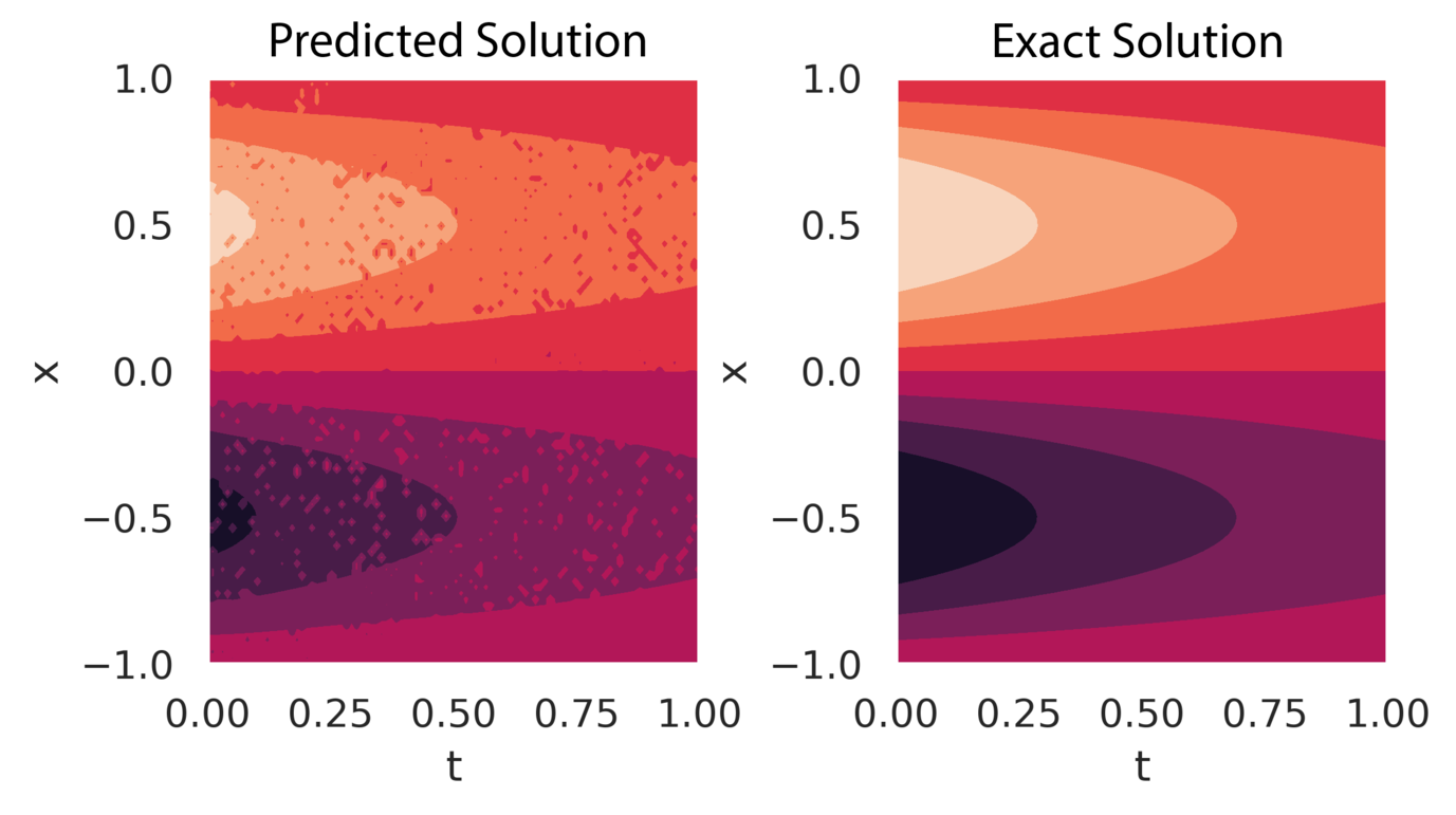
Figure 5 compares a sample of the posterior predicted solution with the exact solution. The grainy appearance of the predicted solution reflects the uncertainty in the parameters and , which affects the pointwise forward solution. However, obtaining multiple samples of the output and computing statistical measures, such as the mean and mode, is computationally efficient once the model is trained.
The histograms in fig. 6 illustrate the posterior distributions of the parameters and . The model successfully predicts these parameters, with the posterior mode aligning closely with the true values ( and ). Additionally, the secondary mode observed in the posterior distributions corresponds to larger values of and , indicating a highly diffusive and fast-decaying mode that still satisfies the PDE relatively well.
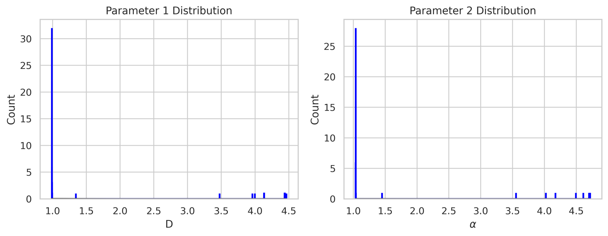
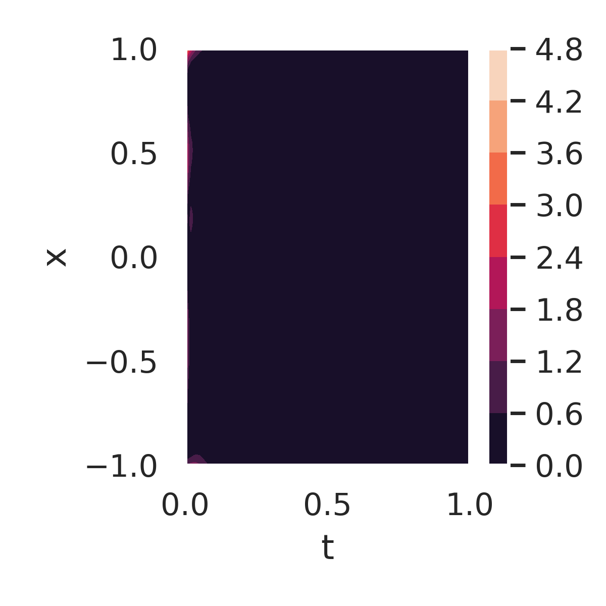
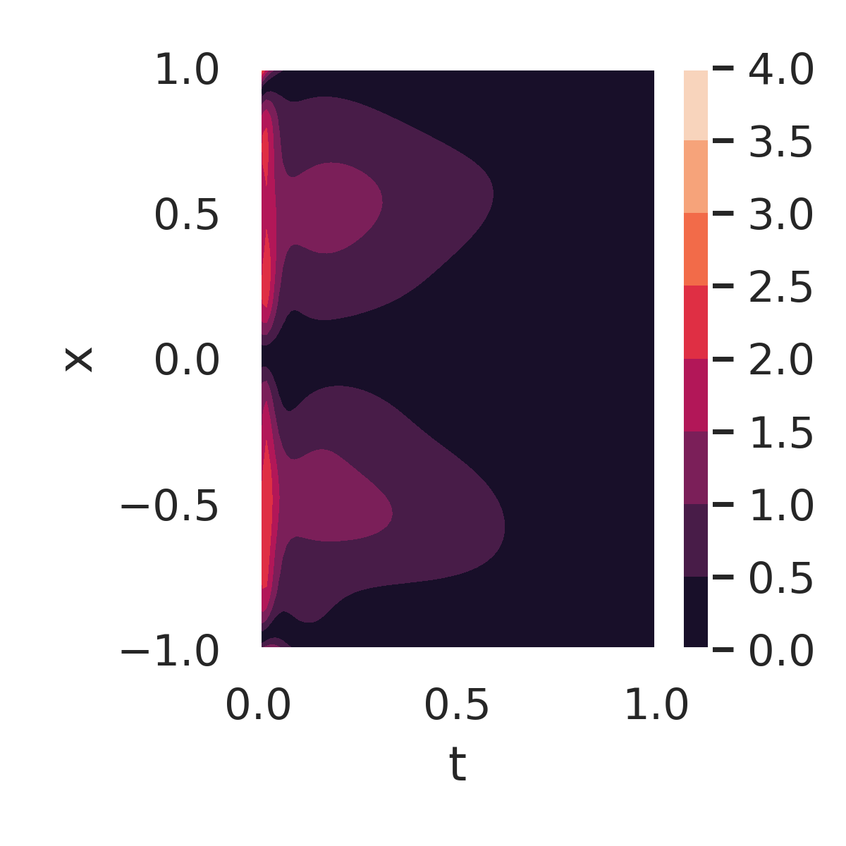
Figure 7 further examines the errors and residuals for the DeepBayONet learned solution. Figure 7a shows the absolute error compared to the exact solution when using the mean of the posterior distribution of the parameters. Small errors are observed across the domain, except near the initial condition boundaries ().
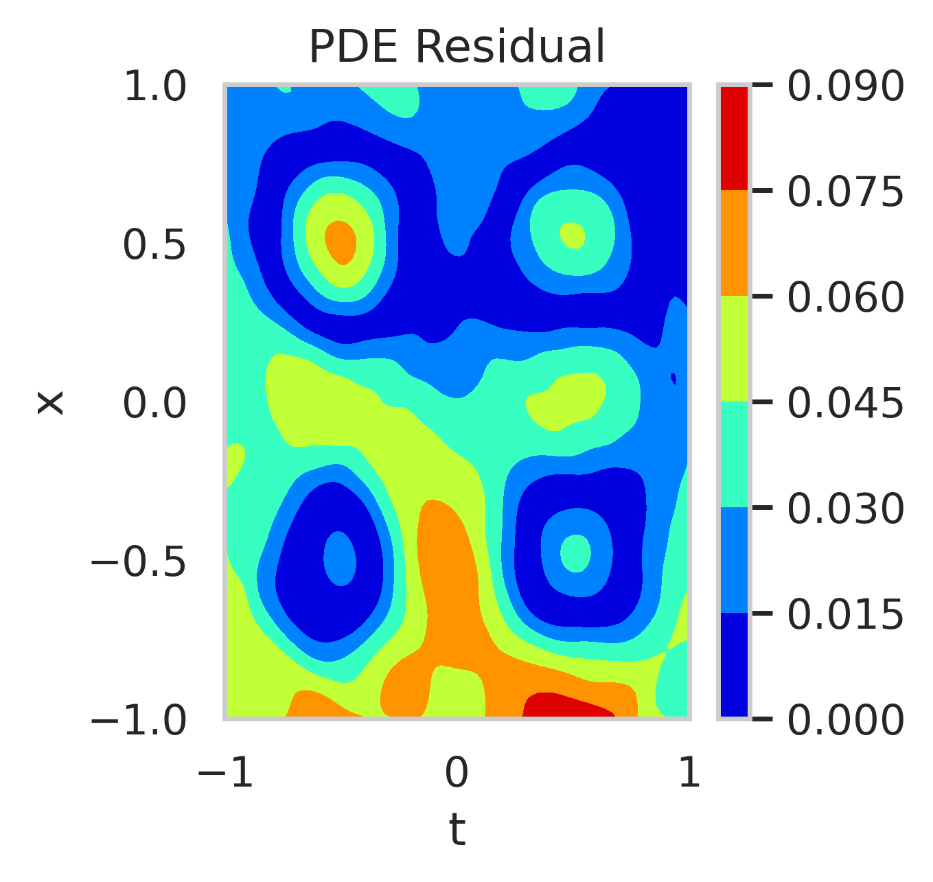
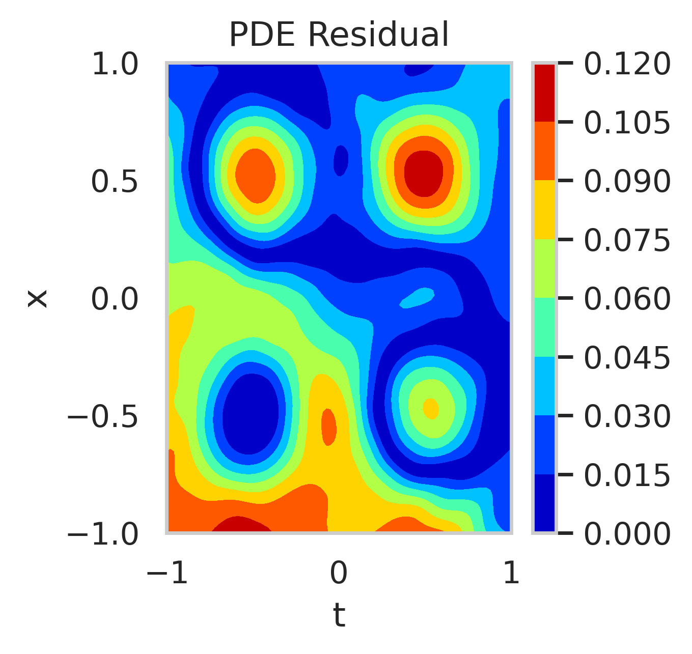
The PDE residuals, when evaluated using the primary mode (fig. 7b) and the secondary mode (fig. 7c) of the posterior distribution, provide additional insights. The secondary mode results in significantly larger residuals, reflecting suboptimal parameter values that deviate from the true solution.

3.5 Two-dimensional Reaction-diffusion equation
This experiment evaluates DeepBayONet’s capability to solve a two-dimensional reaction-diffusion equation while estimating the reaction rate . The equation is defined as:
| (19a) | |||
| (19b) | |||
| (19c) | |||
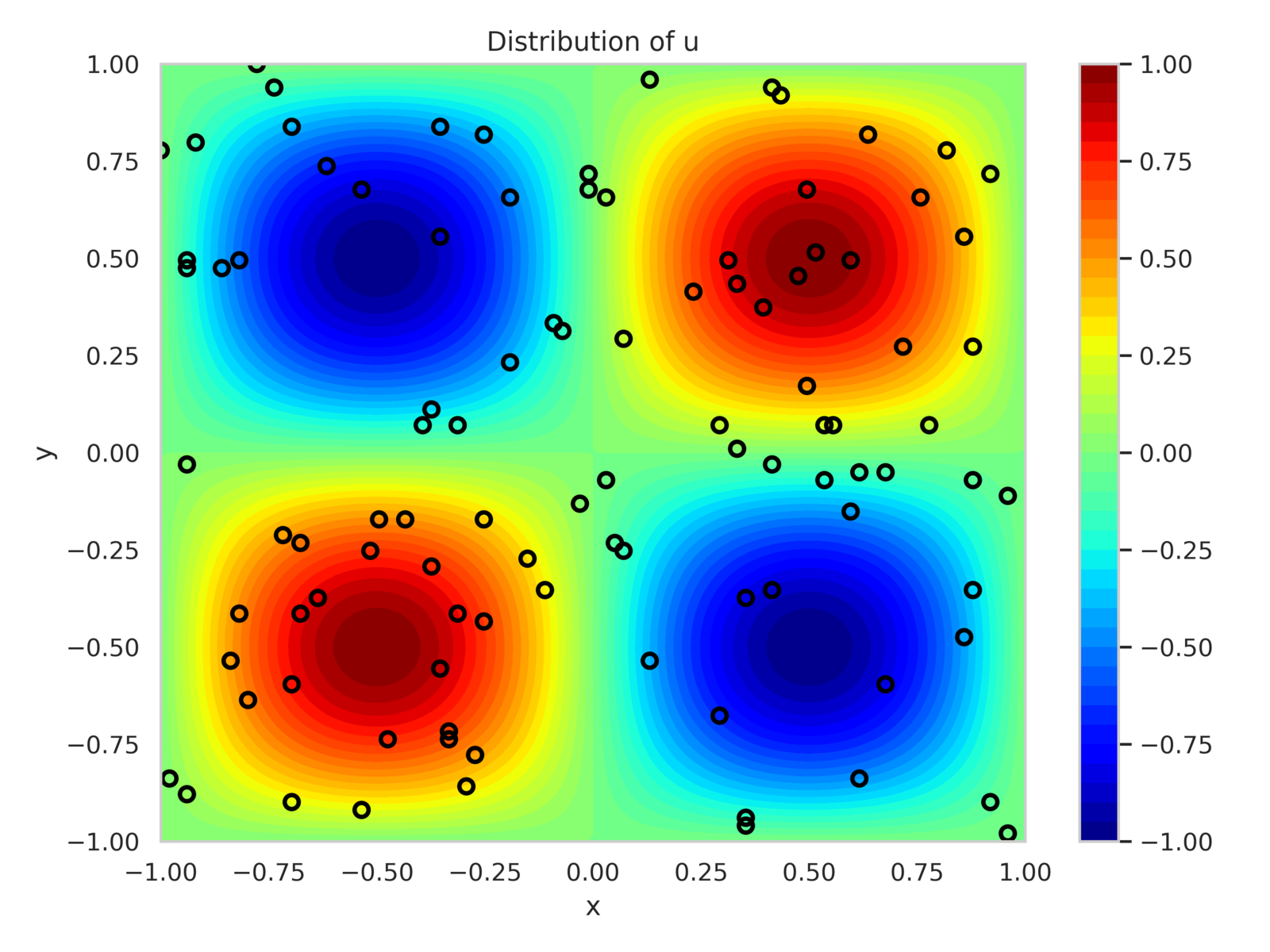
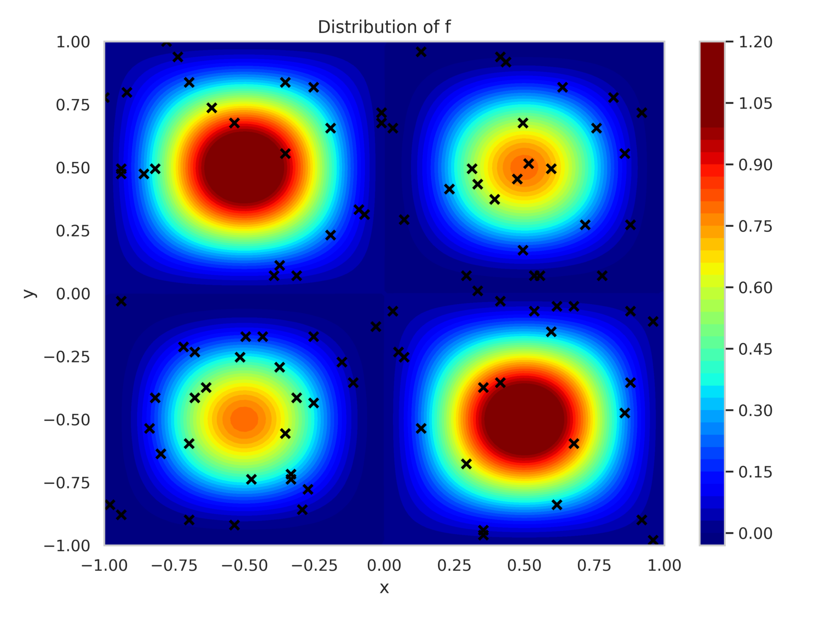
For and , the PDE has a known solution as given in eq. 19c. The training dataset consists of 100 randomly placed sensors within the domain that observe and , with added observation noise of variance . Additionally, 25 sensors are uniformly placed along each boundary to enforce Dirichlet boundary conditions.
Figure 8 shows the sensor positions along with contours of and . The model is configured with 300 neurons per hidden layer, totaling 272,703 trainable parameters. It is trained for 35,000 epochs using the Adam optimizer with a batch size of 500. Loss component weights are calibrated as:
This setup ensures the optimizer appropriately balances the various constraints.
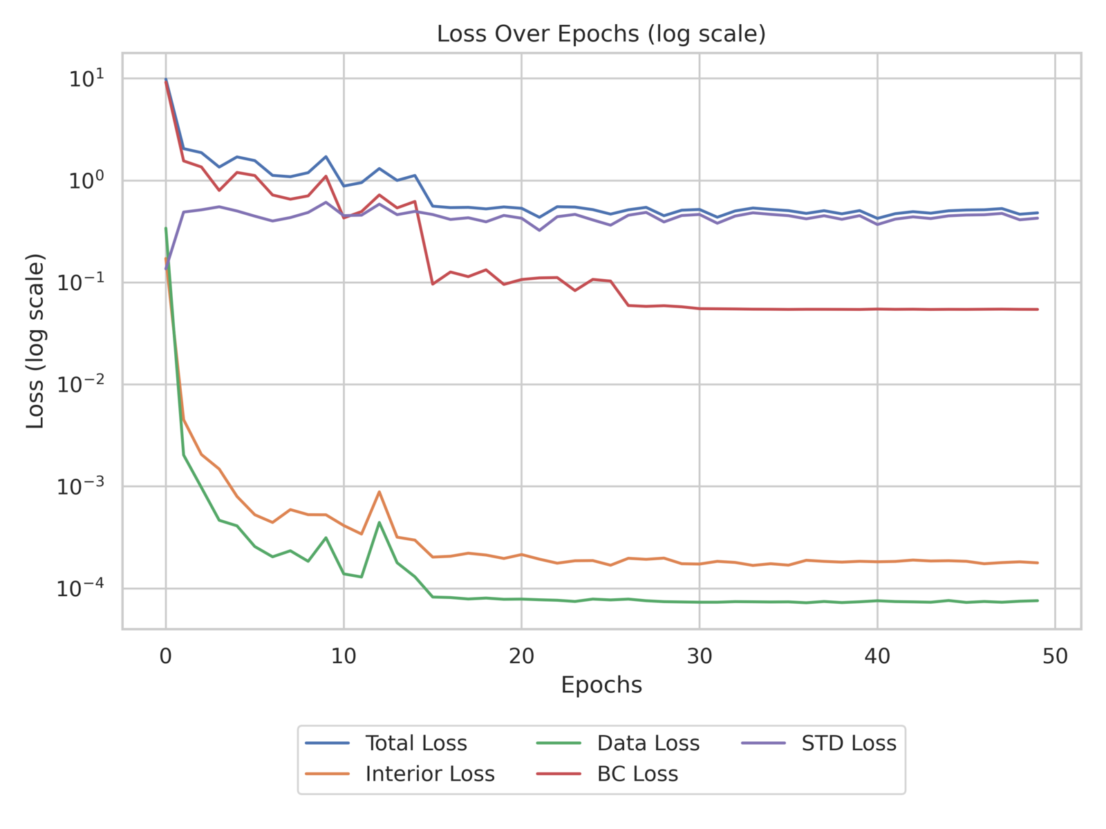
The training history, as shown in fig. 9, demonstrates consistent reduction in the PDE (Interior) and data losses during early epochs, followed by a decrease in the boundary condition loss. The variance of the posterior parameter distribution remains relatively unchanged due to the KL divergence term in the loss function.
Table 3 compares the estimated mean and standard deviation of the reaction rate using DeepBayONet and alternative Bayesian methods. DeepBayONet achieves results closest to the true value with the lowest standard deviation, demonstrating both accuracy and certainty in parameter estimation.
| DeepBayONet | B-PINN-HMC | B-PINN-VI | Dropout-1% | Dropout-5% | |
| Mean | 0.999 | 1.003 | 0.895 | 1.050 | 1.168 |
| Std |
We conducted a second experiment by relaxing boundary condition enforcement (). Figure 10 shows the residuals of the PDE when using the mean posterior parameter value. Higher residuals are observed at the boundaries when boundary conditions are excluded from training.
The posterior distributions of are shown in fig. 11. With boundary conditions, the posterior is narrow and centered around . Without boundary conditions, the posterior is wider, skewed, and exhibits a long tail, indicating increased uncertainty towards positive reaction rates.
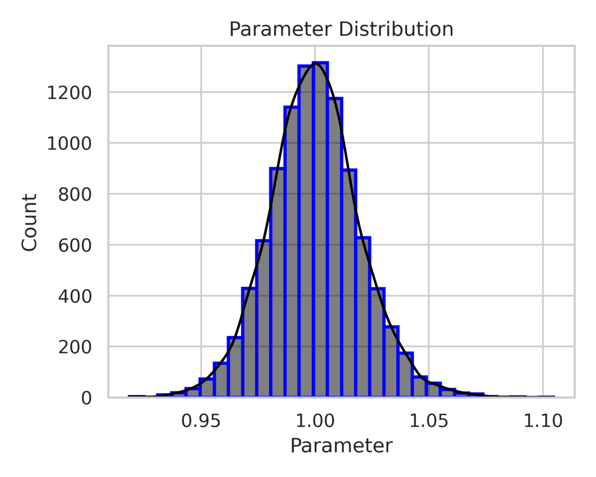
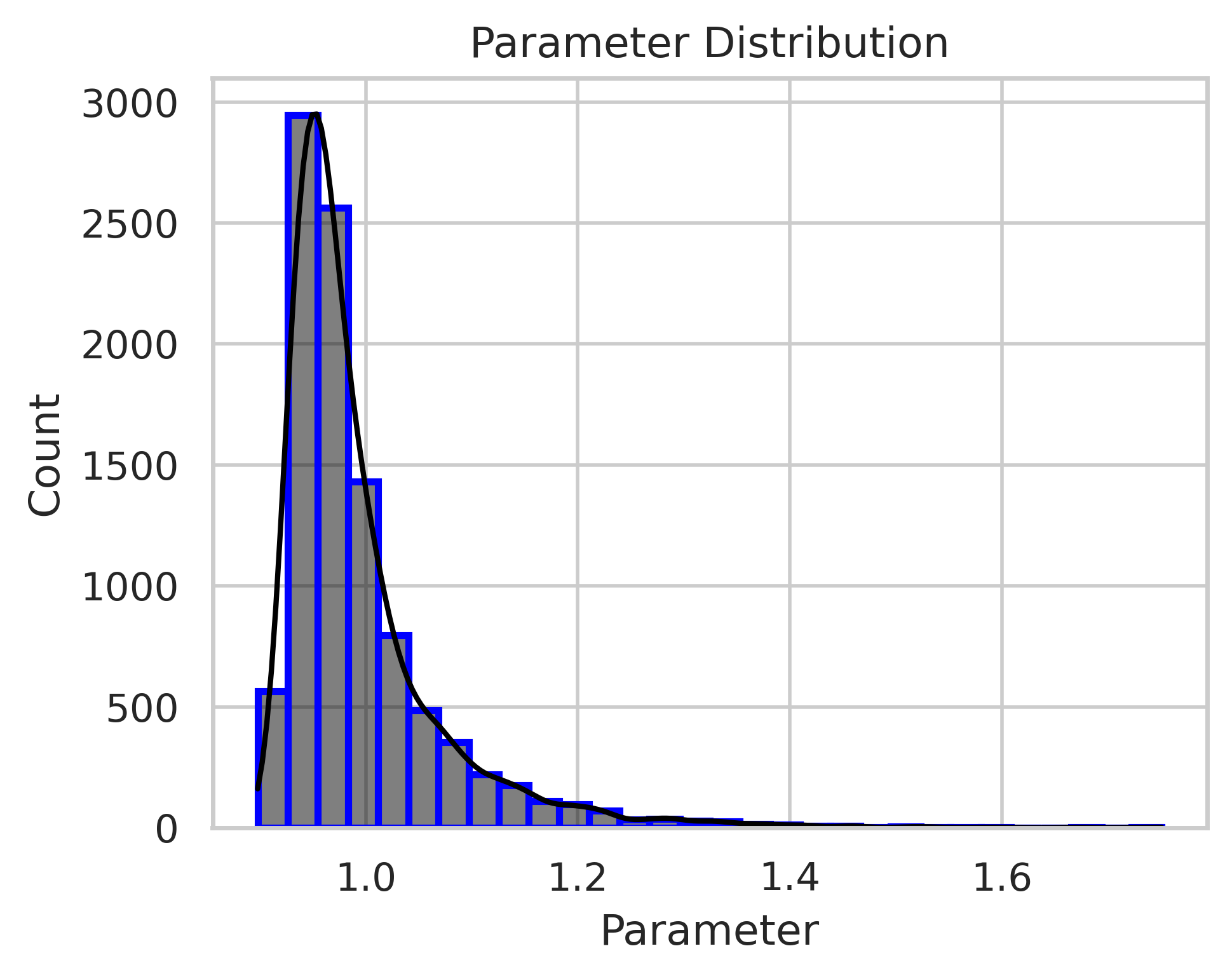
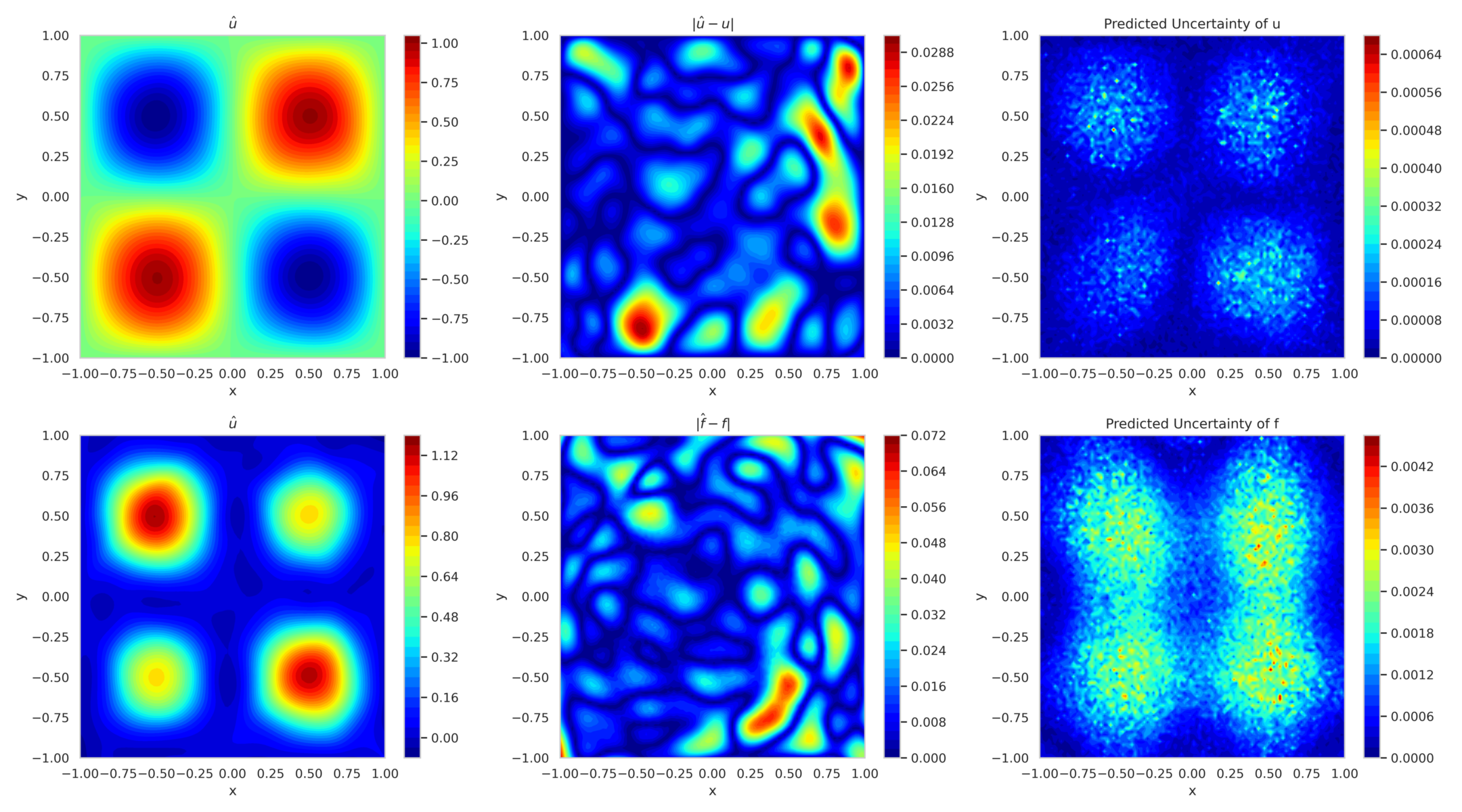
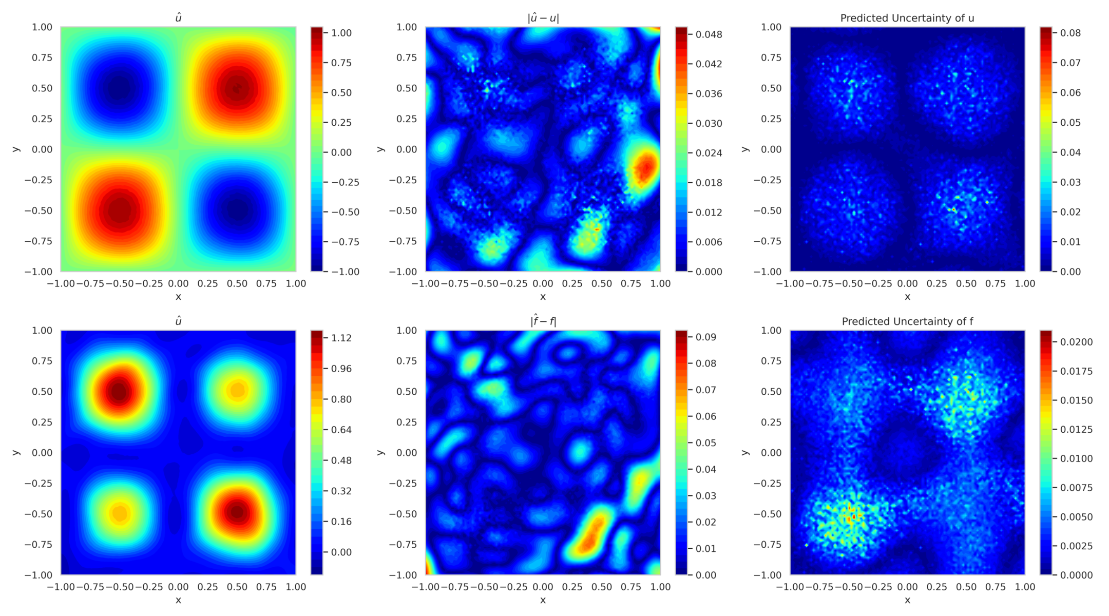
Figure 12 shows the mean predicted solution and its error along with the predicted uncertainty for boundary-enforced training. In fig. 13, the corresponding plots for boundary-free training reveal reduced accuracy and elevated uncertainty, highlighting the ability of model to adapt to missing boundary conditions.
4 Conclusions
This study introduces Bayesian Deep Operator Networks (DeepBayONet) integrated with Physics-Informed Neural Networks (PINNs) to address parameter estimation and uncertainty quantification challenges in solving partial differential equations (PDEs). By employing a Bayesian framework with variational inference, the approach effectively captures both epistemic and aleatoric uncertainties, offering robust predictions in noisy and data-scarce environments. The method demonstrates versatility across tasks, including forward and inverse problems in one- and two-dimensional PDEs, with a relatively low-cost computational efficiency on par with maximum likelihood training as opposed to the traditional Bayesian neural network training.
The framework provides several advantages. It achieves comprehensive uncertainty quantification, enabling reliable predictions under complex scenarios, and maintains competitive accuracy. Additionally, the architecture integrates seamlessly with modern deep learning frameworks, allowing for scalability in addressing high-dimensional and nonlinear challenges.
However, the method has limitations. It requires careful tuning of hyperparameters, such as weights for loss components, which can introduce manual overhead. Although more efficient than many Bayesian alternatives, variational inference remains computationally intensive compared to deterministic methods.
Future work could address these challenges by exploring adaptive strategies for loss weighting to improve usability and generalizability. Further refinement of prior distributions to incorporate domain-specific knowledge could enhance parameter estimation and uncertainty quantification. We have focused on Gaussian priors in this work. Expanding the approach to complex parameter distributions and multiscale and multiphysics systems can broaden its applicability.
Acknowledgements
This research was supported by the CSML lab and the College of Engineering at California State University Long Beach. The work used Jetstream2 at Indiana University through allocation CIS230277 from the Advanced Cyberinfrastructure Coordination Ecosystem: Services & Support (ACCESS) program, which is supported by National Science Foundation grants #2138259, #2138286, #2138307, #2137603, and #2138296.
References
- [1] S. Roberts, A. A. Popov, A. Sarshar, A. Sandu, A fast time-stepping strategy for dynamical systems equipped with a surrogate model, SIAM Journal on Scientific Computing 44 (3) (2022) A1405–A1427. doi:10.1137/20M1386281.
- [2] A. Sarshar, P. Tranquilli, B. Pickering, A. McCall, C. J. Roy, A. Sandu, A numerical investigation of matrix-free implicit time-stepping methods for large CFD simulations, Computers & Fluids 159 (2017) 53–63. doi:10.1016/j.compfluid.2017.09.014.
- [3] Y. Chen, Y. Shi, B. Zhang, Optimal Control Via Neural Networks: A Convex Approach (2019). doi:10.48550/arxiv.1805.11835.
- [4] R. Hwang, J. Y. Lee, J. Y. Shin, H. J. Hwang, Solving PDE-constrained Control Problems using Operator Learning (2021). doi:10.48550/arxiv.2111.04941.
- [5] S. Wang, M. A. Bhouri, P. Perdikaris, Fast PDE-constrained optimization via self-supervised operator learning, CoRR abs/2110.13297 (2021). doi:10.48550/arxiv.2110.13297.
- [6] A. Bhattacharjee, A. A. Popov, A. Sarshar, A. Sandu, Improving adam through an implicit-explicit (imex) time-stepping approach, Journal of Machine Learning for Modeling and Computing 5 (3) (2024). doi:10.1615/jmachlearnmodelcomput.2024053508.
- [7] M. Raissi, P. Perdikaris, G. E. Karniadakis, Physics-informed neural networks: A deep learning framework for solving forward and inverse problems involving nonlinear partial differential equations, Journal of Computational Physics 378 (2019) 686–707. doi:10.1016/j.jcp.2018.10.045.
- [8] L. Lu, X. Meng, Z. Mao, G. Karniadakis, DeepXDE: A deep learning library for solving differential equations, SIAM Review 63 (1) (2021) 208–228. doi:10.1137/19M1274067.
- [9] S. Cuomo, V. S. Di Cola, F. Giampaolo, G. Rozza, M. Raissi, F. Piccialli, Scientific machine learning through physics–informed neural networks: Where we are and what’s next, Journal of Scientific Computing 92 (3) (2022) 88. doi:10.1007/s10915-022-01939-z.
- [10] Z. Mao, A. D. Jagtap, G. E. Karniadakis, Physics-informed neural networks for high-speed flows, Computer Methods in Applied Mechanics and Engineering 360 (2020) 112789. doi:10.1016/j.cma.2019.112789.
- [11] G. Pang, L. Lu, G. E. Karniadakis, fPINNs: Fractional Physics-Informed Neural Networks, SIAM Journal on Scientific Computing 41 (4) (2019) A2603–A2626. doi:10.1137/18m1229845.
- [12] Y. Chen, L. Lu, G. E. Karniadakis, L. Dal Negro, Physics-informed neural networks for inverse problems in nano-optics and metamaterials, Optics Express 28 (8) (2020) 11618. doi:10.1364/oe.384875.
- [13] Q. He, D. Barajas-Solano, G. Tartakovsky, A. M. Tartakovsky, Physics-informed neural networks for multiphysics data assimilation with application to subsurface transport, Advances in Water Resources 141 (2020) 103610. doi:10.1016/j.advwatres.2020.103610.
- [14] E. A. Antonelo, E. Camponogara, L. O. Seman, E. R. de Souza, J. P. Jordanou, J. F. Hubner, Physics-Informed Neural Nets for Control of Dynamical Systems (2021). doi:10.48550/arxiv.2104.02556.
- [15] J. Barry-Straume, A. Sarshar, A. A. Popov, A. Sandu, Physics-informed neural networks for pde-constrained optimization and control, arXiv preprint (2022). doi:10.48550/arXiv.2205.03377.
- [16] R. Nellikkath, S. Chatzivasileiadis, Physics-Informed Neural Networks for Minimising Worst-Case Violations in DC Optimal Power Flow (2021). doi:10.48550/arxiv.2107.00465.
- [17] D. Zhang, L. Lu, L. Guo, G. E. Karniadakis, Quantifying total uncertainty in physics-informed neural networks for solving forward and inverse stochastic problems, Journal of Computational Physics 397 (2019) 108850. doi:10.1016/j.jcp.2019.07.048.
-
[18]
A. Paszke, S. Gross, S. Chintala, G. Chanan, E. Yang, Z. DeVito, Z. Lin,
A. Desmaison, L. Antiga, A. Lerer,
Automatic differentiation in
PyTorch (Oct. 2017).
URL https://openreview.net/forum?id=BJJsrmfCZ -
[19]
J. Bradbury, R. Frostig, P. Hawkins, M. J. Johnson, C. Leary, D. Maclaurin,
S. Wanderman-Milne, JAX: composable
transformations of Python+NumPy programs, version 0.2.26 (2018).
URL http://github.com/google/jax -
[20]
M. Abadi, et al., Tensorflow: Large-scale
machine learning on heterogeneous systems, software available from
tensorflow.org (2015).
URL https://www.tensorflow.org/ - [21] A. G. Baydin, B. A. Pearlmutter, A. A. Radul, J. M. Siskind, Automatic differentiation in machine learning: A survey, Journal of Machine Learning Research 18 (153) (2018) 1–43. doi:10.5555/3327757.3327758.
- [22] C. C. Margossian, A review of automatic differentiation and its efficient implementation, WIREs Data Mining and Knowledge Discovery 9 (4) (2019) e1305. doi:10.1002/widm.1305.
- [23] F. A. C. Viana, A. K. Subramaniyan, A survey of bayesian calibration and physics-informed neural networks in scientific modeling, Archives of Computational Methods in Engineering 28 (5) (2021) 3801–3830. doi:10.1007/s11831-021-09539-0.
- [24] J. P. Molnar, S. J. Grauer, Flow field tomography with uncertainty quantification using a Bayesian physics-informed neural network, Measurement Science and Technology 33 (6) (2022) 065305, publisher: IOP Publishing. doi:10.1088/1361-6501/ac5437.
- [25] Y. Li, Y. Wang, L. Yan, Surrogate modeling for Bayesian inverse problems based on physics-informed neural networks, Journal of Computational Physics 475 (2023) 111841. doi:10.1016/j.jcp.2022.111841.
- [26] H. Wang, D.-Y. Yeung, A survey on bayesian deep learning, ACM Computing Surveys 53 (5) (2020) 108:1–108:37. doi:10.1145/3409383.
- [27] C. Bonneville, C. Earls, Bayesian deep learning for partial differential equation parameter discovery with sparse and noisy data, Journal of Computational Physics: X 16 (2022) 100115. doi:10.1016/j.jcpx.2022.100115.
- [28] P. Izmailov, S. Vikram, M. D. Hoffman, A. G. G. Wilson, What are bayesian neural network posteriors really like?, Proceedings of the 38th International Conference on Machine Learning 139 (2021) 4629–4640. doi:10.48550/arXiv.2104.14421.
- [29] L. Yang, X. Meng, G. E. Karniadakis, B-PINNs: Bayesian physics-informed neural networks for forward and inverse PDE problems with noisy data, Journal of Computational Physics 425 (Jan. 2021). doi:10.1016/j.jcp.2020.109913.
- [30] T. Chen, H. Chen, Universal approximation to nonlinear operators by neural networks with arbitrary activation functions and its application to dynamical systems, IEEE Transactions on Neural Networks 6 (4) (1995) 911–917. doi:10.1109/72.392253.
- [31] L. Lu, P. Jin, G. E. Karniadakis, Deeponet: Learning nonlinear operators for identifying differential equations based on the universal approximation theorem of operators, arXiv preprint (2019). doi:10.48550/arXiv.1910.03193.
- [32] A. Kendall, Y. Gal, What Uncertainties Do We Need in Bayesian Deep Learning for Computer Vision?, in: Advances in Neural Information Processing Systems, Vol. 30, Curran Associates, Inc., 2017. doi:10.5555/3295222.3295309.
- [33] N. Srivastava, G. Hinton, A. Krizhevsky, I. Sutskever, R. Salakhutdinov, Dropout: A simple way to prevent neural networks from overfitting, Journal of Machine Learning Research 15 (1) (2014) 1929–1958.
- [34] Z. Xiang, W. Peng, X. Liu, W. Yao, Self-adaptive loss balanced physics-informed neural networks, Neurocomputing 496 (2022) 11–34. doi:10.1016/j.neucom.2022.05.015.
- [35] L. D. McClenny, U. M. Braga-Neto, Self-adaptive physics-informed neural networks, Journal of Computational Physics 474 (2023) 111722. doi:10.1016/j.jcp.2022.111722.
-
[36]
DeepFindr, How to handle
uncertainty in deep learning, [Online; accessed 2024-12-26].
URL https://www.youtube.com/watch?v=WWATIH5ZACw - [37] M. Abdar, F. Pourpanah, S. Hussain, D. Rezazadegan, L. Liu, M. Ghavamzadeh, P. Fieguth, X. Cao, A. Khosravi, U. R. Acharya, et al., A review of uncertainty quantification in deep learning: Techniques, applications and challenges, Information fusion 76 (2021) 243–297. doi:10.1016/j.inffus.2021.05.008.