Deep model simulation of polar vortices in gas giant atmospheres
Abstract
The Cassini and Juno probes have revealed large coherent cyclonic vortices in the polar regions of Saturn and Jupiter, a dramatic contrast from the east-west banded jet structure seen at lower latitudes. Debate has centered on whether the jets are shallow, or extend to greater depths in the planetary envelope. Recent experiments and observations have demonstrated the relevance of deep convection models to a successful explanation of jet structure, and cyclonic coherent vortices away from the polar regions have been simulated recently including an additional stratified shallow layer. Here we present new convective models able to produce long-lived polar vortices. Using simulation parameters relevant for giant planet atmospheres we find flow regimes of geostrophic turbulence (GT) in agreement with rotating convection theory. The formation of large scale coherent structures occurs via three-dimensional upscale energy transfers. Our simulations generate polar characteristics qualitatively similar to those seen by Juno and Cassini: they match the structure of cyclonic vortices seen on Jupiter; or can account for the existence of a strong polar vortex extending downwards to lower latitudes with a marked spiral morphology, and the hexagonal pattern seen on Saturn. Our findings indicate that these vortices can be generated deep in the planetary interior. A transition differentiating these two polar flows regimes is described, interpreted in terms of force balances and compared with shallow atmospheric models characterising polar vortex dynamics in giant planets. In addition, heat transport properties are investigated, confirming recent scaling laws obtained with reduced models of GT.
keywords:
thermal rotating convection – geostrophic turbulence – polar dynamics – gas giant atmospheres1 Introduction
Zonal (east/west directed) wind circulations are ubiquitous in gas giant planets. Jupiter and Saturn have strong prograde (eastward) equatorial jets that extend into the deep interior molecular envelope (Kaspi et al., 2018; Guillot et al., 2018). In addition, coherent vortices and related structures are found to be very robust close to polar latitudes (Adriani et al., 2018; Fletcher et al., 2018). Current modelling of gas giant flow dynamics involves two different approaches (Showman et al., 2018): a shallow-layer scenario in which baroclinic turbulence is feeding the jets in a thin atmospherical layer (Liu & Schneider, 2010; Morales-Juberías et al., 2015; Rostami et al., 2017); or a deep scenario (Busse, 1976; Heimpel et al., 2005; Heimpel & Aurnou, 2007; Heimpel et al., 2015) in which the jets form quasigeotrophic columns extending down into the molecular envelope. Which approach is best is still under debate but recent laboratory experiments (Cabanes et al., 2017), reproducing jet properties at high latitudes in the presence of viscous damping, recent observations of the deep extension of the Jovian jet streams (Kaspi et al., 2018), and analysis of Cassini data from two different pressure levels within Saturn’s polar winds (Studwell et al., 2018) all favour the deep approach.
Three-dimensional deep models of the molecular envelope in a rotating spherical geometry (Heimpel et al., 2005; Heimpel & Aurnou, 2007) have provided a strong background for understanding the mechanisms of jet formation, in which geostrophic turbulence (GT) is a key issue (Rhines, 1975). The deep convection models of Heimpel & Aurnou (2007) interpreted the transition between Jupiter and Saturn’s flow regimes by considering different spherical shell widths, pointing out the relevance of the tangent cylinder (a coaxial cylinder touching the inner boundary at the equator) on the equatorial jet width. The existence of such an internal boundary for zonal jets has been one of the main concerns for deep modelling (Showman et al., 2018), but recent gravity field measurements by the Juno mission (Guillot et al., 2018) have confirmed that zonal jets extend deeper into Jupiter’s atmosphere. The current explanation for this internal boundary involves the existence of magnetic field drag acting on the flow (Liu et al., 2008). Measurements of the electrical conductivity in the molecular envelope were used to constrain the extent of zonal jets, giving a lower boundary for Jupiter and Saturn estimated to be 0.96R and 0.86R (R being the planetary radius), respectively (Liu et al., 2008), which match quite well with those obtained with recent gravity measurements (Guillot et al., 2018).
Polar coherent vortices in Jupiter were discovered very recently (Adriani et al., 2018) and thus much of the modelling of polar vortices to date has focused on Saturn. Observations have revealed a seasonal influence on the morphology of polar flow structure (Sayanagi et al., 2017; Fletcher et al., 2018) involving a strong single polar vortex with associated spiralling arms. A hexagonal structure is present near north latitude at stratospherical levels, which was believed to be the result of a Rossby wave trapped in the troposphere (Godfrey, 1988; Fletcher et al., 2018). Existing models of Saturn’s hexagonal pattern and polar vortices assume shallow jet structures (Morales-Juberías et al., 2015; Rostami et al., 2017) and can explain key features of the hexagonal pattern such as its latitudinal location, almost steady azimuthal drift and the absence of large vortices close to the structure. However, there is debate about whether this hexagonal jet has a deep origin, as the long term observations from the Cassini mission suggest (Baines et al., 2009; Sánchez-Lavega et al., 2014). In the case of Jupiter, the first close-up images of north pole revealed the coexistence of cyclonic vortices, oval-shaped structures, filamentary regions and thin linear features elongated more than in the azimuthal direction, concentrated from latitude polewards (Orton et al., 2017). Subsequent Juno data analysis confirmed the persistence of these flow structures: 8 vortices surround the main cyclonic north polar vortex, whereas only 5 vortices are found surrounding the main cyclonic south polar vortex (Adriani et al., 2018).
Direct numerical simulations (DNS) of shallow atmospheric models (Scott, 2011; O’Neill et al., 2015, 2016) have been used to understand polar atmospheric dynamics of giant planets (see the comprehensive review of Sayanagi et al. 2018 in the case of Saturn), especially the case of polar cyclones. The latter studies consider a source term which accounts for small-scale features produced by moist convective storms (O’Neill et al., 2015, 2016) and drives turbulence. The idea behind this approach is that cyclonic vortices form as a result of poleward flux of cyclonic vorticity caused by the beta-drift, i.e. the advection of the background potential vorticity by the storm circulation. The moist baroclinic forcing is then responsible for the generation of a barotropic vortex aligned in the vertical direction (O’Neill et al., 2015). This study first demonstrated that the vortex features of the flow, i. e. the appearance (or not) of a single vortex centered at the poles, is controlled by the ratio of two characteristic sizes, namely, that of the small vortices and the planetary radius. The recent study by Brueshaber et al. (2019) provides further support for the mechanism which distinguishes the specific characteristics of polar dynamics occurring in Jupiter (a ring of cyclones surrounding the poles) and Saturn (single and strong cyclone) studied in O’Neill et al. (2015, 2016). The key parameter which controls the transition between the latter scenarios is the Burger number, defined as the ratio between the Rossby deformation radius and the planetary radius (Brueshaber et al., 2019). As the Burger number is decreased a transition from Saturn-like to Jupiter-like polar cyclones is observed.
Rotating Rayleigh-Bénard convection between plane boundaries constitutes a reasonable approximation for studying polar dynamics in gas giant atmospheres as the convective region is very thin when compared to the planetary radius. Within this canonical framework much theoretical and numerical work has recently been done by Julien et al. (2012a, b); Rubio et al. (2014) to investigate the regime of GT in terms of a 3D reduced model including boundary effects. The latter studies identified the physical mechanisms involved in the formation of large-scale coherent structures surrounding the rotation axis as a result of a fully three-dimensional convective forcing (Rubio et al., 2014). The associated efficient mixing within the fluid reduces the heat transport and determines its scaling law (Julien et al., 2012b). According to Julien et al. (2012a) the realisation of the GT regime, in which the flow is weakly dependent on the axial coordinate, depends strongly on the input parameters, particularly the Prandtl number associated with the thermal properties of the fluid. For smaller Prandtl numbers the GT regime is favoured, in agreement with our results.
The formation of these coherent structures at polar latitudes in giant planets remains to be reproduced within the context of deep convection modelling. This is the focus of the present study, based on three dimensional DNS of Boussinesq thermal convection in rotating spherical shells without any symmetry assumption. In Sec. 2 the model equations, numerical method and the physical parameters of the models are described. Sec. 3 constitutes the main part of the study. It includes the description of the flow patterns and their time averaged properties, the investigation of a condensate process and the transition between polar regimes, the study of the force balance and the thermal properties, and the characterisation of a Saturn-like hexagonal pattern. Finally, a summary of the main results and future investigations is provided in Sec. 4. In this closing section, we also include a discussion of the validity of the approximations and approaches taken, when applying our findings to the giant planets.
2 The model
2.1 Governing equations and numerical method
A homogeneous fluid with density and constant physical properties –thermal diffusivity , thermal expansion coefficient , and dynamic viscosity – is considered, to study thermal convection in a rotating spherical shell. The latter is defined by the inner and outer radius and , and a constant angular velocity about the vertical axis. Gravity acts in the radial direction ( is constant and the position vector) and the relation is assumed (the Boussinesq approximation), but just in the gravitational term. For the other terms appearing in the equations a reference state is considered (see for instance Pedlosky 1979; Chandrasekhar 1981).
At the boundaries, which are perfectly conducting, a temperature difference is imposed , and . Stress-free boundary conditions for the velocity field are appropriate for planetary atmospheres (Christensen, 2002; Heimpel et al., 2005). The mass, momentum and energy equations are written in the rotating frame of reference as in Simitev & Busse (2003) and expressed in terms of velocity () and temperature () perturbations of the basic conductive state and , being the aspect ratio, being the gap width, and being a reference temperature. With units for the distance, for the temperature, and for the time, the governing equations read
| (1) | |||
| (2) | |||
| (3) |
being is a dimensionless scalar containing all the potential forces. Centrifugal effects are neglected by assuming . This is usual for the case of spherical shell convection (Schubert & Zhang, 2000). Four non-dimensional parameters -the aspect ratio , the Rayleigh , Prandtl , and Taylor numbers- summarise the physics of the problem. The Prandtl number characterises the relative importance of viscous (momentum) diffusivity to thermal diffusivity, the Taylor number is the ratio between rotational and viscous forces, and the Rayleigh number is associated with buoyancy forces and thermal forcing. The parameters are defined by
| (4) |
To solve the model equations 1-3 with the prescribed boundary conditions a pseudo-spectral method (Tilgner, 1999) is used (see Garcia et al. 2010 for a detailed description). In the radial direction a collocation method on a Gauss–Lobatto mesh (Sánchez et al., 2016) is considered and spherical harmonics are employed in the angular coordinates. In the Boussinesq approximation the toroidal/poloidal decomposition for the velocity field can be used (Chandrasekhar, 1981). The code is parallelized in the spectral and in the physical space using OpenMP directives. Optimized libraries (FFTW3, Frigo & Johnson, 2005) for the fast Fourier transforms FFTs in longitude and matrix-matrix products (dgemm GOTO, Goto & van de Geijn, 2008) for the Legendre transforms in latitude are implemented for the computation of the nonlinear terms. Aliasing is properly removed in the pseudo-spectral transform method (Orszag, 1970).
High order implicit-explicit backward differentiation formulas (IMEX–BDF, Garcia et al., 2010) are used for the time integration of the discretized equations. The nonlinear terms are considered explicitly, to avoid solving nonlinear equations at each time step. However, the Coriolis term is treated fully implicitly and this allows a time integration with larger time steps (Garcia et al., 2010).
2.2 Model parameters
| Model | 1 | 2 |
|---|---|---|

Two different models of Boussinesq thermal convection are considered to explore the transition from Saturn-like (Model 1) to Jupiter-like (Model 2) polar dynamics. In these two models the parameters , and are the same. They are similar to previous numerical models of gas giant atmospheres (Heimpel et al., 2005; Heimpel & Aurnou, 2007; Heimpel et al., 2015) focusing on the understanding of jet dynamics away from the polar regions. We select an aspect ratio which roughly falls between the values estimated for Jupiter and Saturn (Liu et al., 2008). We set a sufficiently large Taylor number, - as used in Heimpel et al. (2005); Heimpel & Aurnou (2007); Heimpel et al. (2015) - and a Prandtl number , which is a reasonable regime for gas giant atmospheres (French et al., 2012) due the uncertainty in determining . A key difference between the current polar models and those of Heimpel et al. (2005); Heimpel & Aurnou (2007) and Heimpel et al. (2015) devoted to lower latitudes, is the selection of a small Prandtl number, which strongly influences the type of convection (Simitev & Busse, 2003; Kaplan et al., 2017; Garcia et al., 2019). In our case convection directly onsets at high latitudes (Garcia et al., 2018) whereas previous deep models require a strong nonlinear regime to develop polar convection.
With an aspect ratio of , and convective onset takes the form of nonaxisymmetric polar modes confined to large latitudes (Garcia et al., 2008, 2018) at a critical Rayleigh number . The main difference between our two models comes from the Rayleigh number. Model 1 (M1) corresponds to (), whereas Model 2 (M2) corresponds to a slightly larger (). For low Prandtl and large Taylor numbers even a small degree of supercriticallity provides strong turbulent flows (Kaplan et al., 2017), characterised by a predominance of advection, rather than diffusion, in the temperature transport.
The DNS presented here have spatial resolutions very similar to those used in previous deep convection models for the same range of parameters (Eg. Heimpel et al. 2005, 2015). Specifically, we consider spherical harmonics up to order and degree and a radial mesh with points. In contrast to previous studies, however, our numerical simulations do not rely on the use of azimuthal symmetry constraints, nor on imposed hyperviscosity, allowing us to capture low wave number coherent dynamics in the flow. These are otherwise filtered if -fold symmetry constraints are imposed. However, the system of equations has in return dimension , making the numerical integration of Models 1 and 2 very challenging.
Both models are evolved for around one viscous time unit ( for M1 and for M2), including a large initial transient, with a time step of . The initial condition for integrating Model 1 corresponds to a transient flow at the same and but with . The latter simulation has been initialised from a model at , , and () obtained from the chaotic polar flows described in Garcia et al. (2019). Model M2, with larger , is obtained from M1. This is a common strategy in deep convection models (Christensen, 2002; Heimpel et al., 2005; Garcia et al., 2014). Because of the large dimension of the system (which has been integrated without any symmetry assumption) and the small time step required to obtain the numerical simulations, only two simulations are presented. These are however some of the highest resolution convective models, in rotating thin shells, performed to date.
The two models exhibit features of turbulent flows that occur in gas giant atmospheres. The values shown in Table 1 of the time and volume averaged Rossby (measuring the balance between Coriolis and inertial forces) or Reynolds (a measure of turbulent flows) numbers are in agreement with those given in previous studies on gas giant atmospheres, for instance those based on the peak zonal flow velocities, given in Table II of Heimpel & Aurnou (2007). The modified Rayleigh number , measuring the ratio of buoyancy to Coriolis forces, matches reasonably as well. In addition, the Péclet number (measuring the ratio of temperature transport by advection and diffusion) is larger than (see Kaplan et al. 2017) a value which marked the transition between laminar and turbulent flows at low and large .
3 Deep polar flow dynamics
In this section we explore and analyse in detail the new regime of polar convection exhibited by our two models, M1 and M2, focusing on its relation to the polar dynamics observed on Saturn and Jupiter. First, we provide a description of the main characteristics of the flow patterns, followed by an analysis of time averaged flow latitude profiles. Second, we identify a turbulent energy transfer mechanism by means of kinetic energy spectra, which in turn are compared with results from the Cassini mission. Third, the appearance of different coherent polar structures is interpreted within recent theoretical results of 3D rotating convection, and related to shallow water models of Saturn and Jupiter. We then analyse the force balance and the properties of thermal transport. This section closes with the description of a Saturn-like hexagonal flow pattern, surrounding the north pole, observed in M1.
3.1 Description of flow patterns


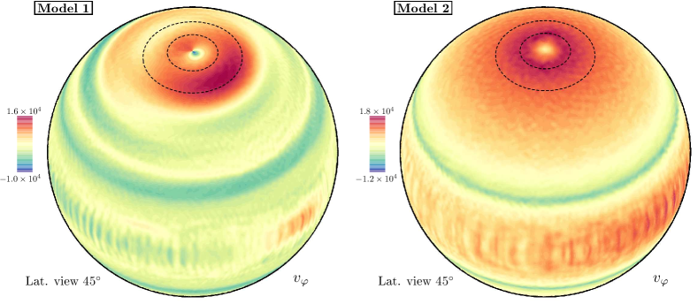
Figure 1 displays snapshots of the contour plots of the azimuthal velocity at the outer sphere and the radial velocity at the sphere with radius (i.e. in the middle of the shell) for both models. The spheres are viewed from latitude, and the and parallels surrounding the north pole are marked with a dashed line. The flow is strongly axisymmetric for both models (see first row of Fig. 1) as is typical in stress-free convection models (Aurnou & Olson, 2001; Christensen, 2002), with a noticeable wide positive (prograde) equatorial band which is more evident for M2. This is typical for flows with (Eg. Aurnou et al. 2007) in which the Coriolis forces dominate over buoyancy effects. In this case Reynolds stresses associated with columnar convection are feeding the zonal flow at mid and low latitudes (Christensen, 2002). In contrast to the latter studies, strong prograde zonal flows are produced at high latitudes in models M1 and M2.
The main difference between the models is in the latitudinal extent of these high latitude zonal circulations and their topology, which for M1 has a noticeable azimuthal wave number component. The existence of small scale vortices associated with turbulent flows is best seen in the contour plots of the radial velocity (second row of Fig. 1). In this case very small scale flow structures at high latitudes coexist with large scale cells elongated in the axial direction near the equator. As evidenced by the figure, the radial vortices within the parallel are stronger in the case of M2. The geostrophic character of the flows, i.e. the tendency of the flow to align with the rotation axis, is reflected in Figure 2 on the meridional sections of and . The zonal circulation of polar jets extends down to the inner boundary and is almost independent of the coordinate. This is fulfilled for the small as well as the large scale radial vortices. Notice how these large scale cells are only allowed to grow outside the tangent cylinder.

Figure 3 shows the radial vorticity patterns on the outer sphere for M1 and M2. This figure displays a transition, in agreement with shallow layer models O’Neill et al. (2015, 2016); Brueshaber et al. (2019), in which a single polar vortex (M1) is divided into smaller vortices (M2) as the thermal forcing () is increased. The flow structure of M1, seen in the first row of Fig. 3, reveals key features similar to those that appear in Saturn’s atmosphere (Cassini mission, Sayanagi et al., 2017). There is a single strong cyclonic vortex almost centered at both poles and with spiralling morphology. The polar vortices are surrounded by circular belts containing small vortices far away from latitude. These two strong cyclones are present throughout the simulation (at least one viscous time unit) in agreement with the observations (Fletcher et al., 2015).
In contrast to M1, the DNS corresponding to M2 (2nd row of Fig. 3) has long-lived polar structures resembling the polar features observed in Jupiter’s atmosphere (Adriani et al., 2018). It reveals the prevalence of several strong cyclonic coherent vortices close to the north as well as south pole, some of them with an oval shape. Azimuthally elongated structures exist, in agreement with the observations of the Juno mission (Orton et al., 2017; Adriani et al., 2018). In addition, far away from the polar regions, circular vortices are arranged in parallel lines (east-west) and the strongest lie very close to latitude, in either the northern or southern hemisphere as previously simulated in Heimpel et al. (2015) with stratified convection models.
We note that Figure 3 evidences a multimodal structure as found in the rotating convection experiments of Aurnou et al. (2018) at similar number. Modes with are responsible for long lived polar vortices, which extend down to the inner boundary, as well as low latitude large-scale cells (meridional sections of Fig. 2). In contrast, high wave numbers only contribute far away from the latitude circles . For this component of the flow two different sizes of vortex are observed: those elongated in the latitudinal direction near equatorial latitudes and those with oval shape appearing around latitudes.
3.2 Time averaged latitude profiles
The latitude profiles at the outer surface shown in Fig. 4 mark the latitude position of the key features for both models seen in the previous figures. The time averaged Rossby number (ratio of inertial to Coriolis forces) and radial vorticity are plotted versus latitude for both models. The time series span a interval of around 1300 planetary rotations for Model 1 and 1500 for Model 2, with a time step of around 20 planetary rotations in both models. The time averaged zonal Rossby number (where is the azimuthal average of the azimuthal velocity) is not displayed since it is almost equal to the time averaged , i.e. nonaxisymmetric time fluctuations tend to cancel out. For both models the Rossby number is clearly large close to the poles (see Fig. 4, panels (a,c)) and remains smaller at equatorial latitudes. This means that our modelling is not reasonable for the study of dynamical behaviour of gas giant planets at low latitudes (Heimpel & Aurnou, 2007; Heimpel et al., 2005, 2015), although it reproduces qualitatively several key features of the equatorial wind such as its latitudinal extent, the negative peaks close to latitudes and even a noticeable decrease of magnitude near the equator (see Fig. 4(c)). The polar dynamics exhibited by the present models is a new feature not previously observed in rotating thermal convection in spherical shells. There are two peaks of around and for Model 1 and they are located closer to the poles and for Model 2. Indeed, the time dependence away from latitudes is significantly more vigorous for Model 1. For this model the maximum and minimum curves of clearly display two latitudes and for which remains roughly constant. Besides a transition between different polar vortex characteristics between Model 1 and 2, there is also a transition between equatorial behaviour: the time dependence of for Model 2 is enhanced near the equator ( latitudes) providing maximum values of around latitude, comparable to the peaks near the poles (see Fig. 4(c)).
The radial vorticity latitude profiles shown in Fig. 4(b,d) clearly display a strong time dependence of vorticity. The main characteristic featured by both models is the strong cyclonic vorticity near both poles. For Model 1 the polar jet extends down to latitudes (where becomes zero) and a similar extent, down to , is reached for Model 2. For the latter, the relative maximum/minimum near marks the position of the several circumpolar vortices. The radial vorticity of Model 2 exhibits stronger oscillations at lower latitudes, especially around , where the time average amplitude is noticeable. The relative extrema at intermediate latitudes are larger for Model 1, indicating that vortex activity is more vigorous (compare also the contour plots seen in Fig. 3). The bottom row of Fig. 4 evidences the different mode contribution to vortex activity in Model 2 by considering only the spherical harmonics with or with . The time averaged of the latter component is nearly zero, meaning that the main contribution to mean vorticity comes from low order modes. Indeed, the time dependent is zero near the poles for the component of the flow, and thus the latter does not contribute to the origin of the polar dynamics.
Quantitatively, our models underestimate the zonal wind amplitudes measured in gas giant planets. For instance, in the case of Saturn (Sayanagi et al., 2018) the peak zonal winds close to the poles (around latitude, Sánchez-Lavega et al. 2006) are around m/s giving rise to which is roughly three times that measured for Model 1. As commented previously, values for the parameters are not so far from those obtained from the DNS of Heimpel & Aurnou (2007); Heimpel et al. (2005, 2015) (at larger ) modelling wind jets at moderate and low latitudes. However, our models exhibit larger and circular vortices at high latitudes, in contrast to previous modelling. In addition, preliminary results for models with larger point to a decrease of zonal flows and a disappearance of coherent structures in the polar regions. Thus there exists a flow transition, in which zonal flow and vortices at high latitudes progressively weaken, in a parameter regime relevant for giant planetary atmospheres. This transition also occurs at lower rotation rates when polar modes are preferred at the onset (Garcia et al., 2019). Understanding this transition may provide a simple explanation for the existence of polar convective coherent vortices in planetary atmospheres.
3.3 Kinetic energy spectra and energy transfer mechanism

An analysis of the kinetic energy distribution among the spherical harmonic modes with different degree is performed, to elucidate the inverse cascade mechanism for these three-dimensional rapidly rotating flows (Rubio et al., 2014). In addition, kinetic energy spectra are a tool which helps to validate the spherical harmonic resolution of a given DNS. A rule of thumb (Christensen et al., 1999; Kutzner & Christensen, 2002) indicates that a model is well resolved if the kinetic energy decreases by more than two orders of magnitude from the maximum to the smallest wave-length scale.
Figure 5(a,b) displays the volume averaged kinetic energy (dashed line) and the surface averaged kinetic energy at (solid line) of a particular mode with degree for both models M1 and M2. Notice that the energies of few harmonics just before the maximum spectral degree increase a little bit. This behaviour is present in some three-dimensional DNS in rotating spherical geometry, but it has been shown (see Christensen et al. 1999 for the geodynamo case) that a reasonable energy increase at the tail does not significantly alter the large-scale structure of the flow.
The spectra exhibit slopes of and which are in reasonable agreement with those obtained from 2D maps of velocity measurements extracted from Cassini images (Choi & Showman, 2011). Furthermore, the distribution of energy among the different degree displayed in Fig. 5(a,c) resembles the distribution exhibited on Fig.5(a) of Choi & Showman (2011), constructed from Jovian velocity measurements. Because the flow has a strong equatorially symmetric component, odd have larger energy than even , especially for low values, giving rise to the spiking behaviour of the spectra. Note that Choi & Showman (2011) computes the power spectra of kinetic energy, rather than the energy content of each mode, so that even have larger energy. The length scale marking the change of slope from to of the Jovian spectra of Choi & Showman (2011), assumed to be the scale at which energy is injected to the system, is in the interval depending whether global or eddy kinetic energy are considered. In our case the situation is similar and the slope is lost from in the case of M1 or from in the case of M2.
In the context of three-dimensional Rayleigh-Bénard rotating convection an upscale energy transfer mechanism, known as the condensation process, has recently been identified in the regime of GT (Rubio et al., 2014). Large scale barotropic vortices, fulfilling the Taylor-Proudman constraint, are generated through an inverse cascade mechanism. Small scale convective motions act as an energy source for these barotropic vortices, which in turn organise these small convective structures. This is reflected in the energy spectra of the flow when considering the barotropic and baroclinic components separately. Flow motions in regions close to the poles in the case of three dimensional rotating spherical shells can be approximated to flow motions in a three-dimensional rotating plane layer if the shell is sufficiently thin. Because this is the case of M1 and M2, we may compare our kinetic spectra with those obtained on a plane geometry. Following Rubio et al. (2014) we compute the power spectral energy of the barotropic and baroclinic components of the flow. Close to the poles we may assume (the radial direction is almost parallel to the axis of rotation) and the plane spanned by and is parallel to the plane. We define the barotropic kinetic energy and the baroclinic kinetic energy , being the radial average (barotropic component) and the baroclinic component.
Figure 5(c) displays the power spectra for the barotropic and baroclinic kinetic energies, as in Fig. (3) of Rubio et al. (2014). The qualitative agreement between both figures is remarkable. For the smaller scales the barotropic kinetic energy displays an scaling as expected for a downscale enstrophy cascade (Rubio et al., 2014). In contrast, at larger scales the expected scaling is replaced by due to the appearance of a large dipole structure. The scaling observed for the baroclinic kinetic energy is in agreement with a three-dimensional turbulence cascade from the convective scale. The different scalings observed for the barotropic and baroclinic components provide an explanation for the different scalings observed for the volume averaged total kinetic energy of Fig. 5(a,b). At larger scales dominates and thus exhibits the same scaling. In contrast, for the baroclinic flow is dominant and thus there is an interval for which follows the baroclinic scaling.
3.4 Large scale polar dipole regime


In this section we provide numerical evidence of the formation of a large scale dipole close to the polar regions, as in Rubio et al. (2014). In addition, we interpret the transition between a single polar vortex (as model M1) and multiple polar vortices (as model M2) following ideas developed by O’Neill et al. (2015, 2016) in the context of shallow layer modelling.
Coherent large scale structures are ubiquitous in the atmospheres of gas giant planets (Fletcher et al., 2018; Adriani et al., 2018), and have been simulated within the 2D and 3D GT context (see Rubio et al. 2014 and references therein). The latter study demonstrated the existence of a dipole condensate in GT flows and provided an explanation of the physical mechanism behind for its formation using a 3D reduced model in the limit of small . As noted in the previous section, the advection of 3D small scale convective baroclinic vortex produces Taylor-Proudman (almost -independent, 2D) barotropic large scale motions, which in turn organise the small scale convective motions in a self sustained process.
The relevant regime for the formation of the dipole condensate found in Rubio et al. (2014) is (see also Julien et al. 2012b), corresponding to a regime that is overall dominated by rotation, i. e. GT . For a coherent large scale dipole was found in coexistence with small scale convective vortices. In this regime the volume renderings of axial vorticity of Rubio et al. (2014) help to visualise the organization of large columnar structures extending from the bottom to the top boundary together with very small convective vortices. Taking into account the differences in the definition of the condition becomes . In our case for M1 and for M2, values not so far from . As noticed in Julien et al. (2012b) for small the GT regime is attained for smaller values of which is consistent with our results, as .
The three-dimensional structure of the dipole condensate for both models can be visualised in Fig.6 which displays the surfaces of constant radial vorticity for two different values (roughly half and one tenth of the maximum value). Two different views are provided, containing the and the planes, respectively, which help us to understand the horizontal and vertical structure of . The surfaces of constant have been restricted to the volume within the coaxial cylinder of radius and on the northern hemisphere, for comparison with the results of the rotating plane geometry of Rubio et al. (2014). This comparison makes sense as the rotating spherical shell is very thin and thus well approximated by a plane layer (see Fig.6, views containing the axis).
The structure of the main polar cyclonic vortex in the case of M1 is strongly anisotrophic, with slightly smaller horizontal scales (compared to the vertical scale) spanning the whole shell. Small scale cyclonic convective vortices of comparable amplitude surround the main cyclone, some of them being very small (see the red surfaces of Fig.6, left column, Model 1). For small vorticity amplitudes the anticyclonic vortices, having relatively small horizontal scales, are less common than cyclonic vortices, evidencing a clear asymmetry between cyclonic/anticyclonic motions. This asymmetry was also found in the experiments of Vorobieff & Ecke (2002) investigating plane Rayleigh-Bénard rotating convection for .
The surfaces of constant for M2 display similar structures to those of M1, the main difference being the disruption of the main cyclone of M1 into the several vortices with smaller horizontal scale of M2, as shown previously in the contour plots of Fig. 3 in Sec. 3.1. The vertical scale of these main cyclonic vortices is of the order of the width of the shell (see the red surfaces of Fig.6, left column, Model 1). Again a clear asymmetry between cyclonic/anticyclonic vortices is present in M2. The asymmetry between cyclonic and anticyclonic vorticity is mainly due to the axisymmetric component, which is not present for plane layer modelling (Rubio et al., 2014) as the latitudinal variation of the Coriolis force is not considered in their models. The contribution to the axisymmetric component to cyclonic vorticity is evidenced in Fig. 7 when considering only for the nonaxisymmetric component of the flow. In this case the number of cyclonic/anticyclonic vortices is similar, but the cyclonic motions have larger vertical and horizontal scales.
The analysis by O’Neill et al. (2015, 2016) (and also Brueshaber et al. 2019) of shallow atmospheric models has provided evidence for a transition between different dynamical regimes which reproduces important features seen in giant planet atmospheres. The transition between Jupiter-like and Saturn-like polar dynamic regimes is described in terms of the Burger number. To compare our fully convective models with previous shallow models, the Burger number for M1 and M2 must be estimated. For the present global simulations the spherical domain as well as its rotation is fixed, but the characteristic horizontal length scale of the polar convective region varies between models, giving rise to different Burger numbers. In our models the variation of is achieved by modifying the Rayleigh number, i.e. the thermal forcing, and keeping all of the other parameters (Eq. 4) fixed. In this sense the Burger number represents an output parameter from the simulations which is computed after the flow is saturated, as suggested in Read (2011). This approach differs from the simulations of O’Neill et al. (2015, 2016); Brueshaber et al. (2019) in which the Burger number represents an input parameter of the models.
According to Pedlosky (1979) the Burger number is defined as , and being the horizontal and vertical length scales and the density difference between the surface and the base of the fluid. From the Boussinesq approximation the latter can be expressed as , and assuming the Burger number is
Considering the full spherical shell the only quantity in this latter expression that changes between M1 and M2 is . However, as we are interested in studying polar dynamics we should restrict the definition of to the polar region. This will also permit a comparison with the local shallow atmospheric models of O’Neill et al. (2015, 2016); Brueshaber et al. (2019). For these reasons we take as characteristic vertical and horizontal length scales and , respectively, being the latitudinal angle of the extent of polar motions on the outer surface, which clearly changes between the models, as shown in previous sections. In terms of the nondimensional input parameters the Burger number is then approximated as
| (5) |
Figure 6 provides a way to infer the latitudinal extent of polar motions in order to estimate for each model. We focus on the surfaces of constant vorticity (at a value roughly half the maximum) viewed from the north pole that appear in Fig. 6. For M1, the main cyclone and its surrounding small vortices are contained in a rectangle (on the plane, see Fig. 6) with a maximum dimension of (in the direction). Projecting this rectangle onto the outer sphere gives . In contrast, for M2, vortices having half of the maximum vorticity amplitude spread within and over the whole coaxial cylinder of diameter . This gives rise to a latitudinal extent , two times larger than for M1. The corresponding Burger numbers (from Eq. 5) are and for M1 and M2, respectively. These values qualitatively agree with and are not so far from those obtained in Brueshaber et al. (2019), which found and for Saturn and Jupiter like polar dynamics, respectively. The order of magnitude of difference in the computation of can be attributed to the uncertainty in the determination of the Rossby deformation radius of Jupiter and Saturn from which ( being the osculating radius at the poles,) was estimated in Brueshaber et al. (2019). According to Brueshaber et al. (2019) the smallest estimates of for Jupiter may give rise to , and in the case of Saturn a value of km estimated in Choi et al. (2009) gives rise to (assuming km). These values are certainly in reasonable agreement with our estimations.
The physical mechanisms giving rise to a strong vortex centered at the pole for shallow models (O’Neill et al., 2015, 2016) and our thermal convective simulations share two key characteristics. Small scale baroclinic instabilities cascade, creating a vertically aligned strong barotropic vortex. This is demonstrated in the first part of this section as well as in O’Neill et al. (2015, 2016). In addition, the same parameter (see also Brueshaber et al. 2019) is controlling the transition between Jupiter-like and Saturn like polar patterns for both types of modelling. The authors of O’Neill et al. (2016) raise the possibility that the weather layer of Saturn may be coupled with the convective interior below. As discussed in Sec. 8 of O’Neill et al. (2016) convective structures may allow local stability, which could affect the coupling between the molecular zone below the weather layer. In this respect, the present study is providing more support for the idea that polar vortices are generated deep in the atmosphere, as recently discovered for the well-known east-west low and mid latitude zonal jets (see Kaspi et al. 2018).
3.5 Force balances
| Model | |||
|---|---|---|---|
| 1 | |||
| 2 |
| Model | |||||||||
|---|---|---|---|---|---|---|---|---|---|
| 1 | |||||||||
| 2 |


The analysis of the force balances involved in the generation of geophysical flows helps us to identify and characterise different flow regimes and to shed light on the transitions occurring among them (Oruba & Dormy, 2014; Gastine et al., 2016; Garcia et al., 2017; Julien et al., 2012a). In the context of spherical shell rotating convection the generation of zonal flows strongly depends on the large scale force balance, and more specifically on the balance between Coriolis and buoyancy forces. The nondimensional number was used in Aurnou et al. (2007) to distinguish between rotation dominated regimes , with strong generation of prograde zonal flows at mid-low latitudes fed by Reynolds stresses associated with columnar convection in spherical geometry (Christensen, 2002), regimes in which buoyancy starts to play a role and three dimensional convection acts to homogenise the fluid within the shell, generating retrograde zonal flows in the equatorial region and strong prograde flows at high latitudes. As commented in Glatzmaier (2018) there are studies (for instance Kaspi et al. (2018)) that have attributed the zonal flow generation to a thermal wind balance, in which the curl of Coriolis force balances the curl of buoyancy. In convective models of rotating spherical shells (Glatzmaier, 2018), and in our models M1 and M2, this balance does not hold as the curl of Coriolis force dominates over the other terms.
Because for the numerical models M1 and M2 (see Sec. 2.2), Coriolis forces are governing the global dynamics, and prograde zonal flows are generated at low latitudes. The time and volume averages of the forces are shown in Table 2 and verify the predominance of the Coriolis forces. The mean values of the Coriolis , inertial , and viscous forces verify which is the force balance believed to operate in Jupiter’s convective atmosphere (Schneider & Liu, 2009).
However, and in contrast to previous numerical studies (Eg. Aurnou et al. 2007; Gastine et al. 2013), strong prograde zonal flows are generated at high latitudes as well, which are preferred for due to an angular momentum mixing produced by three-dimensional convection (Aurnou et al., 2007). As the angular momentum depends only on the cylindrical coordinate the zonal flow generated at polar latitudes is still geostrophic, as in models M1 and M2. For these models the condition seems to be relaxed when considering the force balance only in the azimuthal direction, allowing the development of high latitude prograde zonal flows. Table. 3 summarises the balance for each component of the forces. The maximum absolute value within the shell is listed. We note that the values are picked up at the same time instant as the snapshots of the contour plots and surfaces of constant radial vorticity shown previously. Whereas the Coriolis force is clearly dominant for the radial and colatitudinal components, in the azimuthal direction the inertial forces are comparable.
The instantaneous spatial distribution of the azimuthal component of the Coriolis and inertial forces at the outer surface is illustrated in Fig. 8 for both models at the same time instant as the previous figures of contour plots. The figure shows that clear correlation of both forces in the polar regions, indicating the importance of three-dimensional convection. Figure 8 also suggests that the Coriolis predominance in the azimuthal direction is relaxed close to the equatorial regions as well, particularly for M1. This may be the reason for the relatively small amplitude of the prograde zonal flow of M1 and M2 (see Fig. 4) at equatorial latitudes with respect to previous models of Jupiter and Saturn (see for instance Heimpel & Aurnou 2007).
The strong dipolar character of the force balance in the case of M1 is lost for M2. The ratio between the maximum values over the shell (see Table. 3) is for M1 and for M2. This suggests that the value seems to control the transition from flows with a single polar cyclone like M1, to flows with multiple polar cyclones like M2. At the outer surface the situation is similar, the ratio being for M1 and for M2 (see colour palette of Fig. 8). Although the ratio for M1 is still smaller than unity, we note that in the framework of Rayleigh-Bénard rotating convection with parallel horizontal boundaries (Julien et al., 2012a), which approximates our model close to the polar regions, the GT regime is attained for values of which can be smaller than .
3.6 Thermal transport properties


Previous studies in rapidly rotating thin spherical shells (Aurnou et al., 2008) have analysed the heat transfer mechanisms in the context of planetary atmospheres. In the equatorial regions the heat flux is inhibited in the cylindrical direction as a consequence of the strong generation of zonal flows. In contrast, in the polar regions three-dimensional thermal plumes develop which are not sensitive to the geostrophic zonal flow (Sreenivasan & Jones, 2006), and thus at large latitudes the heat transfer resembles that predicted for plane layer convection. Figure 9 displays the instantaneous contour plots of the temperature perturbation on a meridional section for both models M1 and M2. Thermal perturbations in the equatorial regions are affected by the flow spiralling in the azimuthal direction and extend parallel to the rotation axis in a wide region outside the tangent cylinder. The structure of close to the poles is different, being positive close to the outer boundary and negative close to the inner, in agreement previous studies in rotating spherical geometry of gas giant atmospheres, see for instance Fig. 4 of Aurnou et al. (2008). However, in contrast to the latter study the Nusselt number of our models is significantly smaller, as in the polar regions the regime of GT is already attained due to the low Prandtl number of our models (Julien et al., 2012b).
For Rayleigh-Bénard rotating convection within parallel horizontal boundaries a recent study Julien et al. (2012b) provided an analysis of the heat transfer in terms of a reduced model in the regime of GT (Julien et al., 2012a; Rubio et al., 2014). As described prevously, our models M1 and M2 exhibit features, such as the dipole condensate (Sec. 3.4) and the kinetic energy spectra (Sec. 3.3) characteristic of GT flows, thus the thermal properties of M1 and M2 are in concordance with Julien et al. (2012b). Figure 10 displays the surfaces of constant nonaxisymmetric temperature perturbation. The latter quantity can be compared to the temperature fluctuations with respect to the time averaged temperature (strongly axisymmetric) of the modelling of Julien et al. (2012b), yielding qualitative agreement of the tridimensional structure of the thermal deviations (see Fig. 1 of Julien et al. 2012b).
A scaling law for the heat transport (measured by the Nusselt number ) was derived in Julien et al. (2012b) for GT flows. In this regime turbulent 3D convection damps the heat transport in the bulk of the fluid rather than in the boundary layers, as a consequence of the weak -dependence of the flow. The results of Julien et al. (2012b) point to the independence of heat transport with respect to microscopic diffusion coefficients, leading to the scaling
with for sufficiently small and large . In terms of the definition of used in the present study the Nusselt scaling becomes
The time averaged Nusselt number , defined as the ratio of the average of the total radial heat flux to the conductive heat flux (both through the outer surface), has been computed for M1 and M2 in the same time interval as the mean physical properties shown in Sec. 2.2, Table. 1. For M1 whereas for M2 , giving rise to almost the same constant and , meaning that our models verify the GT heat transfer scaling derived in Julien et al. (2012b). Indeed, the value of the constant is quite similar to the value of obtained in Julien et al. (2012b) by means of a detailed exploration of the parameter space, and thus our results fit reasonably well with the theory of heat transfer developed for plane rotating Rayleigh-Bénard convection.
3.7 Polygonal coherent structures


A significant achievement of the full-globe general circulation models of Liu & Schneider (2010) was to reproduce a meandering jet with hexagonal-like structure, as observed in Saturn (Godfrey, 1988). Our convective Model 1 generates a similar structure: belts of weak vortices surrounding the north pole (Fig. 3, first row, left section) appear to have polygonal shape. The relatively strong component is reflected in the plot of volume averaged kinetic energy contained in each wave number shown in Fig. 11. For M1 the and components are dominant for and they give rise to polygonal structures surrounding the poles. A peak at around is noticeable in the kinetic energy spectra. This corresponds to a higher harmonic multiple of , which is responsible for the edges and straight lines forming the hexagonal pattern. A north pole hexagonal boundary can clearly be identified if we consider only the component of the flow containing the , , azimuthal wave numbers in its spherical harmonic expansion. This flow component is strong, providing of the kinetic energy of the flow. The contour plots of the kinetic energy density at the outer surface () are displayed on Fig. 12, the 1st and 2nd left sections corresponding to the north and south poles, respectively. As described for Saturn (E.g. the review (Sayanagi et al., 2018)), the north hexagonal boundary is very close to latitude. Our results account for a noticeable asymmetry between north and south dynamics, which is a characteristic feature of Saturn (see discussion in Sec. 12.4 of Sayanagi et al. 2018). The contour plots of the temperature perturbation shown in the two rightmost sections of Fig. 12 enable us to make a qualitative comparison bewteen our results and real measurements such as the brightness temperature maps (from Cassini/CIRS spectroscopy) obtained in Fletcher et al. (2015), with reasonable agreement.
More than 6 years of Cassini observations have revealed that the hexagonal pattern has rotated around 30∘ in the azimuthal direction (Fletcher et al., 2015). Thus the pattern remains nearly stationary in the planetary reference system (Sánchez-Lavega et al., 2014). Our preliminary investigations indicate that azimuthal drift (in the planetary rotating frame) of the hexagonal pattern seems to be slow. This is displayed in Figure 13 showing the variation of the isosurfaces of kinetic energy density of the flow after 2 and 4 planetary rotations, from a polar viewpoint. As observed for Saturn (E.g. Figure 1(a) of Sánchez-Lavega et al. (2014)) the hexagonal pattern is bounding small horizontal scale vortices at around 75∘ latitude (marked with segments on the axis) and the bottom vertex (that on the axis) remains stationary. The vortices extend down to the deep interior in a spiralling fashion, so its vertical scale is .
The analysis of Fletcher et al. (2015) showed that the main polar vortex and its surrounding hexagon have been persistent features on the troposphere for over a decade, despite the seasonal evolution of the temperature and composition. The stability of the hexagonal pattern despite seasonal variations of insolation induced the authors of Sánchez-Lavega et al. (2014) (see also Fletcher et al. 2018) to propose its origin as consequence of a Rossby wave extending deep into the planetary atmosphere. The simulated deep structures for M1 persist over more than planetary rotations, so the hexagonal pattern can survive in a deep atmospheric model. This reinforces the idea of a deep origin of the hexagonal pattern, as suggested by Sánchez-Lavega et al. (2014); Fletcher et al. (2018).
4 Conclusions
Two fully three dimensional simulations of thermal convection in rotating spherical shells, with aspect ratio , are presented in a parameter regime –defined by a Taylor number and a Prandtl number – similar to those used previous models developed for the understanding of moderate and low latitude wind jets observed in giant planets (Heimpel & Aurnou, 2007; Heimpel et al., 2005, 2015). Although the present is one order of magnitude smaller than previous models, it is still reasonable for hydrogen-helium-water mixtures, as determined in simulations of thermal properties along the Jupiter adiabat (French et al., 2012). For the selected parameter regime the onset of convection is in the form of nonaxisymmetric polar modes (Garcia et al., 2008, 2018) and thus polar convection is excited from the onset (Garcia et al., 2019). This does not occur in previous modelling of gas giant atmospheres at (Heimpel & Aurnou, 2007; Heimpel et al., 2005, 2015), for which the onset of convection take place at low latitudes in the form of spiralling modes (Zhang, 1992). When this is the case, strong supercritical regimes are required for the development of polar dynamics (Aurnou et al., 2007).
The present models, differing in the amplitude of thermal forcing (measured by the Rayleigh number), are nonlinear, purely convective and turbulent, but strongly geostrophic as confirmed by the time averaged Péclet, Reynolds and Rossby numbers (E.g. Kaplan et al. (2017)). In addition, they exhibit a prograde zonal flow near the equatorial region and at the outer boundary, as in gas giant atmospheres, which is sustained by nonlinear Reynolds stresses as a consequence of the progressive tilt of convective columns at low latitudes (Christensen, 2002). A new feature of these GT flows () is the generation of a large amplitude prograde zonal flow at high latitudes and the existence of strong cyclonic vorticity surrounding the poles. Indeed, our study shows a new transition between flows revealing strong polar activity. This transition differentiates two different polar regimes: at small thermal forcing a single cyclonic vortex is found on both poles revealing features qualitatively similar to the observed on Saturn (Sayanagi et al., 2018), whereas at larger forcing the single vortex is replaced by a small number of smaller cyclonic vortices localised near the poles and thus comparable to what has recently been found in Jupiter (Adriani et al., 2018).
For the Saturn-like model the polar cyclonic vortex survives during the whole simulation and thus seems to be a long term feature of the flow as seen in Saturn (Sánchez-Lavega et al., 2014; Fletcher et al., 2015). By looking carefully at the different components of the flow we observe that the single polar vortex is bounded by an hexagonal pattern on the north, but a polygonal boundary is absent on the south. Indeed, the hexagonal boundary extends down to around latitude (Sayanagi et al., 2018). In the case of the Jupiter-like simulation there is a small set of circular vortices surrounding the poles, which are moving and merging. Although this contrasts with observed structure (Adriani et al., 2018), the cyclonic vortices remain quite circular and are always present, remaining trapped near the poles (within the latitude circles ). The long term persistence (over two years of observation) of the circumpolar Jovian vortices has recently been confirmed by Tabataba-Vakili et al. (2020); Adriani et al. (2020) using Juno data. The analysis of low wave number and large wave number components of the flow has revealed that polar dynamics are governed by low wave numbers having a multimodal structure, where large scale coherent convection is localised in the polar regions as well as around latitude. In contrast, for the modes with the convective vortices are small and only present within the equatorial band defined by latitude.
An analysis of the kinetic energy spectra has allowed us to identify the inverse cascade mechanism and to further demonstrate the GT character of the flows. A comparison with kinetic energy spectra obtained from velocity measurements as well as cloud morphology obtained from Cassini observations (Choi & Showman, 2011) reveals a strong similarity with our result; in particular the presence of the and scalings at low and high wave number respectively. Because the geometry of a very thin rotating spherical shell is reasonably well approximated by a plane rotating layer close to the poles our results can be interpreted within the theoretical framework of GT provided by a reduced model in the asymptotic limit (Julien et al., 2012a, b; Rubio et al., 2014) of rotating plane Rayleigh-Bénard convection. Large scale barotropic structures are developed as a result of the so-called spectral condensation process (Rubio et al., 2014). The scaling is associated with the baroclinic convective component of the flow whereas the scaling comes from a downscale cascade of the barotropic component. The large scale polar vortices observed in our models are related to the formation of a dipole condensate present in the regime of GT (Rubio et al., 2014). We have analysed the three-dimensional structure of this dipole and compared it with the results for a plane rotating layer. The large scale dipole, which extends throughout the shell in the vertical direction, coexists with small scale vortices of the same amplitude. Our models favour cyclonic vorticity as observed in gas giant atmospheres. This is also in agreement with the plane Rayleigh-Bénard rotating convection experiments of Vorobieff & Ecke (2002) performed for .
The observed polar dynamics of the giant planets have been studied in detail in the context of shallow atmospheric models (Scott, 2011; O’Neill et al., 2015, 2016; Brueshaber et al., 2019) providing a theoretical framework, in the context of tropical cyclone theory, for understanding their formation mechanism in giant planets (see the comprehensive review of Sayanagi et al. 2018 for the case of Saturn). The main idea is that accumulation of cyclonic vorticity at polar regions is favoured by the nonlinear advection of background vorticity produced by the circulation inside a single vortex, the so-called beta-gyre drift effect (Scott, 2011). The modelling of O’Neill et al. (2015, 2016) incorporates the effect of moist convection and the tendency of convective storms to align in the vertical direction and concentrate cyclonic vorticity near the poles. The mechanism giving rise to this accumulation is strongly related to an energy tranfer between the baroclinic and barotropic components of the flow. In particular, small scale baroclinic vortices feed a large scale coherent barotropic vortex (O’Neill et al., 2015, 2016). The polar vortex formation in our modelling is produced by the same mechanism. The transition between Saturn-like and Jupiter-like polar dynamics has also been described by O’Neill et al. (2015, 2016) and characterised in terms of the Burger number. Our results in a rotating spherical shell are in close agreement with O’Neill et al. (2015, 2016); Brueshaber et al. (2019), revealing rather similar dynamical behaviour. We provide an estimate of the Burger numbers for the Saturn-like model and for the Jupiter-like model, which match reasonably well to the results of Brueshaber et al. (2019). The strong similarities in key features between the shallow water models and the present models may indicate a coupling between the weather (outermost layer) and the deep convection zone beneath. This has been also pointed out in O’Neill et al. (2016).
An inspection of the relevant balances, by means of the computation of the time and volume averaged rms forces present in our models, confirms the global predominance of the Coriolis effect indicated by and . However, the balance in the azimuthal direction is significantly different, and the ratio between the inertial and Coriolis components is . This allows the formation of high latitude prograde zonal flows (Aurnou et al., 2007) which are fed from small scale tridimensional convection thanks to an inverse cascade process. The development of zonal circulations by means of this process was conjectured in Julien et al. (2012a) (see conclusions) when the latitudinal dependence of the Coriolis effects was included in their plane layer model. Our results suggest that the ratio acts as a boundary separating the regime characterised by a single polar cyclone and the regime characterised by multiple polar cyclones. Further simulations exploring the parameter space are required to confirm this.
The heat transport mechanisms involved in our models strongly fit with the theory developed in Julien et al. (2012b), in terms of the same reduced model investigating the dipole condensate and the associated energy transfer mechanisms (Julien et al., 2012a; Rubio et al., 2014). The heat transport within the bulk of the fluid is reduced thanks to the efficient mixing properties of 3D small scale convection giving rise to
with which is equivalent to the law given in Julien et al. (2012b) (there with ). Our results thus support the validity of this scaling on the full thermal convection equations in spherical geometry, whenever the regime of GT is attained in the polar regions.
Summarising, the main results of this paper are the following:
-
•
Thermal convection models in thin rotating shells reproduce qualitatively key features observed in the polar regions of Jupiter and Saturn: a single polar vortex, surrounded by a hexagonal structure, in the case of Saturn; and an array of circumpolar vortices in the case of Jupiter.
-
•
A physical mechanism, involving a energy cascade between baroclinic and barotropic flows, is found to be responsible for the formation of polar coherent structures. This is in agreement with what is found in shallow weather layer models (O’Neill et al., 2015) and classical Rayleigh-Bénard geostrophic turbulence (Rubio et al., 2014).
- •
-
•
The simulations reproduce the observed long-term stability of the hexagonal pattern and polar vortex as in the case of Saturn (Sánchez-Lavega et al., 2014; Fletcher et al., 2018) and the persistence of circumpolar cyclones as in the case of Jupiter (Tabataba-Vakili et al., 2020; Adriani et al., 2020).
- •
Our models assume the Boussinesq approximation and thus we are not modelling (as in Heimpel et al. 2015 for instance) the stratification occurring in real giant planetary atmospheres. However, the incompressibility condition renders the problem more tractable, as the numerical method does not use either any symmetry assumption or hyperviscosity, which may facilitate the development of low wave number flows responsible for the polar dynamics. According to Jones et al. (2009) Boussinesq convection provides valuable information for analysing anelastic flows. In addition, as noted in Calkins et al. (2015), when flow velocities are moderate the qualitative behaviour of Boussinesq flows may prevail under stratified conditions, suggesting that polar dynamics such as those exhibited by our models may be present in anelastic models. As noted in Heimpel et al. (2005) (see also the extended discussion in Showman et al. 2018) the Boussinesq approximation is still a reasonable approach for thin shells. This is further supported in the review of Showman et al. (2018), where it is stated that anelastic models provide similar flow features to the Boussinesq approach in the case of Saturn models. The very recent study of Currie & Tobias (2020), in a rotating plane layer, has shown that large coherent structures may be disrupted in the upper layers with the effect of stratification but, as concluded in Currie & Tobias (2020), it remains unclear whether the coherence is destroyed when the global Rossby number of the models is small, as is the case for our current models (see Table 1).
Further research would require us to incorporate the anelastic approximation or a nonslip condition at the inner boundary (Aurnou & Heimpel, 2004), which would be more appropriate to mimic the damping of the zonal flow due to magnetic fields (Sreenivasan & Jones, 2006; Liu et al., 2008), but this is out of the scope of the present work. The presented and previous models of thermal convection in rotating spherical shells (Eg. Christensen 2002; Heimpel et al. 2005, 2015, among many others) are still far away from the real parameters estimated for the giant planet atmospheres. The validity of those studies relies (see the discussion of Showman et al. 2018) on the fact that they achieve a similar flow regime to that believed to exist for the planetary atmospheres: turbulent flows driven by large rotation (GT) and thus of small Rossby number. In this context, the prediction of flow properties at the real parameters is performed by means of scaling laws obtained from the simulations (as in Christensen 2002 for instance).
Further investigation is needed to track the described transition between polar regimes in parameter space: in particular the dependence on the Prandtl and Taylor numbers, as analysed in Garcia et al. (2018) for the onset of convection. This is challenging, as fully nonlinear three-dimensional spectral simulations, with large truncation radial and angular parameters, are required to capture polar dynamics in thin rotating shells at large . A comprehensive analysis of the time scales exhibited by the polar flows will provide valuable information in order to extrapolate to real situations and hence improve our understanding of polar dynamics in gas giant atmospheres.
Acknowledgements
F. G. was supported by a postdoctoral fellowship of the Alexander von Humboldt Foundation. The authors acknowledge support from ERC Starting Grant No. 639217 CSINEUTRONSTAR (PI Watts). This work was sponsored by NWO Exact and Natural Sciences for the use of supercomputer facilities with the support of SURF Cooperative, Cartesius pilot project 16320-2018. The authors wish to thank T. Gastine and J. Wicht for useful discussions.
Data Availability
The data underlying this article will be shared on reasonable request to the corresponding author.
References
- Adriani et al. (2018) Adriani A., et al., 2018, Nature, 555, 216
- Adriani et al. (2020) Adriani A., et al., 2020, J. Geophys. Res. Planets, 125, e2019JE006098
- Aurnou & Heimpel (2004) Aurnou J., Heimpel M., 2004, Icarus, pp 1–7
- Aurnou & Olson (2001) Aurnou J., Olson P., 2001, Geophys. Res. Lett., 28, 2557
- Aurnou et al. (2007) Aurnou J., Heimpel M., Wicht J., 2007, Icarus, 190, 110
- Aurnou et al. (2008) Aurnou J., Heimpel M., Allen L., King E., Wicht J., 2008, Geophys. J. Int., 173, 793
- Aurnou et al. (2018) Aurnou J. M., Bertin V., Grannan A. M., Horn S., Vogt T., 2018, J. Fluid Mech., 846, 846
- Baines et al. (2009) Baines et al. K. H., 2009, Planet. Space Sci., 57, 1671
- Brueshaber et al. (2019) Brueshaber S. R., Sayanagi K. M., Dowling T. E., 2019, Icarus, 323, 46
- Busse (1976) Busse F. H., 1976, Icarus, 29, 255
- Cabanes et al. (2017) Cabanes S., Aurnou J., Favier B., Le Bars M., 2017, Nature Physics, 13, 387
- Calkins et al. (2015) Calkins M. A., Julien K., Marti P., 2015, Proceedings of the Royal Society of London A: Mathematical, Physical and Engineering Sciences, 471
- Chandrasekhar (1981) Chandrasekhar S., 1981, Hydrodynamic and Hydromagnetic Stability. Dover, New York
- Choi & Showman (2011) Choi D. S., Showman A. P., 2011, Icarus, 216, 597
- Choi et al. (2009) Choi D. S., Showman A. P., Brown R. H., 2009, J. Geophys. Res. Planets, 114
- Christensen (2002) Christensen U., 2002, J. Fluid Mech., 470, 115
- Christensen et al. (1999) Christensen U., Olson P., Glatzmaier G., 1999, Geophys. J. Int., 138, 393
- Currie & Tobias (2020) Currie L. K., Tobias S. M., 2020, Phys. Rev. Fluids, 5, 073501
- Fletcher et al. (2015) Fletcher L. N., et al., 2015, Icarus, 250, 131
- Fletcher et al. (2018) Fletcher et al. L. N., 2018, Nat. Commun., 9
- French et al. (2012) French M., Becker A., Lorenzen W., Nettelmann N., Bethkenhagen M., Wicht J., Redmer R., 2012, The Astrophysical Journal Supplement Series, 202, 5
- Frigo & Johnson (2005) Frigo M., Johnson S. G., 2005, Proceedings of the IEEE, 93, 216
- Garcia et al. (2008) Garcia F., Sánchez J., Net M., 2008, Phys. Rev. Lett., 101, 194501
- Garcia et al. (2010) Garcia F., Net M., García-Archilla B., Sánchez J., 2010, J. Comput. Phys., 229, 7997
- Garcia et al. (2014) Garcia F., Sánchez J., Net M., 2014, Phys. Earth Planet. Inter., 230, 28
- Garcia et al. (2017) Garcia F., Oruba L., Dormy E., 2017, Geophys. Astrophys. Fluid Dynamics, 111, 380
- Garcia et al. (2018) Garcia F., Chambers F. R. N., Watts A. L., 2018, Phys. Rev. Fluids, 3, 024801
- Garcia et al. (2019) Garcia F., Chambers F. R. N., Watts A. L., 2019, Phys. Rev. Fluids, 4, 074802
- Gastine et al. (2013) Gastine T., Wicht J., Aurnou J. M., 2013, Icarus, 225, 156
- Gastine et al. (2016) Gastine T., Wicht J., Aubert J., 2016, J. Fluid Mech., 808, 690
- Glatzmaier (2018) Glatzmaier G. A., 2018, PNASUSA, 115, 6896
- Godfrey (1988) Godfrey D., 1988, Icarus, 76, 335
- Goto & van de Geijn (2008) Goto K., van de Geijn R. A., 2008, ACM Trans. Math. Softw., 34, 1
- Guillot et al. (2018) Guillot T., et al., 2018, Nature, 555, 227
- Heimpel & Aurnou (2007) Heimpel M., Aurnou J., 2007, Icarus, 187, 540
- Heimpel et al. (2005) Heimpel M., Aurnou J., Wicht J., 2005, Nature, 438, 193
- Heimpel et al. (2015) Heimpel M., Gastine T., Wicht J., 2015, Nat. Geosci., 9, 19
- Jones et al. (2009) Jones C. A., Kuzayan K. M., Mitchell R. H., 2009, J. Fluid Mech., 634, 291
- Julien et al. (2012a) Julien K., Rubio A. M., Grooms I., Knobloch E., 2012a, Geophys. Astrophys. Fluid Dynamics, 106, 392
- Julien et al. (2012b) Julien K., Knobloch E., Rubio A. M., Vasil G. M., 2012b, Phys. Rev. Lett., 109, 254503
- Kaplan et al. (2017) Kaplan E. J., Schaeffer N., Vidal J., Cardin P., 2017, Phys. Rev. Lett., 119, 094501
- Kaspi et al. (2018) Kaspi Y., et al., 2018, Nature, 555, 223
- Kutzner & Christensen (2002) Kutzner C., Christensen U., 2002, Phys. Earth Planet. Inter., 44, 29
- Liu & Schneider (2010) Liu J., Schneider T., 2010, J. Atmos. Sci., 67, 3652
- Liu et al. (2008) Liu J., Goldreich P. M., Stevenson D. J., 2008, Icarus, 196, 653
- Morales-Juberías et al. (2015) Morales-Juberías R., Sayanagi K. M., Simon A. A., Fletcher L. N., Cosentino R. G., 2015, Astrophys. J. Lett., 806, L18
- O’Neill et al. (2015) O’Neill M. E., Emanuel K. A., Flierl G. R., 2015, Nat. Geosci., 8, 523
- O’Neill et al. (2016) O’Neill M. E., Emanuel K. A., Flierl G. R., 2016, J. Atmos. Sci., 73, 1841
- Orszag (1970) Orszag S. A., 1970, J. Atmos. Sci., 27, 890
- Orton et al. (2017) Orton et al. G. S., 2017, Geophys. Res. Lett., 44, 4599
- Oruba & Dormy (2014) Oruba L., Dormy E., 2014, Geophys. Res. Lett., 41, 7115
- Pedlosky (1979) Pedlosky J., 1979, Geophysical fluid dynamics. Springer Verlag, New York
- Read (2011) Read P., 2011, Planet. Space Sci., 59, 900
- Rhines (1975) Rhines P. B., 1975, J. Fluid Mech., 69, 417
- Rostami et al. (2017) Rostami M., Zeitlin V., Spiga A., 2017, Icarus, 297, 59
- Rubio et al. (2014) Rubio A. M., Julien K., Knobloch E., Weiss J. B., 2014, Phys. Rev. Lett., 112, 144501
- Sánchez-Lavega et al. (2006) Sánchez-Lavega A., Hueso R., Pérez-Hoyos S., Rojas J., 2006, Icarus, 184, 524
- Sánchez-Lavega et al. (2014) Sánchez-Lavega et al. A., 2014, Geophys. Res. Lett., 41, 1425
- Sánchez et al. (2016) Sánchez J., Garcia F., Net M., 2016, J. Comput. Phys., 308, 273
- Sayanagi et al. (2017) Sayanagi K. M., Blalock J. J., Dyudina U. A., Ewald S. P., Ingersoll A. P., 2017, Icarus, 285, 68
- Sayanagi et al. (2018) Sayanagi K. M., Baines K. H., Dyudina U., Fletcher L. N., Sánchez-Lavega A., West R. A., 2018, Saturn’s Polar Atmosphere. Cambridge University Press, pp 337–376
- Schneider & Liu (2009) Schneider T., Liu J., 2009, J. Atmos. Sci., 66, 579
- Schubert & Zhang (2000) Schubert G., Zhang K., 2000, From Giant Planets to Cool Stars, ASP Conference Series, 212, 210
- Scott (2011) Scott R., 2011, Geophys. Astrophys. Fluid Dynamics, 105, 409
- Showman et al. (2018) Showman A., Kaspi Y., Achterberg R., Ingersoll A. P., 2018, in , Saturn in the 21st Century. Cambridge University Press
- Simitev & Busse (2003) Simitev R., Busse F. H., 2003, New J. Phys, 5, 97.1
- Sreenivasan & Jones (2006) Sreenivasan B., Jones C. A., 2006, Geophys. Astrophys. Fluid Dynamics, 100, 319
- Studwell et al. (2018) Studwell et al. A., 2018, Geophys. Res. Lett., 45, 6823
- Tabataba-Vakili et al. (2020) Tabataba-Vakili F., et al., 2020, Icarus, 335, 113405
- Tilgner (1999) Tilgner A., 1999, Int. J. Num. Meth. Fluids, 30, 713
- Vorobieff & Ecke (2002) Vorobieff P., Ecke R. E., 2002, J. Fluid Mech., 458, 191–218
- Zhang (1992) Zhang K., 1992, J. Fluid Mech., 236, 535