Deep Lossy Plus Residual Coding for
Lossless and Near-lossless Image Compression

In LIC, we employ sophisticated image encoder and decoder while efficient hyper-prior model [25], as shown in Fig. 2. The image encoder $g_{e}(\cdot)$ and decoder $g_{d}(\cdot)$ are composed of analysis, synthesis and Swin-Attention blocks following the philosophy of residual and self-attention learning [56, 57, 33], as detailed in Fig. 3. In Swin-Attention blocks, we adopt the window and shifted window based multi-head self-attention (W-MSA/SW-MSA) in [58] to aggregate information within and across local windows adaptively, which improve the representation ability of $g_{e}(\cdot)$ and $g_{d}(\cdot)$ with moderate computational complexity. With $g_{e}(\cdot)$ and $g_{d}(\cdot)$, we transform an input raw image $\mathbf{x}$ to its latent representation $\mathbf{y}=g_{e}(\mathbf{x})$, quantize $\mathbf{y}$ to ${\hat{\mathbf{y}}}=Q(\mathbf{y})$, and reversely transform ${\hat{\mathbf{y}}}$ to the lossy reconstruction ${\tilde{\mathbf{x}}}=g_{d}({\hat{\mathbf{y}}})$.

Because the sophisticated image encoder and decoder can largely reduce the spatial redundancies in $\mathbf{x}$, the burden of entropy coding ${\hat{\mathbf{y}}}$ is relieved and we decide to employ the efficient hyper-prior model [25] without any context models to ensure the coding parallelization on GPUs. The hyper-prior model extracts side information ${\hat{\mathbf{z}}}=Q(h_{e}(\mathbf{y}))$ to model the probability distribution of ${\hat{\mathbf{y}}}$, where $h_{e}(\cdot)$ is the hyper-encoder. We assume a factorized Gaussian distribution model $\mathcal{N}({\boldsymbol{\mu}},{\boldsymbol{\sigma}})=h_{d}({\hat{\mathbf{z}}})$ for $p_{\theta}({\hat{\mathbf{y}}}|{\hat{\mathbf{z}}})$ where $h_{d}(\cdot)$ is the hyper-decoder, and a non-parametric factorized density model for $p_{\theta}({\hat{\mathbf{z}}})$. The $R_{\hat{\mathbf{y}}}$ in (7) and (10) is thus extended by

where $R_{{\hat{\mathbf{y}}},{\hat{\mathbf{z}}}}$ is the cost of encoding both ${\hat{\mathbf{y}}}$ and ${\hat{\mathbf{z}}}$.

Given the raw image $\mathbf{x}$ and its lossy reconstruction ${\tilde{\mathbf{x}}}$ from LIC, we have the residual $\mathbf{r}=\mathbf{x}-{\tilde{\mathbf{x}}}$. We next introduce RC to estimate the probability mass function (PMF) of $\mathbf{r}$ and compress $\mathbf{r}$ with arithmetic coding [46] accordingly.

Denote by $\mathbf{u}=g_{\mathbf{u}}({\hat{\mathbf{y}}})$, where the feature $\mathbf{u}$ is generated from ${\hat{\mathbf{y}}}$ by $g_{\mathbf{u}}(\cdot)$. The $g_{\mathbf{u}}(\cdot)$ and the image decoder $g_{d}(\cdot)$ share the network except the last convolutional layer, as shown in Fig. 1. We interpret $\mathbf{u}$ as the feature of the residual $\mathbf{r}$ given ${\tilde{\mathbf{x}}}$ and ${\hat{\mathbf{y}}}$. The feature $\mathbf{u}$ shares the same height and width with $\mathbf{r}$ and has 256 channels. Unlike the latent representation ${\hat{\mathbf{y}}}$ of which the spatial redundancies are largely reduced by the image encoder, the residual $\mathbf{r}$ in the pixel domain has spatial redundancies that cannot be fully exploited by only the feature $\mathbf{u}$. Therefore, we further introduce the autoregressive model into the statistical modeling of $\mathbf{r}$, leading to

where $r_{<(i,c)}$ denotes the elements of $\mathbf{r}$ encoded or decoded before $r_{i,c}$ in a pre-defined scan order. In practice, we implement spatial autoregressive model using a mask convolutional layer with a specific receptive field, rather than depending on all elements in $r_{<(i,c)}$. We regard the receptive field of the mask convolutional layer as the context $C_{\mathbf{r}}$. Based on (12) and $C_{\mathbf{r}}$, we reformulate the $R_{\mathbf{r}}$ in (7) as

Specifically, we utilize a $7\times 7$ mask convolutional layer with 256 channels to extract the context $C_{r_{i}}\in C_{\mathbf{r}}$ from $r_{<(i,c)}$. The $C_{r_{i}}$ is shared by $r_{i,c}$ of all channels. For RGB images with three channels, we have

We further adopt a channel autoregressive scheme over $r_{i,1}$, $r_{i,2}$, $r_{i,3}$ [20] and reformulate $p_{\boldsymbol{\theta}}(r_{i,1},r_{i,2},r_{i,3}|u_{i},C_{r_{i}})$ as

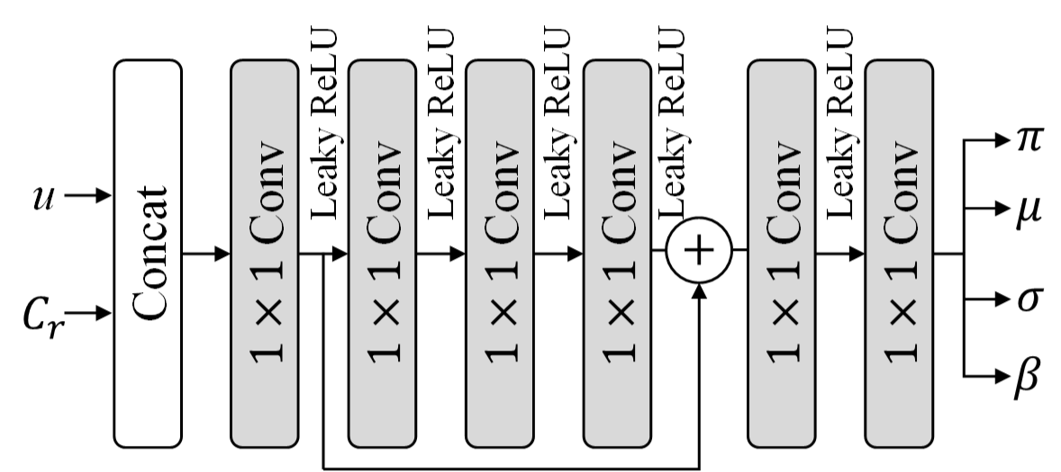
We model the PMF of $r_{i,c}$ with discrete logistic mixture likelihood [20] and propose a sub-network to estimate the corresponding entropy parameters, including mixture weights $\pi_{i}^{k}$, means $\mu_{i,c}^{k}$, variances $\sigma_{i,c}^{k}$ and mixture coefficients $\beta_{i,t}$. $k$ denotes the index of the $k$-th logistic distribution. $t$ denotes the channel index of $\beta$. The network architecture of the entropy model is shown in Fig. 4. We utilize a mixture of $K=5$ logistic distributions. The channel autoregressive scheme over $r_{i,1},r_{i,2},r_{i,3}$ is implemented by updating the means using:

With $\pi_{i}^{k}$, $\tilde{\mu}_{i,c}^{k}$ and $\sigma_{i,c}^{k}$, we have

where $\operatorname*{logistic}(\cdot)$ denotes the logistic distribution. For discrete $r_{i,c}$, we evaluate $p_{\boldsymbol{\theta}}(r_{i,c}|r_{i,<c},u_{i},C_{r_{i}})$ as [20]:

where $S(\cdot)$ denotes the sigmoid function. $r_{i,c}^{+}=r_{i,c}+0.5$ and $r_{i,c}^{-}=r_{i,c}-0.5$. The probability inference scheme of $\mathbf{r}$ is sketched in Fig. 5a.

We finally introduce SQRC to realize scalable near-lossless image compression with variable $\ell_{\infty}$ bound $\tau\in\{1,2,\ldots\}$. Though near-lossless image compression given a specific $\tau$ can be realized by optimizing (10), this $\tau$-specific scheme in Fig. 5b leads to two problems:

• •

  Relaxation problem of residual quantization. Unlike rounding quantization, the bin size of the residual quantization (9) is much larger. Moreover, the original residuals are not uniformly distributed in each bin, and thus cannot be relaxed by adding uniform noise.

• •

  Storage problem of multiple networks. To deploy the near-lossless codec, we have to transmit and store multiple networks for different $\tau$’s, which is storage-inefficient.

Instead, we propose a scalable near-lossless image compression scheme, which can circumvent the relaxation of residual quantization and utilize a single network to satisfy variable $\ell_{\infty}$ error bound $\tau\in\{1,2,\ldots\}$. Specifically, the scalable compression scheme is based on the learned lossless compression with the DLPR coding framework. We keep the lossy reconstruction ${\tilde{\mathbf{x}}}$ fixed and quantize the original residual $\mathbf{r}$ to ${\hat{\mathbf{r}}}$ with variable $\tau$’s by (9). To encode the quantized ${\hat{\mathbf{r}}}$, we can derive the PMF of ${\hat{\mathbf{r}}}$ from the learned PMF of the original $\mathbf{r}$. Given $\tau$ and the learned PMF $p_{\boldsymbol{\theta}}(r_{i,c}|r_{i,<c},u_{i},C_{r_{i}})$ of original $r_{i,c}$, the PMF $\hat{p}_{\boldsymbol{\theta}}(\hat{r}_{i,c}|r_{i,<c},u_{i},C_{r_{i}})$ of quantized $\hat{r}_{i,c}$ can be computed by the following PMF quantization:

We show an illustrative example in Fig. 6. Together with (14) and (15), we can derive the probability model $\hat{p}_{\boldsymbol{\theta}}({\hat{\mathbf{r}}}|\mathbf{u},C_{\mathbf{r}})$ of ${\hat{\mathbf{r}}}$, which is optimal given the learned $p_{\boldsymbol{\theta}}(\mathbf{r}|\mathbf{u},C_{\mathbf{r}})$ of $\mathbf{r}$. The resulting cost of encoding ${\hat{\mathbf{r}}}$, denoted by $R^{\tau}_{{\hat{\mathbf{r}}}}$, is reduced significantly with the increase of $\tau$.

However, encoding ${\hat{\mathbf{r}}}$ with $\hat{p}_{\boldsymbol{\theta}}({\hat{\mathbf{r}}}|\mathbf{u},C_{\mathbf{r}})$ results in undecodable bitstreams, since the original residual $\mathbf{r}$ is unknown to the decoder. $\hat{p}_{\boldsymbol{\theta}}(\hat{r}_{i,c}|r_{i,<c},u_{i},C_{r_{i}})$ cannot be evaluated without $r_{i,<c}$ and causal context $C_{r_{i}}$. Instead, we can evaluate PMF using the quantized residual ${\hat{\mathbf{r}}}$, i.e., we evaluate $p_{\boldsymbol{\theta}}(r_{i,c}|\hat{r}_{i,<c},u_{i},C_{\hat{r}_{i}})$ and derive $\hat{p}_{\boldsymbol{\theta}}(\hat{r}_{i,c}|\hat{r}_{i,<c},u_{i},C_{\hat{r}_{i}})$ with (19), leading to $\hat{p}_{\boldsymbol{\theta}}({\hat{\mathbf{r}}}|\mathbf{u},C_{\hat{\mathbf{r}}})$ for the encoding of ${\hat{\mathbf{r}}}$. Because of the mismatch between training (with $\mathbf{r}$) and inference (with ${\hat{\mathbf{r}}}$) phases, it leads to biased PMF $p_{\boldsymbol{\theta}}(r_{i,c}|\hat{r}_{i,<c},u_{i},C_{\hat{r}_{i}})$, $\hat{p}_{\boldsymbol{\theta}}(\hat{r}_{i,c}|\hat{r}_{i,<c},u_{i},C_{\hat{r}_{i}})$ and $\hat{p}_{\boldsymbol{\theta}}({\hat{\mathbf{r}}}|\mathbf{u},C_{\hat{\mathbf{r}}})$. The above probability inference scheme is sketched in Fig. 5c.

SQRC for Bias Correction: Because of the discrepancy between the oracle $\hat{p}_{\boldsymbol{\theta}}({\hat{\mathbf{r}}}|\mathbf{u},C_{\mathbf{r}})$ and the biased $\hat{p}_{\boldsymbol{\theta}}({\hat{\mathbf{r}}}|\mathbf{u},C_{\hat{\mathbf{r}}})$, encoding ${\hat{\mathbf{r}}}$ with $\hat{p}_{\boldsymbol{\theta}}({\hat{\mathbf{r}}}|\mathbf{u},C_{\hat{\mathbf{r}}})$ degrades the compression performance. In order to tackle this problem, we propose SQRC for bias correction to close the gap between the oracle $\hat{p}_{\boldsymbol{\theta}}({\hat{\mathbf{r}}}|\mathbf{u},C_{\mathbf{r}})$ and the biased $\hat{p}_{\boldsymbol{\theta}}({\hat{\mathbf{r}}}|\mathbf{u},C_{\hat{\mathbf{r}}})$, while the resulting bitstreams are still decodable. The components of SQRC are illustrated in Fig. 1. The masked convolutional layer in SQRC is shared with that in RC. The conditional entropy model has the same network architecture as the entropy model illustrated in Fig. 4, but replaces the convolutional layers with the conditional convolutional layers [19, 60] illustrated in Fig. 7.

The probability inference scheme with SQRC is sketched in Fig. 5d. For $\tau=0$, we still select the entropy model in RC to estimate $p_{\boldsymbol{\theta}}(\mathbf{r}|\mathbf{u},C_{\mathbf{r}})$ to encode $\mathbf{r}$. For $\tau\in\{1,2,\ldots,N\}$, we select the conditional entropy model in SQRC to estimate $p_{\boldsymbol{\varphi}}(\mathbf{r}|\mathbf{u},C_{{\hat{\mathbf{r}}}},\tau)$ conditioned on $\tau$. We then derive $\hat{p}_{\boldsymbol{\varphi}}({\hat{\mathbf{r}}}|\mathbf{u},C_{{\hat{\mathbf{r}}}},\tau)$ with (19) to encode ${\hat{\mathbf{r}}}$, where ${\boldsymbol{\varphi}}$ denote the parameters of SQRC. As $\hat{p}_{\boldsymbol{\varphi}}({\hat{\mathbf{r}}}|\mathbf{u},C_{{\hat{\mathbf{r}}}},\tau)$ approximates the oracle $\hat{p}_{\boldsymbol{\theta}}({\hat{\mathbf{r}}}|\mathbf{u},C_{\mathbf{r}})$ better than the biased $\hat{p}_{\boldsymbol{\theta}}({\hat{\mathbf{r}}}|\mathbf{u},C_{\hat{\mathbf{r}}})$, the compression performance can be improved. Since evaluating $\hat{p}_{\boldsymbol{\varphi}}({\hat{\mathbf{r}}}|\mathbf{u},C_{{\hat{\mathbf{r}}}},\tau)$ is independent of $\mathbf{r}$, the resulting bitstreams are decodable. In experiments, we demonstrate that the proposed scalable near-lossless compression scheme with SQRC in Fig. 5d can outperform both the $\tau$-specific near-lossless scheme in Fig. 5b and the scalable near-lossless compression scheme without SQRC in Fig. 5c.

The full loss function for jointly optimizing LIC and RC, i.e., DLPR coding for lossless image compression, is

where ${\boldsymbol{\theta}}$ and ${\boldsymbol{\phi}}$ are the learned parameters of LIC and RC. Besides rate terms $R_{{\hat{\mathbf{y}}},{\hat{\mathbf{z}}}}$ in (11) and $R_{\mathbf{r}}$ in (13), we further introduce a distortion term $D_{ls}(\mathbf{x},{\tilde{\mathbf{x}}})$ to minimize the mean square error (MSE) between the raw image $\mathbf{x}$ and its lossy reconstruction ${\tilde{\mathbf{x}}}$:

As discussed in [25], minimizing MSE loss is equivalent to learn a LIC that fits residual $\mathbf{r}$ to a factorized Gaussian distribution. However, the discrepancy between the real distribution of $\mathbf{r}$ and the factorized Gaussian distribution is usually large. Therefore, we utilize a sophisticated discrete logistic mixture likelihood model to encode $\mathbf{r}$ in our DLPR coding framework.

The $\lambda$ in (20) is a “rate-distortion” trade-off parameter between the lossless compression rate and the MSE distortion. When $\lambda=0$, the loss function (20) is consistent with the theoretical DLPR coding formulation (7), and ${\tilde{\mathbf{x}}}$ becomes a latent variable without any constraints. In experiments, we study the effects of $\lambda$’s on the lossless and near-lossless image compression performance. We set $\lambda=0$ leading to the best lossless image compression, while set $\lambda=0.03$ leading to robust near-lossless image compression with variable $\tau$’s.

For training SQRC, we generate random $\tau\in\{1,2,\ldots,N\}$ and quantize $\mathbf{r}$ to ${\hat{\mathbf{r}}}$ with (9). Given $\mathbf{u}$ and the extracted context $C_{\hat{\mathbf{r}}}$ from quantized ${\hat{\mathbf{r}}}$, we use the conditional entropy model to estimate $-\log p_{\boldsymbol{\varphi}}(\mathbf{r}|\mathbf{u},C_{{\hat{\mathbf{r}}}},\tau)$ conditioned on different $\tau$’s, and minimize

where ${\boldsymbol{\varphi}}$ denote the learned parameters of the conditional entropy model. $-\log p_{\boldsymbol{\theta}}(\mathbf{r}|\mathbf{u},C_{\mathbf{r}})$ is estimated by the entropy model in RC. $\mathcal{L}({\boldsymbol{\varphi}})$ can be considered as an approximate KL-divergence or relative entropy [55] between $p_{\boldsymbol{\theta}}(\mathbf{r}|\mathbf{u},C_{\mathbf{r}})$ and $p_{\boldsymbol{\varphi}}(\mathbf{r}|\mathbf{u},C_{{\hat{\mathbf{r}}}},\tau)$.

SQRC is trained together with LIC and RC, but minimizing (22) only updates the parameters of the conditional entropy model as shown in Fig. 1. The masked convolutional layer is shared with that in RC, and thus can be updated by minimizing (20). This leads to three advantages: 1) We can achieve the target conditional entropy model to close the gap between training with $\mathbf{r}$ and inference with ${\hat{\mathbf{r}}}$; 2) We can circumvent the aforementioned relaxation problem of residual quantization; 3) We can avoid degrading the estimation of $p_{\boldsymbol{\theta}}(\mathbf{r}|\mathbf{u},C_{\mathbf{r}})$ in RC caused by training with randomly generated $\tau$. Because the entropy model in RC receives the context $C_{\mathbf{r}}$ extracted from the original residual $\mathbf{r}$, $p_{\boldsymbol{\theta}}(\mathbf{r}|\mathbf{u},C_{\mathbf{r}})$ approximates the true distribution $p(\mathbf{r}|{\tilde{\mathbf{x}}},{\hat{\mathbf{y}}})$ better than $p_{\boldsymbol{\varphi}}(\mathbf{r}|\mathbf{u},C_{{\hat{\mathbf{r}}}},\tau)$. Thus, $-\log p_{\boldsymbol{\theta}}(\mathbf{r}|\mathbf{u},C_{\mathbf{r}})$ is the lower bound of $-\log p_{\boldsymbol{\varphi}}(\mathbf{r}|\mathbf{u},C_{{\hat{\mathbf{r}}}},\tau)$ on average.

Generally, autoregressive models suffer from serialized decoding and cannot be efficiently implemented on GPUs. Given an $H\times W$ image, we need to compute $HW$ times context model to decode all pixels sequentially. In lossy image compression, checkerboard context model [45] and channel-wise context model [44] were introduced to accelerate the probability inference of latent variables. However, these two context models are too weak for our residual coding and result in significant performance degradation, without the help of transform coding.

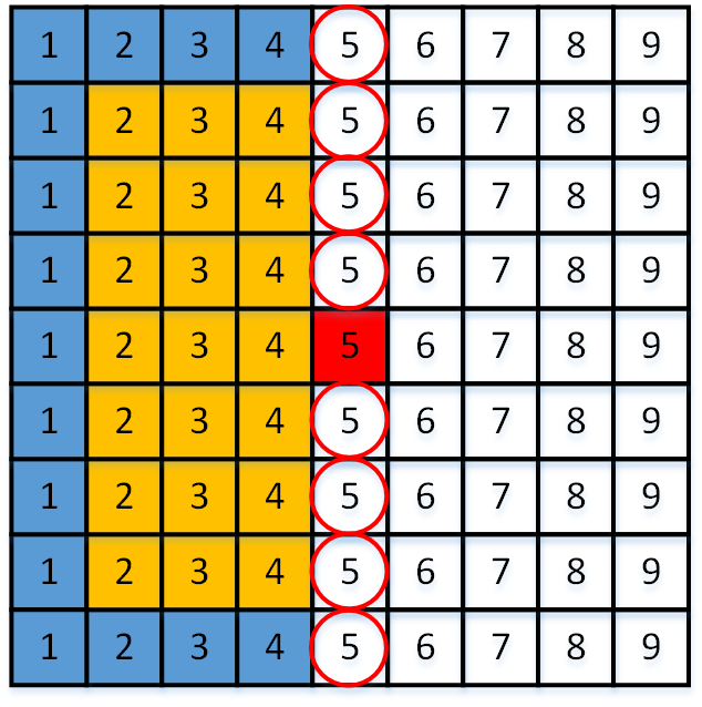
To improve the parallelization of residual coding, we first adopt a common operation to split an $H\times W$ image into multiple non-overlapping $P\times P$ patches and code all $P\times P$ patches in parallel, reducing $HW$ times sequential context computations to $P^{2}$ times. We next propose a novel design of context coding to improve the algorithm parallelization given the $P\times P$ patches and $k\times k$ mask convolution, as illustrated in Fig. 8. Assuming that $P=9$ and $k=7$, we need $P^{2}=81$ sequential decoding steps in raster scan order for the commonly used context model shown in Fig. 8a. The number in each pixel denotes the time step $t$ at which the pixel is decoded. Since $P>\lceil\frac{k}{2}\rceil$ is usually satisfied, the currently decoded pixel only depends on some of the previously decoded pixels. For example, the red pixel is decoded currently and the yellow pixels are its context. The blue pixels are previously decoded pixels but are not included in the context of the red pixel. Hence, there are pixels that can be potentially decoded in parallel by revising the scan order. By using $\frac{180}{\pi}\cdot\arctan(\frac{2}{k+1})$ degree parallel scan, the pixels with the same number $t$ can be decoded simultaneously, as shown in Fig. 8b. The number of decoding steps is reduced from $P^{2}$ to $\frac{k+3}{2}\cdot P-\frac{k+1}{2}$. In this case, we use $14.04^{\circ}$ parallel scan, leading to $5P-4=41$ sequential decoding steps. The similar scan order was also used in [61]. Moreover, we can remove one context pixel in the upper right of the currently decoded pixel. The newly designed context model leads to $\frac{180}{\pi}\cdot\arctan(\frac{2}{k-1})$ degree parallel scan and reduces decoding steps to $\frac{k+1}{2}\cdot P-\frac{k-1}{2}$. As shown in Fig. 8c, we use $18.43^{\circ}$ parallel scan and $4P-3=33$ decoding steps with this context model. When more upper-right context pixels are removed, the coding parallelization can be further improved while the compression performance is gradually compromised on. As shown in Fig. 8d, the context model leads to $\frac{180}{\pi}\cdot\arctan(\frac{2}{k-3})$ degree parallel scan and $\frac{k-1}{2}\cdot P-\frac{k-3}{2}$ decoding steps, i.e., $26.57^{\circ}$ parallel scan and $3P-2=25$ decoding steps in our example. When $45^{\circ}$ parallel scan is reached, this special case is the zig-zag scan [43] and we need $2P-1=17$ decoding steps, as shown in Fig. 8e. Finally, the fastest case is shown in Fig. 8f. We can use $90^{\circ}$ parallel scan and only $P=9$ decoding steps.

In summary, the proposed design of context coding demonstrates that: given $P\times P$ image patches and $k\times k$ mask convolution with $P>\lceil\frac{k}{2}\rceil$, we can design a series of context models $\{M^{(k+3)/2}_{k},M^{(k+1)/2}_{k},\ldots,M^{1}_{k}\}$ leading to $\{\frac{k+3}{2}\cdot P-\frac{k+1}{2},\frac{k+1}{2}\cdot P-\frac{k-1}{2},\ldots,P\}$ parallel decoding steps, by gradually adjusting the context pixels. The corresponding scan angles are $\{\frac{180}{\pi}\cdot\arctan(\frac{2}{k+1}),\frac{180}{\pi}\cdot\arctan(\frac{2}{k-1}),\ldots,90^{\circ}\}$, respectively. In experiments, we set $P=64$, $k=7$ and select the context model $M^{3}_{7}$ shown in Fig. 8d. The $M^{3}_{7}$ enjoys almost the same compression performance as $M_{7}^{5}$ in Fig. 8a and Fig. 8b, but needs much fewer coding steps.

Since the pixels of both a raw image $\mathbf{x}$ and its lossy reconstruction ${\tilde{\mathbf{x}}}$ are in the interval $[0,255]$, the element $r_{i,c}$ of the corresponding residual $\mathbf{r}$ is in the interval $[-255,255]$. To entropy coding each $r_{i,c}$, we need to compute and utilize PMF with $511$ elements, which is relatively large and slows down the entropy coding process.

In practice, the theoretical interval $[-255,255]$ of $r_{i,c}$ can hardly be filled up. Hence, we can compute and record $r_{\min}=\min_{i,c}r_{i,c}$ and $r_{\max}=\max_{i,c}r_{i,c}$ of each image, and reduce the domain of PMF to the adaptive interval $[r_{\min},r_{\max}]$ with $r_{\max}-r_{\min}+1$ elements. The overheads of recording the $r_{\min}$ and $r_{\max}$ can be amortized and ignored. For near-lossless image compression with $\tau>0$, we can similarly compute and record the quantized $\hat{r}_{\min}=\min_{i,c}\hat{r}_{i,c}$ and $\hat{r}_{\max}=\max_{i,c}\hat{r}_{i,c}$ of each image, and the domain of the quantized PMF can be further reduced to the adaptive interval $\{\hat{r}_{\min},\hat{r}_{\min}+2\tau+1,\hat{r}_{\min}+2\cdot(2\tau+1),\ldots,\hat{r}_{\max}\}$, i.e., $\frac{\hat{r}_{\max}-\hat{r}_{\min}}{2\tau+1}+1$ elements in total. The reduction of residual intervals can significantly accelerate the entropy coding on average.

References

- [1] C. E. Shannon, “A mathematical theory of communication,” The Bell system technical journal, vol. 27, no. 3, pp. 379–423, 1948.
- [2] M. J. Weinberger, G. Seroussi, and G. Sapiro, “The loco-i lossless image compression algorithm: Principles and standardization into jpeg-ls,” IEEE Transactions on Image Processing, vol. 9, no. 8, pp. 1309–1324, 2000.
- [3] X. Wu and N. Memon, “Context-based, adaptive, lossless image coding,” IEEE Transactions on Communications, vol. 45, no. 4, pp. 437–444, 1997.
- [4] J. Sneyers and P. Wuille, “Flif: Free lossless image format based on maniac compression,” in IEEE International Conference on Image Processing. IEEE, 2016, pp. 66–70.
- [5] J. Alakuijala, R. Van Asseldonk, S. Boukortt, M. Bruse, I.-M. Comsa, M. Firsching, T. Fischbacher, E. Kliuchnikov, S. Gomez, R. Obryk et al., “Jpeg xl next-generation image compression architecture and coding tools,” in Applications of Digital Image Processing XLII, vol. 11137. SPIE, 2019, pp. 112–124.
- [6] R. Ansari, N. D. Memon, and E. Ceran, “Near-lossless image compression techniques,” Journal of Electronic Imaging, vol. 7, no. 3, pp. 486 – 494, 1998.
- [7] L. Ke and M. W. Marcellin, “Near-lossless image compression: minimum-entropy, constrained-error dpcm,” IEEE Transactions on Image Processing, vol. 7, no. 2, pp. 225–228, 1998.
- [8] W. Xiaolin and P. Bao, “ constrained high-fidelity image compression via adaptive context modeling,” IEEE Transactions on Image Processing, vol. 9, no. 4, pp. 536–542, 2000.
- [9] Y. Hu, W. Yang, Z. Ma, and J. Liu, “Learning end-to-end lossy image compression: A benchmark,” IEEE Transactions on Pattern Analysis and Machine Intelligence, vol. 44, no. 8, pp. 4194–4211, 2022.
- [10] F. Mentzer, E. Agustsson, M. Tschannen, R. Timofte, and L. V. Gool, “Practical full resolution learned lossless image compression,” in IEEE Conference on Computer Vision and Pattern Recogition, 2019, pp. 10 621–10 630.
- [11] F. Mentzer, L. Van Gool, and M. Tschannen, “Learning better lossless compression using lossy compression,” in IEEE Conference on Computer Vision and Pattern Recogition, 2020.
- [12] F. H. Kingma, P. Abbeel, and J. Ho, “Bit-swap: Recursive bits-back coding for lossless compression with hierarchical latent variables,” in International Conference on Machine Learning, 2019.
- [13] J. Townsend, T. Bird, J. Kunze, and D. Barber, “Hilloc: Lossless image compression with hierarchical latent variable models,” in International Conference on Learning Representations, 2020.
- [14] E. Hoogeboom, J. Peters, R. van den Berg, and M. Welling, “Integer discrete flows and lossless compression,” in Advances in Neural Information Processing Systems, 2019, pp. 12 134–12 144.
- [15] J. Ho, E. Lohn, and P. Abbeel, “Compression with flows via local bits-back coding,” in Advances in Neural Information Processing Systems, vol. 32, 2019.
- [16] S. Zhang, C. Zhang, N. Kang, and Z. Li, “ivpf: Numerical invertible volume preserving flow for efficient lossless compression,” in IEEE Conference on Computer Vision and Pattern Recogition, 2021, pp. 620–629.
- [17] S. Zhang, N. Kang, T. Ryder, and Z. Li, “iflow: Numerically invertible flows for efficient lossless compression via a uniform coder,” in Advances in Neural Information Processing Systems, vol. 34, 2021.
- [18] A. v. d. Oord, N. Kalchbrenner, and K. Kavukcuoglu, “Pixel recurrent neural networks,” in International Conference on Machine Learning. JMLR.org, 2016, pp. 1747–1756.
- [19] A. van den Oord, N. Kalchbrenner, L. Espeholt, O. Vinyals, and A. Graves, “Conditional image generation with pixelcnn decoders,” in Advances in Neural Information Processing Systems, 2016, pp. 4790–4798.
- [20] T. Salimans, A. Karpathy, X. Chen, and D. P. Kingma, “Pixelcnn++: Improving the pixelcnn with discretized logistic mixture likelihood and other modifications,” in International Conference on Learning Representations, 2017.
- [21] I. Kobyzev, S. J. Prince, and M. A. Brubaker, “Normalizing flows: An introduction and review of current methods,” IEEE Transactions on Pattern Analysis and Machine Intelligence, vol. 43, no. 11, pp. 3964–3979, 2020.
- [22] D. P. Kingma and M. Welling, “Auto-encoding variational bayes,” in International Conference on Learning Representations, 2014.
- [23] Y. Bai, X. Liu, W. Zuo, Y. Wang, and X. Ji, “Learning scalable -constrained near-lossless image compression via joint lossy image and residual compression,” in Proceedings of the IEEE/CVF Conference on Computer Vision and Pattern Recognition, June 2021, pp. 11 946–11 955.
- [24] J. Ballé, V. Laparra, and E. P. Simoncelli, “End-to-end optimized image compression,” in International Conference on Learning Representations, 2017.
- [25] J. Ballé, D. Minnen, S. Singh, S. J. Hwang, and N. Johnston, “Variational image compression with a scale hyperprior,” in International Conference on Learning Representations, 2018.
- [26] J. Townsend, T. Bird, and D. Barber, “Practical lossless compression with latent variables using bits back coding,” in International Conference on Learning Representations, 2019.
- [27] G. Toderici, S. M. O’Malley, S. J. Hwang, D. Vincent, D. Minnen, S. Baluja, M. Covell, and R. Sukthankar, “Variable rate image compression with recurrent neural networks,” in International Conference on Learning Representations, 2016.
- [28] G. Toderici, D. Vincent, N. Johnston, S. Jin Hwang, D. Minnen, J. Shor, and M. Covell, “Full resolution image compression with recurrent neural networks,” in IEEE Conference on Computer Vision and Pattern Recogition, 2017, pp. 5306–5314.
- [29] N. Johnston, D. Vincent, D. Minnen, M. Covell, S. Singh, T. Chinen, S. J. Hwang, J. Shor, and G. Toderici, “Improved lossy image compression with priming and spatially adaptive bit rates for recurrent networks,” in IEEE Conference on Computer Vision and Pattern Recogition, 2018, pp. 4385–4393.
- [30] L. Theis, W. Shi, A. Cunningham, and F. Huszár, “Lossy image compression with compressive autoencoders,” in International Conference on Learning Representations, 2017.
- [31] V. K. Goyal, “Theoretical foundations of transform coding,” IEEE Signal Processing Magazine, vol. 18, no. 5, pp. 9–21, 2001.
- [32] Z. Wang, E. P. Simoncelli, and A. C. Bovik, “Multiscale structural similarity for image quality assessment,” in The Thrity-Seventh Asilomar Conference on Signals, Systems & Computers, 2003, vol. 2. Ieee, 2003, pp. 1398–1402.
- [33] Z. Cheng, H. Sun, M. Takeuchi, and J. Katto, “Learned image compression with discretized gaussian mixture likelihoods and attention modules,” in IEEE Conference on Computer Vision and Pattern Recogition, 2020, pp. 7939–7948.
- [34] H. Ma, D. Liu, N. Yan, H. Li, and F. Wu, “End-to-end optimized versatile image compression with wavelet-like transform,” IEEE Transactions on Pattern Analysis and Machine Intelligence, vol. 44, no. 3, pp. 1247–1263, 2022.
- [35] Y. Zhu, Y. Yang, and T. Cohen, “Transformer-based transform coding,” in International Conference on Learning Representations, 2022.
- [36] M. Li, W. Zuo, S. Gu, J. You, and D. Zhang, “Learning content-weighted deep image compression,” IEEE Transactions on Pattern Analysis and Machine Intelligence, 2020.
- [37] F. Mentzer, E. Agustsson, M. Tschannen, R. Timofte, and L. V. Gool, “Conditional probability models for deep image compression,” in IEEE Conference on Computer Vision and Pattern Recogition, 2018, pp. 4394–4402.
- [38] E. Agustsson, F. Mentzer, M. Tschannen, L. Cavigelli, R. Timofte, L. Benini, and L. V. Gool, “Soft-to-hard vector quantization for end-to-end learning compressible representations,” in Advances in Neural Information Processing Systems, vol. 30, 2017.
- [39] Y. Hu, W. Yang, and J. Liu, “Coarse-to-fine hyper-prior modeling for learned image compression,” in Proceedings of the AAAI Conference on Artificial Intelligence, vol. 34, no. 07, 2020, pp. 11 013–11 020.
- [40] D. Minnen, J. Ballé, and G. D. Toderici, “Joint autoregressive and hierarchical priors for learned image compression,” in Advances in Neural Information Processing Systems, 2018, pp. 10 771–10 780.
- [41] Y. Qian, Z. Tan, X. Sun, M. Lin, D. Li, Z. Sun, H. Li, and R. Jin, “Learning accurate entropy model with global reference for image compression,” in International Conference on Learning Representations, 2021.
- [42] Y. Qian, M. Lin, X. Sun, Z. Tan, and R. Jin, “Entroformer: A transformer-based entropy model for learned image compression,” in International Conference on Learning Representations, 2022.
- [43] M. Li, K. Ma, J. You, D. Zhang, and W. Zuo, “Efficient and effective context-based convolutional entropy modeling for image compression,” IEEE Transactions on Image Processing, vol. 29, pp. 5900–5911, 2020.
- [44] D. Minnen and S. Singh, “Channel-wise autoregressive entropy models for learned image compression,” in IEEE International Conference on Image Processing. IEEE, 2020, pp. 3339–3343.
- [45] D. He, Y. Zheng, B. Sun, Y. Wang, and H. Qin, “Checkerboard context model for efficient learned image compression,” in IEEE Conference on Computer Vision and Pattern Recogition, 2021.
- [46] I. H. Witten, R. M. Neal, and J. G. Cleary, “Arithmetic coding for data compression,” Communications of the ACM, vol. 30, no. 6, pp. 520–540, 1987.
- [47] J. Duda, “Asymmetric numeral systems,” arXiv preprint arXiv:0902.0271, 2009.
- [48] S. Reed, A. Oord, N. Kalchbrenner, S. G. Colmenarejo, Z. Wang, Y. Chen, D. Belov, and N. Freitas, “Parallel multiscale autoregressive density estimation,” in International Conference on Machine Learning. PMLR, 2017, pp. 2912–2921.
- [49] M. Zhang, A. Zhang, and S. McDonagh, “On the out-of-distribution generalization of probabilistic image modelling,” in Advances in Neural Information Processing Systems, vol. 34, 2021.
- [50] R. v. d. Berg, A. A. Gritsenko, M. Dehghani, C. K. Sønderby, and T. Salimans, “Idf++: Analyzing and improving integer discrete flows for lossless compression,” in International Conference on Learning Representations, 2021.
- [51] F. Bellard, “BPG image format,” https://bellard.org/bpg/.
-
[52]
Google, “Webp image format,”
https://developers.google.com/
speed/webp/. - [53] K. Chen and T. V. Ramabadran, “Near-lossless compression of medical images through entropy-coded dpcm,” IEEE Transactions on Medical Imaging, vol. 13, no. 3, pp. 538–548, 1994.
- [54] X. Zhang and X. Wu, “Ultra high fidelity deep image decompression with -constrained compression,” IEEE Transactions on Image Processing, vol. 30, pp. 963–975, 2021.
- [55] T. M. Cover and J. A. Thomas, Elements of Information Theory (Wiley Series in Telecommunications and Signal Processing). USA: Wiley-Interscience, 2006.
- [56] K. He, X. Zhang, S. Ren, and J. Sun, “Deep residual learning for image recognition,” in IEEE Conference on Computer Vision and Pattern Recogition, 2016, pp. 770–778.
- [57] Y. Zhang, K. Li, K. Li, B. Zhong, and Y. Fu, “Residual non-local attention networks for image restoration,” in International Conference on Learning Representations, 2019.
- [58] Z. Liu, Y. Lin, Y. Cao, H. Hu, Y. Wei, Z. Zhang, S. Lin, and B. Guo, “Swin transformer: Hierarchical vision transformer using shifted windows,” in International Conference on Computer Vision, 2021, pp. 10 012–10 022.
- [59] J. Ballé, V. Laparra, and E. P. Simoncelli, “Density modeling of images using a generalized normalization transformation,” in International Conference on Learning Representations, 2016.
- [60] Y. Choi, M. El-Khamy, and J. Lee, “Variable rate deep image compression with a conditional autoencoder,” in International Conference on Computer Vision, 2019, pp. 3146–3154.
- [61] M. Zhang, J. Townsend, N. Kang, and D. Barber, “Parallel neural local lossless compression,” arXiv preprint arXiv:2201.05213, 2022.
- [62] E. Agustsson and R. Timofte, “NTIRE 2017 challenge on single image super-resolution: dataset and study,” in IEEE Conference on Computer Vision and Pattern Recogition Workshop, July 2017.
- [63] D. P. Kingma and J. Ba, “Adam: A method for stochastic optimization,” in International Conference on Learning Representations, 2015.
- [64] P. Chrabaszcz, I. Loshchilov, and F. Hutter, “A downsampled variant of imagenet as an alternative to the cifar datasets,” arXiv preprint arXiv:1707.08819, 2017.
- [65] J. Deng, W. Dong, R. Socher, L.-J. Li, K. Li, and L. Fei-Fei, “Imagenet: A large-scale hierarchical image database,” in IEEE Conference on Computer Vision and Pattern Recogition. Ieee, 2009, pp. 248–255.
- [66] E. Kodak, “Kodak lossless true color image suite (photocd pcd0992),” http://r0k.us/graphics/kodak/, 1993.
- [67] J. Borovec, J. Kybic, I. Arganda-Carreras, D. V. Sorokin, G. Bueno, A. V. Khvostikov, S. Bakas, I. Eric, C. Chang, S. Heldmann et al., “Anhir: automatic non-rigid histological image registration challenge,” IEEE Transactions on Medical Imaging, vol. 39, no. 10, pp. 3042–3052, 2020.
- [68] A. Skodras, C. Christopoulos, and T. Ebrahimi, “The jpeg 2000 still image compression standard,” IEEE Signal Processing Magazine, vol. 18, no. 5, pp. 36–58, 2001.
- [69] G. K. Wallace, “The jpeg still picture compression standard,” IEEE Transactions on Consumer Electronics, vol. 38, no. 1, pp. xviii–xxxiv, 1992.
- [70] J.-R. Ohm and G. J. Sullivan, “Versatile video coding–towards the next generation of video compression,” in Picture Coding Symposium, 2018.
- [71] I. Gulrajani, K. Kumar, F. Ahmed, A. A. Taiga, F. Visin, D. Vazquez, and A. Courville, “Pixelvae: A latent variable model for natural images,” in International Conference on Learning Representations, 2017.
![[Uncaptioned image]](https://cdn.awesomepapers.org/papers/ed9bf348-377a-4d95-ac90-836ad94a0144/Yuanchao_Bai.jpg) |
Yuanchao Bai (Member, IEEE) received the B.S. degree in software engineering from Dalian University of Technology, Liaoning, China, in 2013. He received the Ph.D. degree in computer science from Peking University, Beijing, China, in 2020. He was a postdoctoral fellow in Peng Cheng Laboratory, Shenzhen, China, from 2020 to 2022. He is currently an assistant professor with the School of Computer Science and Technology, Harbin Institute of Technology, Harbin, China. His research interests include image/video compression and processing, deep unsupervised learning, and graph signal processing. |
![[Uncaptioned image]](https://cdn.awesomepapers.org/papers/ed9bf348-377a-4d95-ac90-836ad94a0144/Xianming.jpg) |
Xianming Liu (Member, IEEE) is a Professor with the School of Computer Science and Technology, Harbin Institute of Technology (HIT), Harbin, China. He received the B.S., M.S., and Ph.D degrees in computer science from HIT, in 2006, 2008 and 2012, respectively. In 2011, he spent half a year at the Department of Electrical and Computer Engineering, McMaster University, Canada, as a visiting student, where he then worked as a post-doctoral fellow from December 2012 to December 2013. He worked as a project researcher at National Institute of Informatics (NII), Tokyo, Japan, from 2014 to 2017. He has published over 60 international conference and journal publications, including top IEEE journals, such as T-IP, T-CSVT, T-IFS, T-MM, T-GRS; and top conferences, such as CVPR, IJCAI and DCC. He is the receipt of IEEE ICME 2016 Best Student Paper Award. |
![[Uncaptioned image]](https://cdn.awesomepapers.org/papers/ed9bf348-377a-4d95-ac90-836ad94a0144/KaiWang.jpg) |
Kai Wang received the B.S. degree in software engineering from Harbin Engineering University, Harbin, China, in 2020 and received the M.S. degree of electronic information in software engineering from Harbin Institute of Technology, Harbin, China, in 2022. He is currently pursuing the docter degree in electronic information in Harbin Institute of Technology, Harbin, China. His research interests include image/video compression and deep learning. |
![[Uncaptioned image]](https://cdn.awesomepapers.org/papers/ed9bf348-377a-4d95-ac90-836ad94a0144/Xiangyang_Ji.jpg) |
Xiangyang Ji (Member, IEEE) received the B.S. degree in materials science and the M.S. degree in computer science from the Harbin Institute of Technology, Harbin, China, in 1999 and 2001, respectively, and the Ph.D. degree in computer science from the Institute of Computing Technology, Chinese Academy of Sciences, Beijing, China. He joined Tsinghua University, Beijing, in 2008, where he is currently a Professor with the Department of Automation, School of Information Science and Technology. He has authored over 100 referred conference and journal papers. His current research interests include signal processing, image/video compressing, and intelligent imaging. |
![[Uncaptioned image]](https://cdn.awesomepapers.org/papers/ed9bf348-377a-4d95-ac90-836ad94a0144/wu_xiaolin.jpg) |
Xiaolin Wu (Fellow, IEEE) received the B.Sc. degree in computer science from Wuhan University, China, in 1982, and the Ph.D. degree in computer science from the University of Calgary, Canada, in 1988. He started his academic career in 1988. He was a Faculty Member with Western University, Canada, and New York Polytechnic University (NYU-Poly), USA. He is currently with McMaster University, Canada, where he is a Distinguished Engineering Professor and holds an NSERC Senior Industrial Research Chair. His research interests include image processing, data compression, digital multimedia, low-level vision, and network-aware visual communication. He has authored or coauthored more than 300 research articles and holds four patents in these fields. He served on technical committees of many IEEE international conferences/workshops on image processing, multimedia, data compression, and information theory. He was a past Associated Editor of IEEE TRANSACTIONS ON MULTIMEDIA. He is also an Associated Editor of IEEE TRANSACTIONS ON IMAGE PROCESSING. |
![[Uncaptioned image]](https://cdn.awesomepapers.org/papers/ed9bf348-377a-4d95-ac90-836ad94a0144/WenGao.jpg) |
Wen Gao (Fellow, IEEE) received the Ph.D. degree in electronics engineering from The University of Tokyo, Japan, in 1991. He is currently a Boya Chair Professor in computer science at Peking University. He is the Director of Peng Cheng Laboratory, Shenzhen. Before joining Peking University, he was a Professor with Harbin Institute of Technology from 1991 to 1995. From 1996 to 2006, he was a Professor at the Institute of Computing Technology, Chinese Academy of Sciences. He has authored or coauthored five books and over 1000 technical articles in refereed journals and conference proceedings in the areas of image processing, video coding and communication, computer vision, multimedia retrieval, multimodal interface, and bioinformatics. He served on the editorial boards for several journals, such as ACM CSUR, IEEE TRANSACTIONS ON IMAGE PROCESSING (TIP), IEEE TRANSACTIONS ON CIRCUITS AND SYSTEMS FOR VIDEO TECHNOLOGY (TCSVT), and IEEE TRANSACTIONS ON MULTIMEDIA (TMM). He served on the advisory and technical committees for professional organizations. He was the Vice President of the National Natural Science Foundation (NSFC) of China from 2013 to 2018 and the President of China Computer Federation (CCF) from 2016 to 2020. He is the Deputy Director of China National Standardization Technical Committees. He is an Academician of the Chinese Academy of Engineering and a fellow of ACM. He chaired a number of international conferences, such as IEEE ICME 2007, ACM Multimedia 2009, and IEEE ISCAS 2013. |