\UseRawInputEncoding

Deep Learning Generalization
and the Convex Hull of Training Sets

\nameRoozbeh Yousefzadeh \email[email protected]
\addrYale University and VA Connecticut Healthcare System
New Haven, CT 06510, USA

Abstract

We study the generalization of deep learning models in relation to the convex hull of their training sets. A trained image classifier basically partitions its domain via decision boundaries and assigns a class to each of those partitions. The location of decision boundaries inside the convex hull of training set can be investigated in relation to the training samples. However, our analysis shows that in standard image classification datasets, all testing images are considerably outside that convex hull, in the pixel space, in the wavelet space, and in the internal representations learned by deep networks. Therefore, the performance of a trained model partially depends on how its decision boundaries are extended outside the convex hull of its training data. From this perspective which is not studied before, over-parameterization of deep learning models may be considered a necessity for shaping the extension of decision boundaries. At the same time, over-parameterization should be accompanied by a specific training regime, in order to yield a model that not only fits the training set, but also its decision boundaries extend desirably outside the convex hull. To illustrate this, we investigate the decision boundaries of a neural network, with various degrees of parameters, inside and outside the convex hull of its training set. Moreover, we use a polynomial decision boundary to study the necessity of over-parameterization and the influence of training regime in shaping its extensions outside the convex hull of training set.

Keywords: Deep learning, Convex hulls, Generalization

1 Introduction

A deep learning image classifier is a mathematical function that maps images to classes, i.e., a deep learning function (Strang, 2019). These models/functions have shown to be exceptionally useful in real-world applications. However, generalization of these functions is considered a mystery by deep learning researchers (Arora et al., 2019). These models have orders of magnitude more parameters than their training samples (Belkin et al., 2019; Neyshabur et al., 2019), and they can achieve perfect accuracy on their training sets, even when the training images are randomly labeled, or the contents of images are replaced with random noise (Zhang et al., 2017). The training loss function of these models has infinite number of minimizers, where only a small subset of those minimizers generalize well (Neyshabur et al., 2017a). If one succeeds in picking a good minimizer of training loss, the model can classify the testing images correctly, nevertheless, for any correctly classified image, there are infinite number of images that look the same, but models will classify them incorrectly (phenomenon known as adversarial vulnerability) (Papernot et al., 2016; Shafahi et al., 2019; Tsipras et al., 2019). Here, we study some geometric properties of standard training and testing sets to provide new insights about what a model can learn from its training data, and how it can generalize.

Specifically, we study the convex hulls of image classification datasets (both in the pixel space and in the wavelet space), and show that all testing images are considerably outside the convex hull of training sets, with various distances from the hull. Investigating the representation of images in the internal layers of a trained CNN also reveal that testing samples are generally outside the convex hull of their training sets. We investigate the perturbations required to bring the testing images to the surface of convex hull and observe that the directions to convex hulls contain valuable information about images, corresponding to distinctive features in them. We also see that reaching the convex hull significantly affects the contents of images. Therefore, the performance of a trained model partially depends on how well it can extrapolate. We investigate this extrapolation in relation to the over-parameterization of neural networks and the influence of training regimes in shaping the extensions of decision boundaries.

1.1 Related work about geometry of data and deep learning

Convex hull of training sets are not commonly considered in deep learning studies, especially the ones focused on their generalization. Recently, (Yousefzadeh and Huang, 2020) reported that in a reduced (100 dimensional) wavelet space, distance of testing images to the convex hull for each training class can predict the label for more than 98.5% of MNIST testing data. Previously, (Haffner, 2002) considered the convex hull of MNIST data for Support Vector Machines. Similarly, Vincent and Bengio (2002) considered the convex hulls for K-Nearest Neighbor (KNN) algorithms. However, those methods do not generalize to deep learning functions.

Some researchers have studied other geometrical aspects of deep learning models, e.g., (Cohen et al., 2020; Fawzi et al., 2018; Cooper, 2018; Kanbak et al., 2018; Neyshabur et al., 2017b). However, those studies do not investigate the generalization of deep neural networks in relation to the convex hull of training sets. Most recently, Xu et al. (2020) studied the extrapolation behavior of ReLU perceptrons and concluded that such models cannot extrapolate most non-linear tasks. However, they do not connect their analysis to the fact that a considerable portion of testing samples of standard image datasets fall outside the convex hull of their training sets.

There are less recent studies on neural networks that consider their extrapolation capability. For example, Barnard and Wessels (1992) explains poor performance of neural networks on some tasks by considering them as extrapolation outside what the model has learned. Also, Psichogios and Ungar (1992) reports that neural networks do not perform well when the data is not within their training data range. Later, Kosanovich et al. (1996) tried to improve the extrapolation capability of neural networks for model-based control in chemical processes.

1.2 Our plan

In Section 2, we study geometric properties of standard image-classification datasets and how testing samples relate to the convex hull of training sets. In Section 3, we consider a classification task in 2-dimensional space using a polynomial decision boundary. We study how the extensions of the polynomial decision boundary can be reshaped for extrapolation, and how that relates to over-parameterize and training regime. Section 4 investigates how the output of trained networks can vary in the under-parameterized and over-parameterized regimes. Finally, Section 5 presents our conclusions and describes the avenues for future research.

2 Geometry of testing data w.r.t the convex hull of training sets

First, we show that for standard datasets: MNIST (LeCun et al., 1998) and CIFAR-10 (Krizhevsky, 2009), most of their testing data are considerably outside the convex hull of their training sets. We denote the convex hull of a training set by $\mathcal{H}^{tr}$ .

To verify whether an image/data point is inside its corresponding $\mathcal{H}^{tr}$ or not, we can simply try to fit a hyper-plane separating the point and the training set. If we find such hyper-plane, the point is outside the convex hull, and vice versa. This is basically a linear regression problem and there are many efficient and fast methods to perform it, e.g., (Goldstein et al., 2015). For both MNIST and CIFAR-10 datasets, all testing images are outside the $\mathcal{H}^{tr}$ , in the pixel space and in the wavelet space.

We then investigate the testing data outside the $\mathcal{H}^{tr}$ , to see how far they are located from it. For every testing image, $x^{te}$ , that is outside the $\mathcal{H}^{tr}$ , we would like to find the closest point to it on the $\mathcal{H}^{tr}$ , and we denote that point by $x^{\mathcal{H}}$ . We are interested to know the direction of the shortest vector that can bring the testing image to $\mathcal{H}^{tr}$ . We are also interested in how far the testing images are from the $\mathcal{H}^{tr}$ .

2.1 Computing the point on $\mathcal{H}^{tr}$ closest to a query point outside $\mathcal{H}^{tr}$

The point $x^{\mathcal{H}}$ on the $\mathcal{H}^{tr}$ , closest to a query point $x^{te}$ outside $\mathcal{H}^{tr}$ , is the solution to a well defined optimization problem. Let’s consider a dataset, $\mathcal{D}^{tr}$ , formed as a matrix, with $n$ rows corresponding to the samples, and $d$ columns corresponding to the features, i.e., dimensions.

To ensure that $x^{\mathcal{H}}$ belongs to $\mathcal{H}^{tr}$ , we can define

x^{\mathcal{H}}=\alpha\mathcal{D}^{tr},

(1)

where $\alpha$ is a row vector of size $n$ . If all elements of $\alpha$ are bounded between 0 and 1, and their summation also equals 1, then by definition, $x$ belongs to $\mathcal{H}^{tr}$ . Given equation (1), we can change our optimization variable to $\alpha$ .

Our objective function is

\min_{\alpha}\|x^{te}-\alpha\mathcal{D}^{tr}\|_{2}^{2},

(2)

while our constraints ensure that $x^{te}$ belongs to $\mathcal{H}^{tr}$ .

\alpha\mathbbm{1}_{n,1}=1,

(3)

0\leq\alpha\leq 1.

(4)

This is a constrained least squares problem which can be solved using algorithms in numerical optimization literature (Nocedal and Wright, 2006; O’Leary and Rust, 2013). For any given query point, $x^{te}$ , we first compute the optimal $\alpha$ using equations (2)-(4). We then compute the corresponding $x^{\mathcal{H}}$ using the optimal $\alpha$ and equation (1).

We solve the optimization problem, numerically, using the gradient projection algorithm described by Nocedal and Wright (2006, Chapter 16). Note that size of $\mathcal{D}^{tr}$ can be quite large (e.g., for CIFAR-10, it is 50,000x3,072) and solving the above optimization problem may be time consuming. To make the optimization faster, we used a sketching scheme in which the $\mathcal{D}^{tr}$ is divided into a few pieces. We first solve the problem using the first piece of $\mathcal{D}^{tr}$ , then we add the second piece, and solve the problem again using the solution from previous step as the starting point. This process continues until all pieces of $\mathcal{D}^{tr}$ are included. The final solution is obtained by solving the problem for the entire $\mathcal{D}^{tr}$ . The problem is convex and we verify the optimality of our solutions by satisfying the Karush Kuhn Tucker (KKT) conditions (Nocedal and Wright, 2006).¹¹1Since our objective function is a linear least squares problem and our constraints are all linear, we only need to satisfy the first order optimality conditions. Using the above sketching scheme only makes the process faster and does not affect the optimal solutions.

We note that there are approximation algorithms that estimate the solution to this problem. In our experiments, approximation algorithm by Blum et al. (2019) was faster than numerical optimization and its approximate solutions were generally a good estimate of the distance to convex hull, but the resulting images from approximation algorithm were not clear enough visually. At the end, we opted for more accuracy and used numerical optimization to solve the problem.

2.2 How far are testing images from the $\mathcal{H}^{tr}$ ?

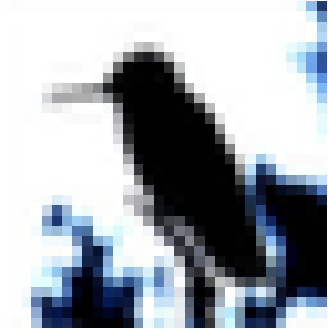
Using the optimization problem described in previous section, we compute the distance of testing samples from the $\mathcal{H}^{tr}$ , for the MNIST and CIFAR-10 datasets. Figure 1 shows the histogram of distances and Figure 2 shows samples of testing images that are farthest from their $\mathcal{H}^{tr}$ .

Refer to caption — (a) MNIST (pixel space)

To get a better sense of how far these distances are, consider the $\mathcal{H}^{tr}$ of CIFAR-10 dataset. Its diameter, the largest distance between any pair of vertices in $\mathcal{H}^{tr}$ , is 13,621 (measured by Frobenius norm in pixel space). On the other hand, the distance of farthest testing image from the $\mathcal{H}^{tr}$ is about 3,500 (about 27% of the diameter of $\mathcal{H}^{tr}$ ). Moreover, the average distance between pairs of images in the training set of CIFAR-10 is 4,838, while the closest pair of images are only 701 apart.

Hence, the distance of testing data to $\mathcal{H}^{tr}$ is not negligible and we cannot dismiss it as a small noise. However, it is not very large either. When we convolve the images with Haar or Daubechies (Daubechies, 1992) wavelets (an operation analogous to convolutions performed by CNNs), the testing samples still remain outside the $\mathcal{H}^{tr}$ in the wavelet space. When we choose a small subset of wavelet coefficients for all images, still, the testing samples remain outside the $\mathcal{H}^{tr}$ in that lower dimensional space, and the distances still resemble a normal distribution.

Overall, we can say that in order to classify most of the testing images in the above datasets, a model has to extrapolate, to some moderate degree, outside its $\mathcal{H}^{tr}$ . In Appendix A, we discuss the convex hull of random points in high-dimensional space and explain that the distance to convex hulls will be much larger if we deal with random points instead of these images. This signifies that training and testing sets of these datasets are related to each other, and the extent of extrapolation task is limited.

2.3 Directions to $\mathcal{H}^{tr}$ and the information they contain

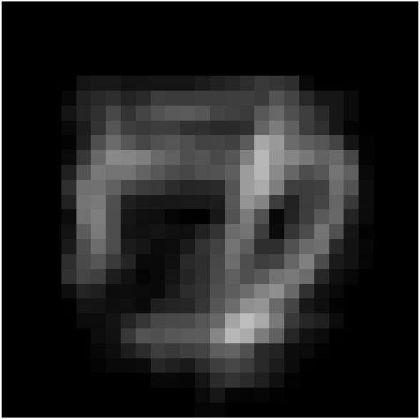
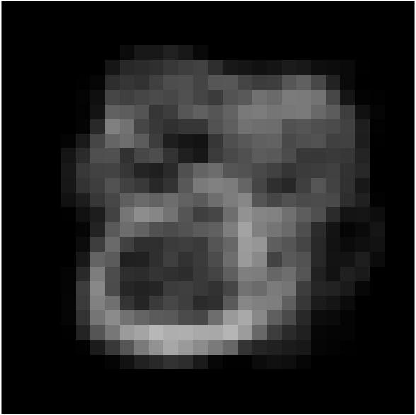
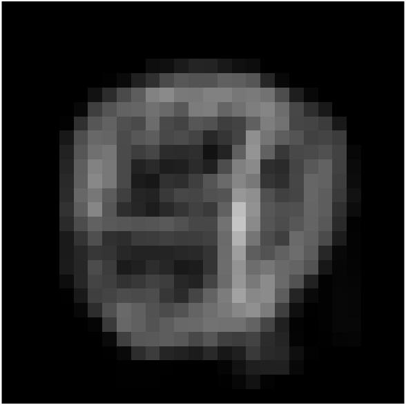
For each image that is outside the $\mathcal{H}^{tr}$ , there is some minimum perturbation that would bring that image to the $\mathcal{H}^{tr}$ . Figures 3 and 4 show that perturbation for some images in the testing set of CIFAR-10 and MNIST.

The perturbations required to bring testing images to the $\mathcal{H}^{tr}$ specifically relate to the objects of interest depicted in images and they appear to impact the images significantly. Therefore, the extrapolation required to classify those images can be considered significant, too.

If we merely choose the image in training set that is closest to the query image, the distance to the query image will be considerably larger and the differences between the two images will not be related to distinctive features. Figure 5 shows this for the image we considered in the first row of Figure 3, which is the very first testing image in the dataset. Hence, the interpolation performed between the training samples is useful in defining the extrapolation task.

(original) Refer to caption - = (closest image in $\mathcal{H}^{tr}$ )

Figure 5: The distance between an outside image and the closest image to it in the

\mathcal{H}^{tr}

can be considerably large, compared to the distance between the image and the boundary of

\mathcal{H}^{tr}

. The direction between the outside image and the closest image to it is usually unrelated to the distinctive features in images.

2.4 Images that form the surface closest to the outside image

The image on the surface of $\mathcal{H}^{tr}$ , closest to an image, $x^{te}$ , outside the $\mathcal{H}^{tr}$ , is a convex combination of some training images. We call those training images as the support for $x^{te}$ . In our experiments, the number of support images for each testing image is only a few. For example, the image on the second row of Figure 3 has only 26 support images in the training set. Figure 6 shows 10 of those 26 images with their corresponding coefficients in the convex combination.

$\xrightarrow[]{\mathcal{H}^{tr}}$ = 0.1129 + 0.1032 + 0.0878 + 0.0704

+ 0.0630 + 0.0536 + 0.0533 + 0.0529 + 0.0516

+ 0.0427 + $\dots$

Figure 6: Projection of a testing image to the

\mathcal{H}^{tr}

, and the convex combination of images in training set that create the projected image. There are 26 training images used in the convex combination, but we have shown 10 of those with the largest coefficients.

2.5 Internal representation of images learned by deep networks

The success of deep learning models is attributed to the features they extract from images before their final classification layer. Let’s consider a standard ResNet model (He et al., 2016) trained on the CIFAR-10 training set. The internal layer of network just before the last pooling layer has 4,096 dimensions. In that space, testing samples are outside the convex hull of training set, similar to the pixel space. Hence, all the operations and feature extractions performed on images, from pixel space all the way to the last pooling layer do not bring the testing samples inside the convex hull of training sets.

The last pooling layer then projects the images to a 64 dimensional space, and consequently to a 10-dimensional space which corresponds to the 10 output classes of network. Even in the 64-dimensional space, all testing images are outside the $\mathcal{H}^{tr}$ while their distances resemble a normal distribution as shown in Figure 7.

Figure 8 shows the testing images that are farthest from $\mathcal{H}^{tr}$ in that 64-dimensional representations of images.

Figure 8: The 5 testing images that are farthest from the

\mathcal{H}^{tr}

in the internal 64-dimensional space after the last pooling layer of a trained ResNet model. Compare these to farthest images from

\mathcal{H}^{tr}

in the pixel space as shown in Figure 2(b).

It may be speculated that there is a low dimensional manifold, learned by deep networks, where all (or most) testing samples are included in the convex hull of training set and the functional task of a deep network on that manifold is interpolation. We observed here that there is no trace of such manifold even in the internal representation of a trained ResNet. We saw that even in the 64-dimensional layer right before the classification layer, testing samples are outside the $\mathcal{H}^{tr}$ and their distance to $\mathcal{H}^{tr}$ is still significant.

In fact, in all the analysis presented we found no indication that the task of classifying testing images of our datasets can be considered an interpolation task.

2.6 Takeaways from geometric properties of datasets

We can conclude that with such number of training samples in such high-dimensional domains, one can expect the testing samples to be outside their $\mathcal{H}^{tr}$ . However, directions to the convex hulls are significant in size, and they contain information related to the objects of interest in images. By investigating the representation of images in internal layers of a standard ResNet model, we observed that testing images are outside the convex hull of training set, all along the layers of the network, even after the last pooling layer which only has 64-dimensions. All our analysis indicated that classifying images of these datasets is generally an extrapolation task (to a moderate degree).

Therefore, the generalization of over-parameterized image classifiers cannot be explained by mere interpolation. Instead, we have to consider interpolation in tandem with extrapolation. Interpolation defines the decision boundaries inside the $\mathcal{H}^{tr}$ and brings them to the surface of $\mathcal{H}^{tr}$ . Extrapolation helps us shape their extensions to some degree outside the $\mathcal{H}^{tr}$ .

When a human (even a young child) classifies the object in an image (e.g., a car), it is hard to imagine that they are interpolating between images of that object available in their memory. Even if we consider a very large training set of images of an object, it would be relatively easy to come up with a legitimate image of that object that falls outside the convex hull of that large training set.

It may be argued that location of decision boundaries are not important in the pixel space, but that would be ignoring the domain of our function. How can the domain not be important? Previous studies such as (Elsayed et al., 2018; Jiang et al., 2019) have shown that pushing the decision boundaries away from the training samples in the pixel space improves the generalization of models. Adversarial examples are also created in the pixel space and another line of research is trying to push the decision boundaries away from samples to make the models less vulnerable (Cohen et al., 2019). Therefore location of decision boundaries in the domain is actually what researchers have been using to understand and change the main functional traits of our deep networks. In fact, even basic training techniques such as mirroring training images (horizontally) and feeding them to the model as extra training samples, aim to define decision boundaries in more regions of the domain.

This is not to say that if we train a model to classify images of shoes, it can go on to extrapolate outside the scope of what it has learned, and classify the contents of any image, e.g., classify tumors in radiology images of liver. We do not use the “extrapolation” in that sense. When we studied the $\mathcal{H}^{tr}$ of random points (in Appendix A), we clearly saw that there is a close relationship between the training and testing sets of our image datasets, and we also know from the literature that there is an intimate relationship between the spatial location of decision boundaries of the models and their training and testing sets. Nevertheless, it is mathematically proper to say that the task of classifying unseen images can be an extrapolation task, outside the $\mathcal{H}^{tr}$ of what the model has seen/learned to some moderate degree.

To this end, we can consider 2 levels of extrapolation: 1- Extrapolating moderately outside the training set, but within the scope of training set, (moderate may be some fraction of the diameter of $\mathcal{H}^{tr}$ , for example) and 2- Extrapolating outside that scope. We use the term “extrapolation” in the former sense and not the latter.

The latter case relates to the out-of-distribution detection literature in deep learning. Understanding the distribution of image datasets has been a challenging task and we still do not have reliable tools to detect out-of-distribution images. For example, a model trained on CIFAR-10 may confidently classify an MNIST digit as a cat without even realizing that a handwritten digit has no similarity to what it has seen during training. Numerous papers have tried to address this shortcoming of deep networks, but it is still an open research problem. We believe considering the geometry of data may be useful in the out-of-distribution detection, too.

We have to remain mindful that in the pixel space, spatial locations and Euclidean distances are not always meaningful. For example, we can move considerable distances in the pixel space by changing the background of an image of a cat, or by changing the color of the cat, or by moving the cat from one location in the image to another location. Therefore, drawing an exact line as to which regions outside the $\mathcal{H}^{tr}$ should be considered out-of-distribution is not so easy. This also relates to recent empirical studies on the foreground/background effect of images on deep learning generalization (Xiao et al., 2020). We believe the geometric perspective we propose in this paper can be a useful guide for such studies.

The perspective we propose here remains consistent in all these subfields of the literature. When we train a model, we define its decision boundaries inside its $\mathcal{H}^{tr}$ , and those decision boundaries extend outside the $\mathcal{H}^{tr}$ all over the domain, even to areas where we do not have any training samples. By over-parameterization and training regimes, we manage to form the extensions of our decision boundaries to some extent outside the $\mathcal{H}^{tr}$ and that is our key to classifying testing images. Nevertheless, we do not have control over how decision boundaries extend to all regions outside the $\mathcal{H}^{tr}$ . For training a network, we gradually minimize the loss function of the model on training set, while observing how that minimization affects the accuracy of model on a validation set. Watching the validation set is our guide to shaping the extensions of decision boundaries while we train a model.

Our definition of extrapolation corresponds to the definition of generalization. In the literature, when one says a deep network generalizes to classify unseen images, they do not mean that it generalizes from classifying handwritten digits to classifying tumors in radiology images. They mean that the model generalizes to classify unseen images related to images that it has been trained on. We use the term extrapolation in that same sense.

For our purpose of studying generalization, we are concerned with how the extensions of decision boundaries are formed to some moderate degree outside its $\mathcal{H}^{tr}$ , and how it relates to over-parameterization, training regime, and accuracy of model on testing sets. We will explore them in the next section.

3 Learning outside the convex hull: A polynomial decision boundary

In the previous section, we showed that all testing samples of MNIST and CIFAR-10 are considerably outside the convex hull of their corresponding training sets, while the distance to the $\mathcal{H}^{tr}$ has noticeable variations, resembling a normal distribution. Hence, a trained deep learning model somehow manages to define its decision boundaries accurately enough outside the boundaries of what it has observed during training. But how does a model achieve that, or more precisely, how do we manage to train a model such that its decision boundaries have the desirable form outside the $\mathcal{H}^{tr}$ ?

Since we are interested in the generalization of image classifiers, and the pixel space is a bounded space, we consider the domain to be bounded, while the $\mathcal{H}^{tr}$ occupies some portion of it. Testing data can be inside and outside the $\mathcal{H}^{tr}$ , but always inside the bounded domain.

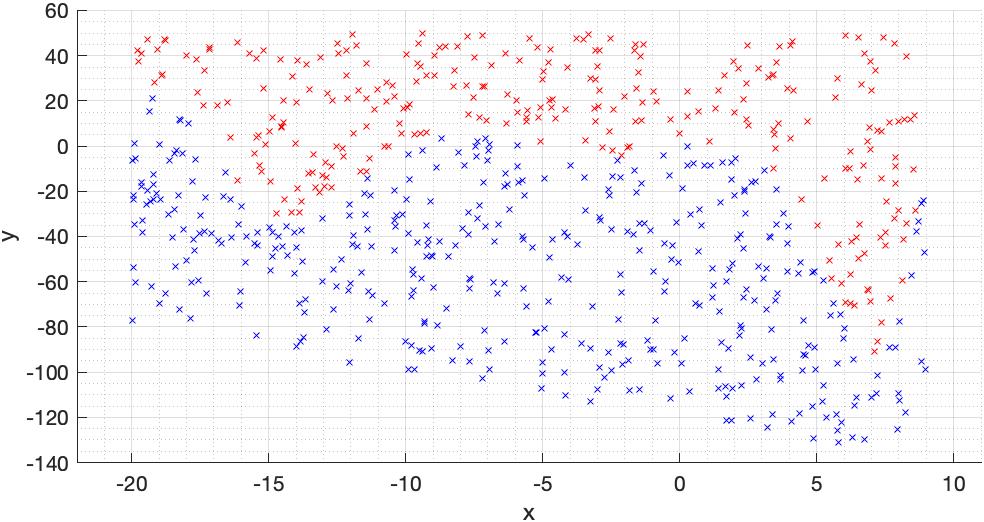
Let’s now use a polynomial decision boundary as an example to gain some intuitive insights.²²2Choosing a polynomial decision boundary is appropriate because many recent studies on deep learning generalization consider regression models that interpolate, e.g. (Belkin et al., 2018b, a, 2019; Liang et al., 2020; Verma et al., 2019; Kileel et al., 2019; Savarese et al., 2019). However, we note that those studies do not consider the convex hull of training sets. Figure 11(a) shows two point sets colored in blue and red, each set belonging to a class. These sets are non-linearly separable, because they have no overlap. If we use the polynomial

y=10^{-5}(x+20)(x+17)(x+10)(x+5)(x)(x-2)(x-9),

(5)

as our decision boundary, we achieve perfect accuracy in separating these two sets, as shown in Figure 11(b).

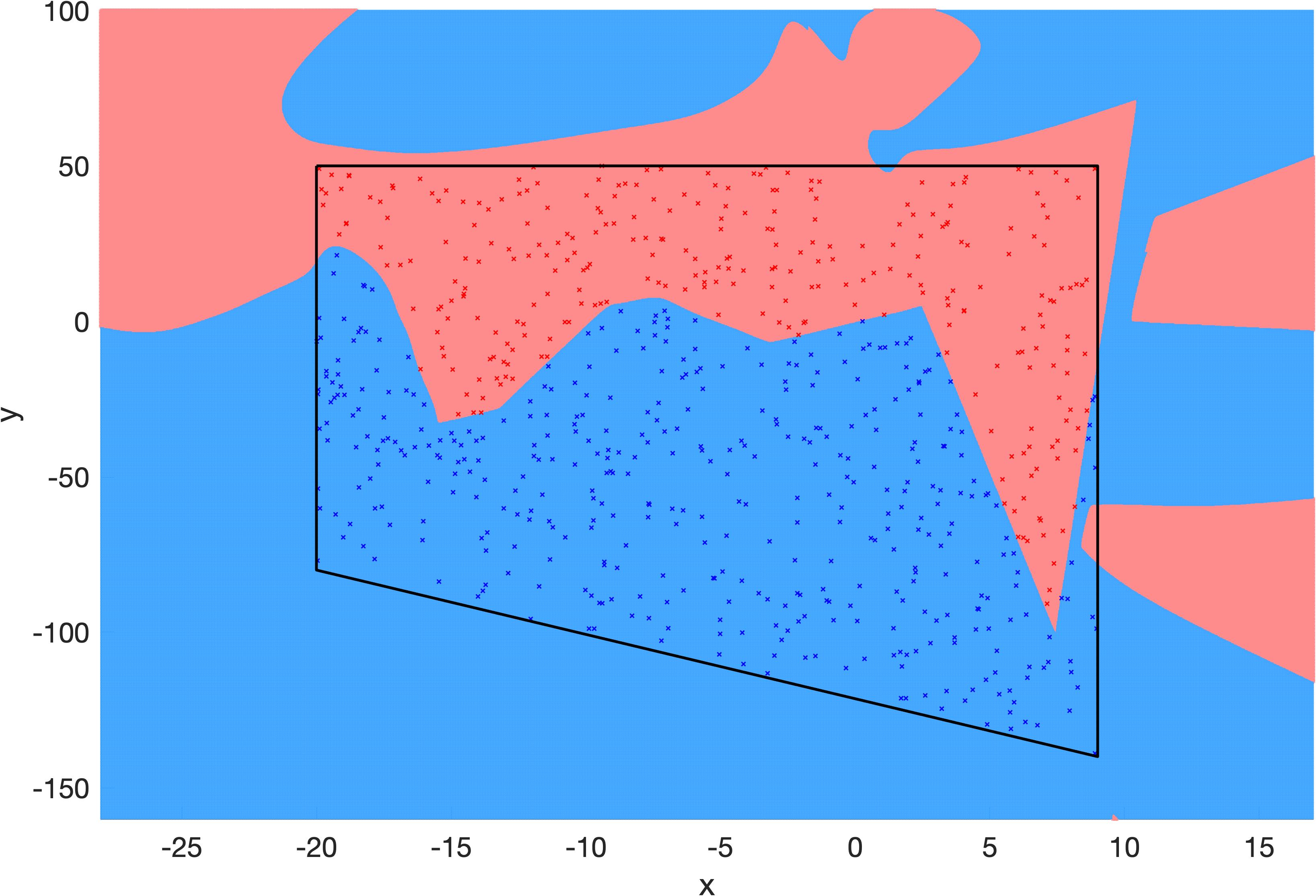
Now that we have obtained this polynomial, i.e., decision boundary, we would be interested to know how it generalizes to unseen data. Let’s assume that our bounded domain is defined by the limits shown in Figure 10 which also shows how our decision boundary generalizes outside the $\mathcal{H}^{tr}$ . If our polynomial can correctly separate and label our testing data, we would say that our polynomial is generalizing well, and vice versa. But, what is reasonable to expect from the testing data? In what regions of the domain should we be hopeful that our polynomial can generalize? What if the domain is much larger than the $\mathcal{H}^{tr}$ ? Is the extension of our polynomial on both sides reasonable enough?

Clearly, the answer to the above questions can be different inside and outside the $\mathcal{H}^{tr}$ . Inside the $\mathcal{H}^{tr}$ , if the unseen data has a similar label distribution as the training set, we can be hopeful that our decision boundary will generalize well. However, outside the $\mathcal{H}^{tr}$ is uncharted territory and hence, there will be less hope/confidence about the generalization of our decision boundary, especially when we go far outside the $\mathcal{H}^{tr}$ .

Now, let’s assume that from some prior knowledge, we know that the decision boundary in Figure 11 is the unique decision boundary that perfectly classifies the testing data. In such case, the decision boundary defined by equation (5) and shown in Figure 10 will generalize poorly outside the $\mathcal{H}^{tr}$ , despite the fact that it perfectly fits the training data.

How can we incorporate that prior knowledge into the decision boundary defined by equation (5) and reshape it to the decision boundary in Figure 11, so that it can generalize well both inside and outside the $\mathcal{H}^{tr}$ ? How can we change the shape of our polynomial outside the $\mathcal{H}^{tr}$ , while maintaining its current shape inside the $\mathcal{H}^{tr}$ ? Clearly, we should add to the degree of our polynomial, or in other words, we should over-parameterize it. The necessity of over-parameterization for achieving that goal for our polynomial decision boundary can be rigorously shown using the orthogonal system of Legendre polynomials (Ascher and Greif, 2011).

From this perspective, over-parameterization is necessary, but it is not sufficient for good generalization, because for an over-parameterized polynomial (i.e., decision boundary), there will be infinite number of solutions that can fit the training data, but each of them would have a different shape outside the $\mathcal{H}^{tr}$ . In fact, an over-parameterized polynomial can have the same shape as the polynomial in Figure 10. But, how can we pick the decision boundary that fits the data and also generalizes well outside the $\mathcal{H}^{tr}$ ?

In the over-parameterized regime, the key to finding the desirable decision boundary is the optimization process, i.e., the training regime. In other words, different training regimes would lead us to decision boundaries that all perfectly fit the training set, but each has a different shape outside the $\mathcal{H}^{tr}$ . This highlights that over-parameterization and training regime work in tandem to shape the extensions of our decision boundary. However, many studies consider them separately in the deep learning literature.

4 Output of deep learning functions outside their $\mathcal{H}^{tr}$

In this section, we investigate a 2-layer neural network with ReLU activation functions. We train the model with various number of neurons on the data from previous section as depicted in Figure 11(b). We then investigate the output of trained models inside and outside of the $\mathcal{H}^{tr}$ , as shown in Figures 12-14. In these figures, the black trapezoid depicts the $\mathcal{H}^{tr}$ . The colors red and blue correspond to our 2 classes.

Because of the non-convexity of the loss function, the loss may have numerous minimizers, however, when the model is under-parameterized, as in Figure 12, none of those minimizers would make the loss zero. Finding the same minimizer of training loss is equivalent to obtaining the same trained model, hence unlike the over-parameterized setting, the training regime is focused on finding the global minimizer of the training loss, i.e., finding the best shape for the decision boundary inside the convex hull.

As we increase the number of neurons with increments of 2, we see the model with 30 neurons can perfectly separate the 2 classes in our training set. Figure 13 shows the output of 3 different 30-neuron models that are trained with different training regimes.

Finally, we consider models that are highly over-parameterized. In this regime, there are infinite number of parameter configurations that minimize the training loss to zero, which is equivalent to developing the decision boundaries that perfectly separate our two classes.

The above observations explain why we need over-parameterized models for deep learning and why the generalization of deep learning models are so susceptible to different training regimes. Appendix B provides further discussion on this topic and a broader perspective on how interpolation and extrapolation complement each other.

5 Conclusion and future work

We showed that all testing data for standard image classification models considerably lie outside the convex hull of their training sets, in pixel space, in wavelet space, and in the internal representations learned by deep networks. Therefore, the generalization of a deep network relies on its capability to extrapolate outside the boundaries of the data it has seen during training. Based on this observation, the significant number of studies that focus on interpolation regimes seem to be inadequate in explaining the generalization of deep networks.

From this perspective, over-parameterization of models may be considered a necessity to desirably form the extension of decision boundaries outside the convex hull of data. This can be proven for polynomial regression models using the orthogonal system of Legendre polynomials. Moreover, we showed that the training regime can significantly affect the shape of decision boundaries outside the convex hulls, affecting the accuracy of a model in its extrapolation. We investigated a 2-layer ReLU network and a polynomial decision boundary to demonstrate these ideas.

This work opens an avenue to study deep learning models from a new geometric perspective. As we explained earlier, most of the literature on deep learning generalization and their functional behavior is focused on interpolation models and interpolation assumptions. Many studies in the past few years have explicitly used mere interpolation to explain how deep networks learn to classify images and why they need so many parameters. Most notable examples of such studies are (Belkin et al., 2019; Ma et al., 2018; Belkin et al., 2018b). Our findings would encourage those studies to broaden their geometric perspective and consider extrapolation in tandem with interpolation in order to explain the generalization in deep learning.

————

Acknowledgments

R.Y. thanks Tammy Kolda for helpful discussion and Shai Shalev-Shwartz for a helpful comment. R.Y. also thanks Yaim Cooper for the discussion that led to Appendix A, and thanks Benjamin Raichel for helpful pointer to approximation algorithms for convex hulls. R.Y. was supported by a fellowship from the Department of Veteran Affairs. The views expressed in this manuscript are those of the author and do not necessarily reflect the position or policy of the Department of Veterans Affairs or the United States government.

References

Arora et al. (2019) Sanjeev Arora, Nadav Cohen, Wei Hu, and Yuping Luo. Implicit regularization in deep matrix factorization. In Advances in Neural Information Processing Systems, pages 7413–7424, 2019.
Ascher and Greif (2011) Uri M Ascher and Chen Greif. A first course on numerical methods. SIAM, 2011.
Barnard and Wessels (1992) Etienne Barnard and LFA Wessels. Extrapolation and interpolation in neural network classifiers. IEEE Control Systems Magazine, 12(5):50–53, 1992.
Belkin et al. (2018a) Mikhail Belkin, Daniel J Hsu, and Partha Mitra. Overfitting or perfect fitting? Risk bounds for classification and regression rules that interpolate. In Advances in neural information processing systems, pages 2300–2311, 2018a.
Belkin et al. (2018b) Mikhail Belkin, Siyuan Ma, and Soumik Mandal. To understand deep learning we need to understand kernel learning. In International Conference on Machine Learning, pages 541–549, 2018b.
Belkin et al. (2019) Mikhail Belkin, Daniel Hsu, Siyuan Ma, and Soumik Mandal. Reconciling modern machine-learning practice and the classical bias–variance trade-off. Proceedings of the National Academy of Sciences, 116(32):15849–15854, 2019.
Blum et al. (2019) Avrim Blum, Sariel Har-Peled, and Benjamin Raichel. Sparse approximation via generating point sets. ACM Transactions on Algorithms (TALG), 15(3):1–16, 2019.
Cohen et al. (2019) Jeremy Cohen, Elan Rosenfeld, and Zico Kolter. Certified adversarial robustness via randomized smoothing. In International Conference on Machine Learning, pages 1310–1320, 2019.
Cohen et al. (2020) Uri Cohen, SueYeon Chung, Daniel D Lee, and Haim Sompolinsky. Separability and geometry of object manifolds in deep neural networks. Nature communications, 11(1):1–13, 2020.
Cooper (2018) Yaim Cooper. The loss landscape of overparameterized neural networks. arXiv preprint arXiv:1804.10200, 2018.
Daubechies (1992) Ingrid Daubechies. Ten Lectures on Wavelets. Society for Industrial and Applied Mathematics, Philadelphia, 1992.
Ellis et al. (2018) Kevin Ellis, Daniel Ritchie, Armando Solar-Lezama, and Josh Tenenbaum. Learning to infer graphics programs from hand-drawn images. In Advances in neural information processing systems, pages 6059–6068, 2018.
Elsayed et al. (2018) Gamaleldin Elsayed, Dilip Krishnan, Hossein Mobahi, Kevin Regan, and Samy Bengio. Large margin deep networks for classification. In Advances in Neural Information Processing Systems, pages 842–852, 2018.
Fawzi et al. (2018) Alhussein Fawzi, Seyed-Mohsen Moosavi-Dezfooli, Pascal Frossard, and Stefano Soatto. Empirical study of the topology and geometry of deep networks. In Proceedings of the IEEE Conference on Computer Vision and Pattern Recognition, pages 3762–3770, 2018.
Fink et al. (2016) Martin Fink, John Hershberger, Nirman Kumar, and Subhash Suri. Hyperplane separability and convexity of probabilistic point sets. In 32nd International Symposium on Computational Geometry (SoCG 2016). Schloss Dagstuhl-Leibniz-Zentrum fuer Informatik, 2016.
Goldstein et al. (2015) Tom Goldstein, Min Li, and Xiaoming Yuan. Adaptive primal-dual splitting methods for statistical learning and image processing. In Advances in Neural Information Processing Systems, pages 2089–2097, 2015.
Haffner (2002) Patrick Haffner. Escaping the convex hull with extrapolated vector machines. In Advances in Neural Information Processing Systems, pages 753–760, 2002.
He et al. (2016) Kaiming He, Xiangyu Zhang, Shaoqing Ren, and Jian Sun. Deep residual learning for image recognition. In Proceedings of the IEEE conference on computer vision and pattern recognition, pages 770–778, 2016.
Hueter (1999) Irene Hueter. Limit theorems for the convex hull of random points in higher dimensions. Transactions of the American Mathematical Society, 351(11):4337–4363, 1999.
Jiang et al. (2019) Yiding Jiang, Dilip Krishnan, Hossein Mobahi, and Samy Bengio. Predicting the generalization gap in deep networks with margin distributions. In International Conference on Learning Representations, 2019.
Kanbak et al. (2018) Can Kanbak, Seyed-Mohsen Moosavi-Dezfooli, and Pascal Frossard. Geometric robustness of deep networks: Analysis and improvement. In Proceedings of the IEEE Conference on Computer Vision and Pattern Recognition, pages 4441–4449, 2018.
Kileel et al. (2019) Joe Kileel, Matthew Trager, and Joan Bruna. On the expressive power of deep polynomial neural networks. In Advances in Neural Information Processing Systems, pages 10310–10319, 2019.
Kosanovich et al. (1996) K Kosanovich, A Gurumoorthy, E Sinzinger, and M Piovoso. Improving the extrapolation capability of neural networks. In Proceedings of the 1996 IEEE International Symposium on Intelligent Control, pages 390–395. IEEE, 1996.
Krizhevsky (2009) Alex Krizhevsky. Learning multiple layers of features from tiny images. 2009.
LeCun et al. (1998) Yann LeCun, Léon Bottou, Yoshua Bengio, and Patrick Haffner. Gradient-based learning applied to document recognition. Proceedings of the IEEE, 86(11):2278–2324, 1998.
Liang et al. (2020) Tengyuan Liang, Alexander Rakhlin, et al. Just interpolate: Kernel “ridgeless” regression can generalize. Annals of Statistics, 48(3):1329–1347, 2020.
Ma et al. (2018) Siyuan Ma, Raef Bassily, and Mikhail Belkin. The power of interpolation: Understanding the effectiveness of sgd in modern over-parametrized learning. In International Conference on Machine Learning, pages 3325–3334. PMLR, 2018.
Neyshabur et al. (2017a) Behnam Neyshabur, Srinadh Bhojanapalli, David McAllester, and Nati Srebro. Exploring generalization in deep learning. In Advances in Neural Information Processing Systems, pages 5947–5956, 2017a.
Neyshabur et al. (2017b) Behnam Neyshabur, Ryota Tomioka, Ruslan Salakhutdinov, and Nathan Srebro. Geometry of optimization and implicit regularization in deep learning. arXiv preprint arXiv:1705.03071, 2017b.
Neyshabur et al. (2019) Behnam Neyshabur, Zhiyuan Li, Srinadh Bhojanapalli, Yann LeCun, and Nathan Srebro. Towards understanding the role of over-parametrization in generalization of neural networks. In International Conference on Learning Representations, 2019.
Nocedal and Wright (2006) Jorge Nocedal and Stephen Wright. Numerical Optimization. Springer, New York, 2nd edition, 2006. ISBN 9780387400655.
O’Leary and Rust (2013) Dianne P O’Leary and Bert W Rust. Variable projection for nonlinear least squares problems. Computational Optimization and Applications, 54(3):579–593, 2013.
Papernot et al. (2016) Nicolas Papernot, Patrick McDaniel, Somesh Jha, Matt Fredrikson, Z Berkay Celik, and Ananthram Swami. The limitations of deep learning in adversarial settings. In IEEE European symposium on security and privacy (EuroS&P), pages 372–387. IEEE, 2016.
Psichogios and Ungar (1992) Dimitris C Psichogios and Lyle H Ungar. A hybrid neural network-first principles approach to process modeling. AIChE Journal, 38(10):1499–1511, 1992.
Savarese et al. (2019) Pedro Savarese, Itay Evron, Daniel Soudry, and Nathan Srebro. How do infinite width bounded norm networks look in function space? In Conference on Learning Theory, pages 2667–2690, 2019.
Shafahi et al. (2019) Ali Shafahi, W Ronny Huang, Christoph Studer, Soheil Feizi, and Tom Goldstein. Are adversarial examples inevitable? In International Conference on Learning Representations, 2019.
Snell et al. (2017) Jake Snell, Kevin Swersky, and Richard Zemel. Prototypical networks for few-shot learning. In NeurIPS, pages 4077–4087, 2017.
Strang (2019) Gilbert Strang. Linear Algebra and Learning from Data. Wellesley-Cambridge Press, 2019.
Tsipras et al. (2019) Dimitris Tsipras, Shibani Santurkar, Logan Engstrom, Alexander Turner, and Aleksander Madry. Robustness may be at odds with accuracy. In International Conference on Learning Representations, 2019.
Verma et al. (2019) Vikas Verma, Alex Lamb, Christopher Beckham, Amir Najafi, Ioannis Mitliagkas, David Lopez-Paz, and Yoshua Bengio. Manifold mixup: Better representations by interpolating hidden states. In International Conference on Machine Learning, pages 6438–6447. PMLR, 2019.
Vincent and Bengio (2002) Pascal Vincent and Yoshua Bengio. K-local hyperplane and convex distance nearest neighbor algorithms. In Advances in neural information processing systems, pages 985–992, 2002.
Xiao et al. (2020) Kai Xiao, Logan Engstrom, Andrew Ilyas, and Aleksander Madry. Noise or signal: The role of image backgrounds in object recognition. arXiv preprint arXiv:2006.09994, 2020.
Xu et al. (2020) Keyulu Xu, Jingling Li, Mozhi Zhang, Simon S Du, Ken-ichi Kawarabayashi, and Stefanie Jegelka. How neural networks extrapolate: From feedforward to graph neural networks. arXiv preprint arXiv:2009.11848, 2020.
Yousefzadeh and Huang (2020) Roozbeh Yousefzadeh and Furong Huang. Using wavelets and spectral methods to study patterns in image-classification datasets. arXiv preprint arXiv:2006.09879, 2020.
Zhang et al. (2017) Chiyuan Zhang, Samy Bengio, Moritz Hardt, Benjamin Recht, and Oriol Vinyals. Understanding deep learning requires rethinking generalization. In International Conference on Learning Representations, 2017.

A The case of random data in high-dimensional space

The question may arise that what happens if we have random data points in the same high-dimensional space. Would the data points still fall outside the $\mathcal{H}^{tr}$ ? Would the distance to $\mathcal{H}^{tr}$ be the same? The answers are yes and no, respectively.

To gain some insights, let’s consider the CIFAR-10 dataset. We can randomly shuffle all the pixel values in all the images of training and testing sets. In such case, the shuffled testing data would still fall outside the $\mathcal{H}^{tr}$ of shuffled data. But, their distance to $\mathcal{H}^{tr}$ would be orders of magnitude larger.

Alternatively, when we generate random points in the same domain as the pixel space of CIFAR-10, (i.e., domain with 3,072 dimensions bounded between 0 and 255), again, the testing data are outside the $\mathcal{H}^{tr}$ .³³3This relates to the limit theorems for the convex hull of random points in higher dimensions (Hueter, 1999) and also to studies on separability and distribution of random points (Fink et al., 2016). This time, the distances to $\mathcal{H}^{tr}$ are much larger even compared to the case of shuffling the pixel values.

We can conclude that with such number of training samples in such high-dimensional domains, one can expect the testing samples to be outside their $\mathcal{H}^{tr}$ . However, the distance to the convex hulls are much closer for our image datasets, compared to random data points, because for each testing image, $x^{te}$ , there are a group of training images that form a surface on the $\mathcal{H}^{tr}$ , and that surface is much closer to $x^{te}$ , compared to the surface that a set of random data points can create.

As we showed earlier, the directions to $\mathcal{H}^{tr}$ contain information about the objects of interest depicted in images. Hence, the extrapolation task of a neural network is meaningful and related to what it needs to classify in images. Recently, there has been further studies that try to learn images from even fewer training samples, i.e., few-shot learning (Snell et al., 2017), which implies a more advanced extrapolation task. This is also pursued by recent studies in cognitive science (Ellis et al., 2018).

B Extrapolation and interpolation work in tandem

Earlier, we reported that the extent of extrapolation, for the CIFAR-10 dataset, is about 27% of the diameter of its $\mathcal{H}^{tr}$ . We also reported that all testing samples are outside the $\mathcal{H}^{tr}$ . Based on these observations, we can say that the task of classifying the testing set of CIFAR-10 is extrapolation. But, how does the interpolation affect our ability to extrapolate? We can explain this using the decision boundaries of the models.

For image classification, our domain is a $d$ -dimensional hyper-cube, because pixel values are bounded. $d$ is the number of pixels. The convex hull of training set, $\mathcal{H}^{tr}$ , is a shape with $\leq d$ dimension, and sits somewhere in that hyper-cube. For CIFAR-10 dataset, $\mathcal{H}^{tr}$ has exactly $d$ dimensions. The testing samples sit around the $\mathcal{H}^{tr}$ , like a mist, not too far, and not too close to $\mathcal{H}^{tr}$ . The distance of testing samples from $\mathcal{H}^{tr}$ ranges between 1%-27% of its diameter, with average value of 10%.

As we mentioned earlier, a classification function/model partitions its domain and assigns a class to each of the partitions. The partitions are defined by decision boundaries, and so is the model. Basically, the training process partitions the shape $\mathcal{H}^{tr}$ by defining a finite set of decision boundaries inside it. We can define this process as interpolation, especially if we are only concerned about the location of decision boundaries in $\mathcal{H}^{tr}$ . Some of the decision boundaries defined in this process will reach the surface of $\mathcal{H}^{tr}$ and extend outside it. Theses decision boundaries and their extensions outside the hull are the ones that a model relies upon in order to classify the images outside the hull.

Because the testing images are not too far outside the hull, the space to shape the extensions of decision boundaries is limited. Therefore, the locations where the decision boundaries reach the surface of $\mathcal{H}^{tr}$ is of great importance. Overall, interpolation and extrapolation work in tandem to shape the decision boundaries and the functional performance of image classification models.

Going back to the hyper-cube, during the training, the shape of $\mathcal{H}^{tr}$ is partitioned with some nonlinear surfaces (decision boundaries), and some of those surfaces extend outside the $\mathcal{H}^{tr}$ . The locations where the decision boundaries reach the surface of $\mathcal{H}^{tr}$ and their extension outside the $\mathcal{H}^{tr}$ is critical in how the model classifies the testing images that are sitting around the $\mathcal{H}^{tr}$ .

Deep Learning Generalization and the Convex Hull of Training Sets