Deep learning for intermittent gravitational wave signals
Abstract
The ensemble of unresolved compact binary coalescences is a promising source of the stochastic gravitational wave (GW) background. For stellar-mass black hole binaries, the astrophysical stochastic GW background is expected to exhibit non-Gaussianity due to their intermittent features. We investigate the application of deep learning to detect such non-Gaussian stochastic GW background and demonstrate it with the toy model employed in Drasco & Flanagan (2003), in which each burst is described by a single peak concentrated at a time bin. For the detection problem, we compare three neural networks with different structures: a shallower convolutional neural network (CNN), a deeper CNN, and a residual network. We show that the residual network can achieve comparable sensitivity as the conventional non-Gaussian statistic for signals with the astrophysical duty cycle of . Furthermore, we apply deep learning for parameter estimation with two approaches, in which the neural network (1) directly provides the duty cycle and the signal-to-noise ratio (SNR) and (2) classifies the data into four classes depending on the duty cycle value. This is the first step of a deep learning application for detecting a non-Gaussian stochastic GW background and extracting information on the astrophysical duty cycle.
I Introduction
The astrophysical stochastic gravitational-wave (GW) background is one of the most interesting targets for current and future GW experiments. It originates from the ensemble of many unresolved GW sources at high redshift and contains information about the mass function and redshift distribution of the sources.
Observations of binary black holes (BBH) and binary neutron stars (BNS) indicate that distant merger events could be detected as a stochastic GW background by the near-future ground-based detector network [1, 2, 3]. An estimation from the merger rate shows that the energy density of the background spectra of BBH- and BNS-origins would be similar, but the statistical behavior could be very different [2]. While sub-threshold BNS events typically overlap and create an approximately continuous background, the time interval between BBH events is much longer than the duration of the individual signal, and they do not overlap. Because of this, the BBH background could be highly non-stationary and non-Gaussian (sometimes referred to as intermittent or popcorn signal). The information on the non-Gaussianity could be used to disentangle the different origins of the GW sources [4].
Detection strategies for such non-Gaussian backgrounds have been discussed in the literature. First, Drasco & Flanagan [5] (DF03) derived the maximum likelihood detection statistic for the case of co-located, co-aligned interferometers characterized by stationary, Gaussian white noise with the burst-like non-Gaussian signals. Although the computational cost is significantly larger than the standard cross-correlation method, it has been shown that the maximum likelihood method can outperform the standard cross-correlation search. Subsequently, Thrane [6] presented a method that can be applied in the more realistic case of spatially separated interferometers with colored, non-Gaussian noise. Martellini & Regimbau [7, 8] proposed semiparametric maximum likelihood estimators. While they are framed in the context of frequentist statistics, Cornish & Romano [9] discussed the use of Bayesian model selection. Alternative methods were also discussed. Seto [10, 11] presented the use of the fourth-order correlation between four detectors. Smith & Thrane [12, 13] proposed a method to use sub-threshold BBHs in the matched-filtering search and demonstrated a Bayesian parameter estimation. Subsequently, Biscoveanu et al. [14] simulated the Bayesian parameter estimation of the primordial background (stationary, Gaussian) in the presence of an astrophysical foreground (non-stationary, non-Gaussian). Finally, Matas & Romano [15] showed that the hybrid frequentist Bayesian analysis is equivalent to a fully Bayesian approach and claimed that their method can be extended to non-stationary GW background. See also Ref. [16] for a comprehensive review.
In the general context of GW data analysis, the application of deep learning has been actively studied in the last five years. George & Huerta [17, 18] showed that deep neural networks can achieve a sensitivity comparable to the matched filtering for detection and parameter estimation of BBH mergers. Although their neural network does not predict the statistical error, several authors proposed a method to predict the posterior distributions [19, 20, 21, 22, 23]. Also, deep learning has been widely applied for various types of signal (e.g., BBH mergers [24, 25, 26], black hole ringdown GWs [27, 28, 29, 30], continuous GWs [31, 32, 33, 34, 35], supernovae [36], and hyperbolic encounters [37]).
In this work, we use deep learning to analyze a non-Gaussian GW background. The great advantage of deep learning is that it is computationally cheaper than the matched-filter-based approach. It is because neural networks learn the features of the data through a training process before being applied to real data. The data analysis of a stochastic background is usually performed by dividing the long-duration data stream (years) into short time segments (typically seconds; see e.g. [3]). If we want to apply the non-Gaussian statistic of DF03, it will take a much longer time to analyze each segment compared to the standard cross-correlation statistic. On the other hand, in the case of deep learning, once the training is completed, it can quickly analyze each segment and repeat the same analysis for a large number of data segments with similar feature of training data. In this way, it is expected to reduce the total time for the analysis. Another advantage is that neural networks can extract the features which are difficult to model. Thus, it could be applied to various types of non-Gaussian GW backgrounds even if the source waveform is not understood well. As a first step, we employ the toy model and the detection method proposed by DF03. We train the neural network with the dataset that is generated by the toy model and assess the neural network’s performance by comparing it with their detection method.
Finally, let us mention the work by Utina et al. [38], which has a similar purpose and developed neural network algorithms to detect the GW background from binary black hole mergers. In [38], the data is split into or second segments, and the neural network is trained with the injection of binary black hole events. On the other hand, our method is based on the toy model in DF03, which does not rely on a particular burst model and is designed to analyze segments with longer duration (as long as the computational power allows). In addition, we discuss the estimation of the intermittency (astrophysical duty cycle), while Utina et al. focused on the detection problem.
The paper is structured as follows. In Sec. II, we describe the signal model and the non-Gaussian statistic proposed by DF03, which is demonstrated for the comparison in the result sections. Section. III is dedicated to a review of deep learning algorithms used in this paper. Then, we show the results of the detection problem in Sec. IV and parameter estimation in Sec. V. Finally, we summarize our work in Sec. VI.
II Signal model and maximum likelihood statistic
II.1 signal model
We use a simple toy model used in DF03. The assumptions are the followings: two detectors that are co-located and co-aligned; the detector noises are white, stationary, Gaussian, and statistically independent; each astrophysical burst is represented by a sharp peak that has support only on a discretized time grid. The methodology could be easily extended to the case of spatially separated interferometers by introducing the overlap reduction function [39, 6]. Detector noise, in reality, is colored and highly non-Gaussian, non-stationary, and these effects should be taken into account before applying our method to the real data. In this paper, however, we focus on presenting the basic methodology of deep learning and the comparison with the DF03’s results. The assumption on the sharp peak signal is valid if the duration of the burst is shorter than the time resolution of the detector. In that case, the observed GW strain at the burst arrival time is the averaged amplitude over the time interval between the sampled time step. However, this assumption cannot be applied to the expected astrophysical backgrounds from BBHs and BNSs, and again, we leave it as future work.

A strain data obtained by each detector is denoted by , where labels the different detectors, and is a time index. We use to denote the GW signal. Including detector noise data, which is denoted by , we can express the strain data of the th detector as
| (1) |
The detector noise is randomly generated from Gaussian distribution, that is,
| (2) |
is a one-dimensional Gaussian distribution with a mean and a variance , i.e.,
| (3) |
Due to the assumption of stationarity and white, the variance is constant in time. We also assume that two detectors have noise with the same variance, and we set
| (4) |
throughout this paper.
Assuming that the GW burst rate is not so high that the bursts do not overlap, we model the probability density function of the strain value at time as
| (5) |
where is the variance of the amplitude of the bursts, and is so-called the (astrophysical) duty cycle. The duty cycle describes the probability that a burst is present in the detector at any chosen time and takes a value in the range of . The case of is equivalent to Gaussian stochastic GWs. On the other hand, it is reduced to the absence of the signal for . A signal exhibits non-Gaussianity as decreases. Figure 1 shows an example of the time-series signal generated based on Eq. (5). Following DF03, we define the signal-to-noise ratio (SNR) of the non-Gaussian stochastic background by
| (6) |
and use it for describing the strength of the signal.
II.2 Non-Gaussian statistic
As proposed in DF03, the likelihood ratio can be used as a detection statistic. Under the assumption of the noise model Eq. (2) and the signal model Eq. (5), the likelihood ratio can be reduced to
| (7) |
where
| (8) |
and
| (9) |
More details of the non-Gaussian statistic are described in Appendix A.
In the later section, we compare the results of the non-Gaussian statistic and the neural networks for the detection problem. As seen in Eq. (7), we need to perform the parameter space search to find the maximum value of in the four-dimensional space. To do that, we take the grid points spanning over the ranges of , , and with the regular interval of , , and .
III Basics of neural network
III.1 Structure
The fundamental unit of a neural network is called a(n) (artificial) neuron which is an artificial model of a nerve cell in a brain. A neuron takes values signaled by other neurons as inputs and returns a single value as an output. The alignment of neurons is called a layer, and a neural network consists of a sequence of layers. Each layer takes the output of the previous layer and passes its own output to the next layer. The input data of a neural network go through many layers, and a neural network returns the output data. In the following, we denote an input vector and an output vector of each layer by and , respectively. The dimensions of the input and the output depend on the type of layer, which is described below.
A fully connected layer is one of the fundamental layers of a neural network. It takes a one-dimensional real-valued vector as an input and returns a linear transformation of the input data. The operation can be described as
| (10) |
where is the number of elements of the input vector. The 0th component is set to be and represents the constant term of the linear transformation. The coefficients are called weight, and we must appropriately tune them before applying the neural network to real data.
A linear transformation like a fully connected layer is usually followed by a nonlinear function which is called an activation function. Most activation functions have no tunable parameters. In this work, we used a rectified linear unit (ReLU) defined by
| (11) |
An activation function can take input with arbitrary size and be applied elementwise.
For image recognition, it is important to capture the local pattern. To do so, filters with a much smaller size than that of the input data are used. A convolutional layer carries out a convolution between input data and filters. A neural network containing one or more convolutional layers is often called a convolutional neural network (CNN). In this work, we use a one-dimensional convolutional layer. It can take a two-dimensional tensor as an input that is denoted by . This represents the situation where each grid of the data has multiple values. The different values contained in one pixel are called channels, which are represented by the first index . For example, a color image has three channels corresponding to the primary colors, namely, red, blue, and green. In our case, the strain data has two channels corresponding to two different detectors. The second index corresponds to a pixel. Formally, we can write a one-dimensional convolutional layer by
| (12) |
where the parameter characterize the filter, is the filter size, and is the number of channels. The filter is applied multiple times to the input data by sliding it over the whole matrix. The parameter is called stride and controls the step width of the slide.
A pooling layer reduces the size of data by contracting several data points into one data point. There are several variants of pooling layers depending on how to reduce information. In the present work, we use two types of pooling. The max pooling layer is defined by
| (13) |
Also, we use the average pooling that is defined by,
| (14) |
The last layer of a neural network is called the output layer. It should be tailored depending on the problem to solve. For the regression, the identity function
| (15) |
is often applied. Usually, the identity function is not explicitly applied because it is trivial. On the other hand, the classification problem requires a more tricky layer. In the classification problem, the neural network is constructed in a way that each element of the output corresponds to the probability that the input is likely to belong to each class. To interpret the output as the probabilities, they must satisfy the following relations,
| (16) |
and
| (17) |
Here, is the number of target classes. A softmax layer that is defined by
| (18) |
is suitable for the classification problem. The output of a softmax layer (18) satisfies the conditions Eqs. (16) and (17).
III.2 Residual block
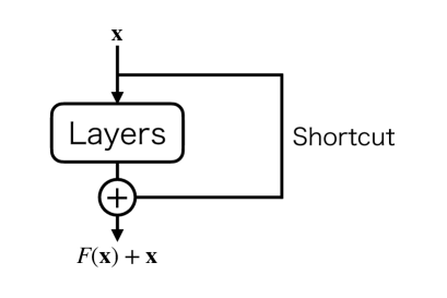
One may naively expect that a deeper neural network shows better performance. This expectation is valid to some extent. However, it is empirically known that the performance gets saturated as the network depth increases. On the contrary, the accuracy gets worse. It is known as the degradation problem. He et al. [40] proposed the residual learning to address the degradation problem. The idea of the residual network is to introduce a shortcut connection, as shown in Fig. 2, which enables us to efficiently train deep neural networks.

Figure 3 shows another type of residual block called a bottleneck block [40]. The main path has three convolutional layers. The first convolutional layer has a kernel size of one and reduces the number of channels. The second convolutional layer plays a role as a usual one. The third convolutional layer has a kernel size of 1 and recovers the number of channels. Both the first and the second convolutional layers are followed by ReLU activation (11). The batch normalization [41] is located at the end of the main path, where the average and the variance of the input data are calculated elementwise over the batch,
| (19) | ||||
| (20) |
Here, a batch is a subset of the training data, and is the size of a batch. The use of a batch in the training is explained in the later subsection, Sec. III.4. Using Eqs. (19) and (20), the batch normalization transforms the input data into
| (21) | ||||
| (22) |
where and are trainable parameters, the asterisk represents an elementwise multiplication, and is introduced to prevent the overflow. We set .
The shortcut connection also has a convolutional layer with a kernel size of one and a stride of two. The input data is reshaped to match the size of the output of the main path.
III.3 Supervised learning
Before applying the neural network to real data, we optimize the neural network’s weights using a dataset prepared in advance. The optimization process is called training. To train a neural network, we prepare a dataset consisting of many pairs of input data and target data, which is hereafter denoted by . In this paper, the input data is the time-series strain data, and the target data should be chosen appropriately depending on the problem to solve.
In this work, we treat two types of problems: regression and classification. For the regression problem, the injected values of the parameters can be used as the target values. For the classification problem in which the inputs are classified into several classes, the one-hot representation is widely used for the target vector. When the number of the target classes is , the target vector is a -dimensional vector that takes 0 or 1 for each element. If the input is assigned to the th class, only th element takes 1, and others are 0. For example, in the detection problem presented in Sec. IV, we have two classes, that is, the absence and the presence of the GW signal. In this case, the target vector is chosen as
| (23) |
In Sec. V, we demonstrate estimation of the duty cycle. We first apply the ordinary parameter estimation approach; the injected values of the parameters (the signal amplitude and the duty cycle) are used as the target values. In the second approach, we reduce the parameter estimation to the classification problem, in which the inputs are classified into four classes of duty cycle values.
III.4 Training process
In the training process, we use a loss function to quantify the deviation between the neural network predictions and the target values. For the regression, various choice exists. In this work, we employ the L1 loss defined by
| (24) |
where is the number of parameters to be estimated. For the classification problem, a cross-entropy loss, defined by,
| (25) |
is widely used.
The weights of a neural network are updated so that the sum of the loss functions for all training data is small. However, in general, the minimization of the loss function cannot be done analytically. Thus, the iterative process is employed. We divide the training data into several subsets, called a batch. In each step of the iteration, the prediction and the loss evaluation are made for all data contained in a given batch. The update process depends on the gradient of the sum of the loss function over the batch, i.e.,
| (26) |
where and are the prediction of the neural network and the target vector for the th data, respectively.
The simplest update procedure is the stochastic gradient descent method (SGD). In SGD, the derivatives of the loss function with respect to the neural network’s weights are calculated, and the weights are updated by the procedure
| (27) |
where we omit all subscripts and superscripts of just for brevity. is called learning rate and characterizes how much the update of weights is sensitive to the loss function gradients. A batch is randomly chosen for every iteration step. Many updated procedures have been proposed so far. Most of them commonly exploit the gradients of the loss function with respect to the weights. In spite of the tremendous number of the weights, the algorithm called back propagation enables us to efficiently calculate all gradients of the loss function.
IV Detection of non-Gaussian stochastic GWs
In this section, we present the application of deep learning to the detection problem of the non-Gaussian stochastic GW background.
IV.1 Setup of neural networks
| Layer | Output size | No. of parameters |
|---|---|---|
| Input | (2, 10000) | - |
| 1D convolutional | (16, 9993) | 272 |
| ReLU | (16, 9993) | - |
| 1D max pooling | (16, 2498) | - |
| 1D convolutional | (32, 2491) | 4128 |
| ReLU | (32, 2491) | - |
| 1D max pooling | (32, 622) | - |
| 1D convolutional | (64, 619) | 8256 |
| ReLU | (64, 619) | - |
| 1D max pooling | (64, 154) | - |
| 1D convolutional | (128, 151) | 32896 |
| ReLU | (128, 151) | - |
| 1D max pooling | (128, 37) | - |
| Flattening | (4736,) | - |
| Fully connected | (128,) | 606336 |
| ReLU | (128,) | - |
| Fully connected | (128,) | 16512 |
| ReLU | (128,) | - |
| Fully connected | (2,) | 258 |
| Softmax | (2,) | - |
| Layer | Output size | No. of parameters |
|---|---|---|
| Input | (2, 10000) | - |
| 1D convolutional | (64, 9993) | 1088 |
| ReLU | (64, 9993) | - |
| 1D convolutional | (64, 9986) | 32832 |
| ReLU | (64, 9986) | - |
| 1D max pooling | (64, 2496) | - |
| 1D convolutional | (64, 2489) | 32832 |
| ReLU | (64, 2489) | - |
| 1D convolutional | (64, 2482) | 32832 |
| ReLU | (64, 2482) | - |
| 1D max pooling | (64, 620) | - |
| 1D convolutional | (64, 613) | 32832 |
| ReLU | (64, 613) | - |
| 1D convolutional | (64, 606) | 32832 |
| ReLU | (64, 606) | - |
| 1D max pooling | (64, 303) | - |
| Flattening | (19392,) | - |
| Fully connected | (512,) | 9929216 |
| ReLU | (512,) | - |
| Fully connected | (64,) | 32832 |
| ReLU | (64,) | - |
| Fully connected | (2,) | 130 |
| Softmax | (2,) | - |
| Layer | Output size | No. of parameters |
|---|---|---|
| Input | (2,10000) | - |
| 1D convolutional | (64,9993) | 1088 |
| ReLU | (64,9993) | - |
| Residual block | (64,4997) | 7456 |
| ReLU | (64, 4997) | - |
| Residual block | (64, 2499) | 7456 |
| ReLU | (64, 2499) | - |
| Residual block | (64, 1250) | 7456 |
| ReLU | (64, 1250) | - |
| 1D average pooling | (64, 312) | - |
| Flatten | (19968,) | - |
| Fully connected | (512,) | 10224128 |
| ReLU | (512,) | - |
| Fully connected | (64,) | 32832 |
| ReLU | (64,) | - |
| Fully connected | (2,) | 130 |
| Softmax | (2,) | - |
We test two CNNs of different sizes (deeper and shallower CNNs) and the residual network. The deeper CNN has about the same amount of tunable parameters as the residual network, which is useful for making a fair comparison with the residual network, and the shallower CNN has fewer parameters. Two CNNs have similar structures, which are shown in Table 1 and 2. Just before the first fully connected layer, the data is reshaped into a one-dimensional vector, which is called flattening and is often regarded as a layer. Table 3 shows the structure of the residual network.
We train the three networks in an equal manner. For the signal and noise model applied in this paper, generating data is not computationally costly, so we can generate data for every iteration of the training. We set the batch size to 256 and divide a batch into two subsets. The first half is the data containing only noise, and another half contains the GW signal and noise. Each data has two simulated strain data (see Eq. (1)) that are generated by using the noise model (2) and the signal model (5). We assign the target vector and for the absence and the presence of the GW signal, respectively. The data length is set to be . For the signal injection, the astrophysical duty cycle is sampled from a log uniform distribution on . The SNR is uniformly sampled from with
| (28) |
The lower bound is set for the following reason. The sensitivity of the non-Gaussian statistic depends on the duty cycle, as described in Appendix A. We expect the sensitivity of the neural networks also show this trend and not significantly outperform the non-Gaussian statistic. If we use a lower bound of SNR that is constant with the duty cycle, it could happen for a larger duty cycle that we train the neural network with wrong reference data for a positive detection, which contains too small a signal to be detected, and it can result in the degradation of the neural network. Therefore, we manually give the lower bound (28) on SNR that is slightly below the detectable SNR of the non-Gaussian statistic.
Before inputting the data to the neural network, we normalize them to make the mean zero and the variance unity. Thus, the normalized input is given by
| (29) |
where
| (30) |
and
| (31) |
IV.2 Result

Now we evaluate the detection efficiencies of the neural networks and compare them with the non-Gaussian statistic. First, we set the thresholds of the detection statistics by simulating noise-only data. The false alarm probability is the fraction of false positive events over the total test events, i.e.,
| (32) |
where is the number of the simulated noise data, is the detection statistic, is the threshold value of , and is the number of events that the detection statistic exceeds the threshold. The neural network returns the probability of each class, denoted by which satisfies . Now we have the two classes () corresponding to the absence and presence of a GW signal. We set , which is the probability that the data contains a GW signal, for the neural networks and for the non-Gaussian statistic. We set and find the value of which satisfies Eq. (32). To determine the threshold, we use 500 test data of simulated Gaussian noise.
Once we obtain the threshold, we determine the minimum SNR for detection by simulating data with GW signal and setting the detection probability to . For signal injection, the values of SNR and duty cycle are taken from and with the interval of and . We prepare 500 data for each injection value, count the number of data satisfying , and obtain the detection probability as a function of for each . From this, we can find the minimum value of that gives . To evaluate the statistical fluctuation due to the randomness of the signal and the noise, we independently carry out the whole process four times.
Figure 4 summarises the results, showing the minimum detectable SNRs for the four methods, i.e., the non-Gaussian statistic based on DF03, the shallower CNN, the deeper CNN, and the residual network. For the range of , all deep learning methods show a comparable performance to the non-Gaussian statistic. For , we see that the residual network performs as well as the non-Gaussian statistic, while the performance of the shallower and deeper CNNs gets worse. The deviation between the residual network and the deeper CNN, which have almost the same number of tunable parameters, clearly shows the advantage of using the residual blocks.
IV.3 Computational time
At the end of this section, we list the computational times of the neural networks and the non-Gaussian statistic. The computational time of the non-Gaussian statistic is defined by the time to carry out the grid search for 500 test data. For the neural networks, we measure the time that the trained models spend analyzing 500 test data. We use CPU Intel(R) Xeon(R) CPU E5-1620 v4 @ 3.50GHz ( GFLOPS) for the non-Gaussian statistic and GPU Quadro GV100 ( TFLOPS in single precision) for the neural networks. Table. 4 shows the comparison of the computational time and the ratio with respect to the non-Gaussian statistic. Note that here we performed a simple grid search to find the maximum value of the non-Gaussian statistics, but the computational time could be improved by applying a fast grid search algorithm. Even considering this point and the difference in the computational power between the CPU and the GPU, deep learning shows a clear advantage in computational time. This can be fruitful when we apply deep learning for longer strain data that is reasonably expected for a realistic situation.
| method | time [sec] | ratio |
|---|---|---|
| non-Gaussian statistic | 1 | |
| shallower CNN | ||
| deeper CNN | ||
| residual network |
V Estimating duty cycle
In this section, we demonstrate neural network applications for parameter estimation. We take two approaches. First, the neural network is trained to output the estimated values of the duty cycle and the SNR. In the second approach, we treat parameter estimation as a classification problem by dividing the range of duty cycle values into four classes. The first method is more straightforward and can directly give the value of , while we show that the estimation gets biased when the duty cycle is relatively small (). The second approach can predict only the rough range of , but it shows reasonable performance even for smaller duty cycle .
V.1 First approach: direct estimation of the duty cycle and the SNR
We train the neural network to predict the value of the duty cycle and the SNR. We use the structure of the residual network shown in Table. 3 and Fig. 3 by removing the softmax layer. The weight update is repeated for times. The training data is generated by sampling the duty cycle from the log uniform distribution on and the SNR from the uniform distribution on . To make the training easier, the injection parameters are normalized by
| (33) |
where is the injected values, and and are the minimum value and the maximum value of the training range, respectively. By this normalization, has the range . The outputs of the neural network directly correspond to the estimated values of . We use the L1 loss (Eq. (24)) as the loss function. We set the batch size to 512. The update algorithm is Adam with the learning rate of .

We test the trained residual network with the newly-generated data with the parameters sampled from the same distributions as one of the training data. Figure 5 is the scatter plot comparing the true values with the predicted values. We can see that the neural network can recover the true values reasonably well.
In order to evaluate the performance quantitatively, let us define the average and standard deviations of the error as
| (34) | ||||
| (35) |
where is the number of the test data, and are respectively the predicted value and the true value of the quantity of the th test data. Table. 5 shows and obtained by using 500 test data. The duty cycle and SNR are randomly sampled from a uniform distribution on and . For both the duty cycle and the SNR, is much smaller than . From this, we can conclude that the neural network predicts the duty cycle and the SNR without bias.
| 0.11 | 2.97 |

|
|
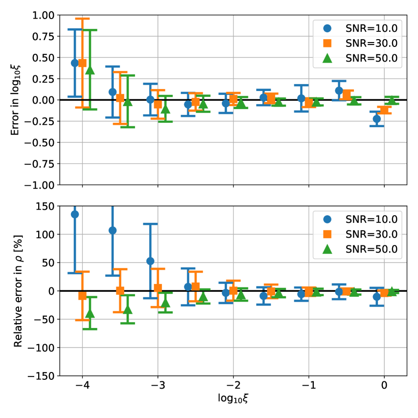
To further check the performance in detail, in the left panel of Fig. 6, we plot the average errors of (top) and (bottom) for different fiducial parameter values. The error bars indicate their standard deviations. To make this plot, we sample from to by the interval of . For each duty cycle, we prepare datasets with SNR , , and . Each dataset contains realizations. Note that we do not use the relative error for because the target value can be close to zero, which causes divergence in the relative error. First, we find from both left panels that the error variance reasonably increases as the SNR decreases. The estimation of the duty cycle and SNR seems not to be biased except when the fiducial value is at the border of the training range ( and ), and the SNR is small ().
In the right panels of Fig. 6, we show the results in which we include lower values of the duty cycle for the training, . We find that the error variances of both the duty cycle and the SNR significantly increase as the duty cycle decreases for . For the duty cycle, the systematic bias is smaller than the variance. On the other hand, for the SNR, we find a clear bias that the neural network tends to output a larger SNR than the true value when and a smaller SNR when . We find from test runs that such biases tend to increase when we use a shorter data length. From this, we can infer that the bias arises because the data length is too short. In fact, with the data length of used throughout this paper, the burst can be absent in the strain data for .
V.2 Second approach: Classification problem
As a second approach, we consider the classification problem. we divide the range of duty cycle values into four categories and assign the class index as the following
| (36) |
Again, we use the residual network with the structure shown in Table. 3 and Fig. 3, but the last fully connected layer and the softmax layer are modified to have four-dimensional outputs.
The training procedure is as follows. The weight update is repeated for times. The input data are normalized in the same way as the detection problem (see Eq. (29)). The duty cycle is sampled from the log uniform distribution on , and the SNR is sampled from the uniform distribution on . The batch size is 512, and the update algorithm is Adam with the learning rate of . For the loss function, we use the cross-entropy loss Eq. (25) with .

The trained neural network is tested with four datasets; each consists of 512 data and corresponds to the different classes. In the same way as the training data, SNRs are uniformly sampled from the range [1, 60] for all test datasets. Figure 7 presents the confusion matrix of the classification by the residual network. We find that 93.1% of test data are successfully classified to the correct class on average. Also, unlike the direct parameter estimation shown in the previous subsection, we can see that the residual neural network works well even for small values of the duty cycle . Thus, this method could be useful for giving an order of magnitude estimation of the duty cycle.


Now, we further investigate the misclassified cases. Figure 8 shows the scatter plot of misclassified events in the (, ) plane. It clearly shows that the duty cycles of the misclassified events are located at the boundary of the neighboring classes. As for the SNR distribution, we find that it is almost uniform, but as expected, there is a tendency that misclassification occurs more for . The colors of the dots in the scatter plot represent the maximum values of (the probability of each class), which indicates how confidently the neural network predicts the class. We can see that most of the misclassified events are given with low confidence.
Figure 9 shows the cumulative histograms (cumulating in the reverse direction of ) for correctly classified events and misclassified events. We can see a clear difference between them. For most of the correctly classified events, the probability of close to 1 is assigned. On the other hand, we can again see that misclassified events tend to have low confidence. However, of the events are misclassified with . As seen from Fig. 8, they are at the boundary of the neighboring classes, and this would be unavoidable with the classification problem method.
VI Conclusion
In this work, we studied applications of convolutional neural networks to the detection and parameter estimation of non-Gaussian stochastic GWs. As for the detection problem, we compared three different configurations of neural networks; shallower CNN, deeper CNN, and residual network. We found that the residual network can achieve comparable sensitivity to the maximum likelihood statistics. We also showed that neural networks have an advantage in computational time compared to the non-Gaussian statistic.
Next, we investigated the estimation of the duty cycle by a neural network with two different approaches. In the first approach, we trained the residual neural network to directly estimate the values of the duty cycle and SNR. We found that the estimation error in is about . As for SNR, the neural network can estimate with the relative error of . We found that the estimation of the duty cycle gets biased when we include a small duty cycle for the training . This could be explained by the shortness of the data length used in this paper. In the second approach, the parameter estimation was reduced to the classification problem in which the neural network classifies the data depending on the duty cycle. The parameter range was , and it was divided into four classes with the band of . The neural network could classify the data with an accuracy of 93% on average.
The present work is the first attempt to apply deep learning to the astrophysical GW background. In this work, we employed the toy model that is used in DF03 where various realistic effects, such as the detector’s configuration, noise properties, and waveform model of the bursts are neglected. In particular, detection of the astrophysical GW background would become challenging in the presence of glitch noises and the correlated magnetic noise from Schumann resonances. Further study of their effects will be extremely important for applying our method to real data. We leave it as future work with an expectation that deep learning has a high potential to distinguish such troublesome noises from the signal.
Acknowledgements.
This work is supported by JSPS KAKENHI Grant no. JP20H01899. TSY is supported by JSPS KAKENHI Grant no. JP17H06358 (and also JP17H06357), A01: Testing gravity theories using gravitational waves, as a part of the innovative research area, “Gravitational wave physics and astronomy: Genesis”. SK acknowledges support from the research project PGC2018-094773-B-C32, and the Spanish Research Agency through the Grant IFT Centro de Excelencia Severo Ochoa No CEX2020-001007-S, funded by MCIN/AEI/10.13039/501100011033. SK is supported by the Spanish Atracción de Talento contract no. 2019-T1/TIC-13177 granted by Comunidad de Madrid, the I+D grant PID2020-118159GA-C42 of the Spanish Ministry of Science and Innovation, the i-LINK 2021 grant LINKA20416 of CSIC, and JSPS KAKENHI Grant no. JP20H05853. This work was also supported in part by the Ministry of Science and Technology (MOST) of Taiwan, R.O.C., under Grants No. MOST 110-2123-M-007-002 and 110-2112-M-032 -007- (G.C.L.) The authors thank Joseph D. Romano for very useful comments.Appendix A Review of non-Gaussian statistic
Here, we review the properties of the non-Gaussian statistic (7). DF03 compared the non-Gaussian statistic with the standard cross-correlation statistic that is defined by
| (37) |
where
| (38) |
and is the Heaviside step function defined by
| (39) |
This is obtained by assuming the Gaussian signal model, i.e., in Eq. (5).
Here we aim to reproduce the results of DF03 and demonstrate the performance of Eq. (7) by simulating time series strain data with the length . The maximization of in Eq. (7) requires to explore the parameter space. Here, by following DF03, we substitute the injected values into instead of maximizing the model parameters. Note that we perform the parameter search to simulate the non-Gaussian statistic for the comparison purpose in the main part of the paper, but the general behavior does not change.
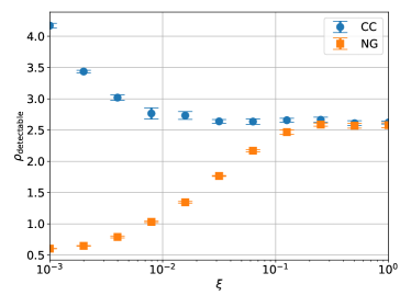
Figure 10 compares the minimum detectable SNR for the standard cross-correlation statistic and the non-Gaussian statistic. For , their performances are comparable. This can be interpreted that the non-Gaussianity of the signal is not much strong, and taking into account non-Gaussianity does not give a significant advantage. On the other hand, for , the non-Gaussian statistic outperforms the cross-correlation statistic. It is reasonable because the non-Gaussian statistic is developed based on the same signal model as the one we used for simulating strain data.

Next, parameter estimation is tested. Figure 11 shows an example of the distribution of the logarithm of in the plane. We injected a stochastic signal with and . It is clearly seen that the duty cycle and the amplitude variance of each burst degenerate. We also draw three dashed lines corresponding to different SNRs, 20, 40, and 60. We clearly see that the strong degeneracy exists along the line of constant SNR. In other words, the non-Gaussian statistic is sensitive to the difference in SNR.
References
- Abbott et al. [2016] B. P. Abbott et al. (LIGO Scientific, Virgo), Phys. Rev. Lett. 116, 131102 (2016), arXiv:1602.03847 [gr-qc] .
- Abbott et al. [2018] B. P. Abbott et al. (LIGO Scientific, Virgo), Phys. Rev. Lett. 120, 091101 (2018), arXiv:1710.05837 [gr-qc] .
- Abbott et al. [2021] R. Abbott et al. (KAGRA, Virgo, LIGO Scientific), Phys. Rev. D 104, 022004 (2021), arXiv:2101.12130 [gr-qc] .
- Braglia et al. [2022] M. Braglia, J. Garcia-Bellido, and S. Kuroyanagi, arXiv:2201.13414 [astro-ph.CO] (2022).
- Drasco and Flanagan [2003] S. Drasco and E. E. Flanagan, Phys. Rev. D 67, 082003 (2003), arXiv:gr-qc/0210032 .
- Thrane [2013] E. Thrane, Phys. Rev. D 87, 043009 (2013), arXiv:1301.0263 [astro-ph.IM] .
- Martellini and Regimbau [2014] L. Martellini and T. Regimbau, Phys. Rev. D 89, 124009 (2014), arXiv:1405.5775 [astro-ph.CO] .
- Martellini and Regimbau [2015] L. Martellini and T. Regimbau, Phys. Rev. D 92, 104025 (2015), [Erratum: Phys.Rev.D 97, 049903 (2018)], arXiv:1509.04802 [astro-ph.CO] .
- Cornish and Romano [2015] N. J. Cornish and J. D. Romano, Phys. Rev. D 92, 042001 (2015), arXiv:1505.08084 [gr-qc] .
- Seto [2008] N. Seto, Astrophys. J. Lett. 683, L95 (2008), arXiv:0807.1151 [astro-ph] .
- Seto [2009] N. Seto, Phys. Rev. D 80, 043003 (2009), arXiv:0908.0228 [gr-qc] .
- Smith and Thrane [2018] R. Smith and E. Thrane, Phys. Rev. X 8, 021019 (2018), arXiv:1712.00688 [gr-qc] .
- Smith et al. [2020] R. J. E. Smith, C. Talbot, F. Hernandez Vivanco, and E. Thrane, Mon. Not. Roy. Astron. Soc. 496, 3281 (2020), arXiv:2004.09700 [astro-ph.HE] .
- Biscoveanu et al. [2020] S. Biscoveanu, C. Talbot, E. Thrane, and R. Smith, Phys. Rev. Lett. 125, 241101 (2020), arXiv:2009.04418 [astro-ph.HE] .
- Matas and Romano [2021] A. Matas and J. D. Romano, Phys. Rev. D 103, 062003 (2021), arXiv:2012.00907 [gr-qc] .
- Romano and Cornish [2017] J. D. Romano and N. J. Cornish, Living Rev. Rel. 20, 2 (2017), arXiv:1608.06889 [gr-qc] .
- George and Huerta [2018a] D. George and E. A. Huerta, Phys. Rev. D 97, 044039 (2018a), arXiv:1701.00008 [astro-ph.IM] .
- George and Huerta [2018b] D. George and E. A. Huerta, Phys. Lett. B 778, 64 (2018b), arXiv:1711.03121 [gr-qc] .
- Gabbard et al. [2019] H. Gabbard, C. Messenger, I. S. Heng, F. Tonolini, and R. Murray-Smith, arXiv:1909.06296 [astro-ph.IM] (2019).
- Chua and Vallisneri [2020] A. J. K. Chua and M. Vallisneri, Phys. Rev. Lett. 124, 041102 (2020), arXiv:1909.05966 [gr-qc] .
- Green et al. [2020] S. R. Green, C. Simpson, and J. Gair, Phys. Rev. D 102, 104057 (2020), arXiv:2002.07656 [astro-ph.IM] .
- Dax et al. [2021] M. Dax, S. R. Green, J. Gair, J. H. Macke, A. Buonanno, and B. Schölkopf, Phys. Rev. Lett. 127, 241103 (2021), arXiv:2106.12594 [gr-qc] .
- Kuo and Lin [2022] H.-S. Kuo and F.-L. Lin, Phys. Rev. D 105, 044016 (2022), arXiv:2107.10730 [gr-qc] .
- Gabbard et al. [2018] H. Gabbard, M. Williams, F. Hayes, and C. Messenger, Phys. Rev. Lett. 120, 141103 (2018), arXiv:1712.06041 [astro-ph.IM] .
- Chatterjee et al. [2021] C. Chatterjee, L. Wen, F. Diakogiannis, and K. Vinsen, Phys. Rev. D 104, 064046 (2021), arXiv:2105.03073 [gr-qc] .
- Mishra et al. [2022] T. Mishra et al., Phys. Rev. D 105, 083018 (2022), arXiv:2201.01495 [gr-qc] .
- Nakano et al. [2019] H. Nakano, T. Narikawa, K.-i. Oohara, K. Sakai, H.-a. Shinkai, H. Takahashi, T. Tanaka, N. Uchikata, S. Yamamoto, and T. S. Yamamoto, Phys. Rev. D 99, 124032 (2019), arXiv:1811.06443 [gr-qc] .
- Shen et al. [2022] H. Shen, E. A. Huerta, E. O’Shea, P. Kumar, and Z. Zhao, Mach. Learn. Sci. Tech. 3, 015007 (2022), arXiv:1903.01998 [gr-qc] .
- Yamamoto and Tanaka [2020] T. S. Yamamoto and T. Tanaka, arXiv:2002.12095 [gr-qc] (2020).
- Bhagwat and Pacilio [2021] S. Bhagwat and C. Pacilio, Phys. Rev. D 104, 024030 (2021), arXiv:2101.07817 [gr-qc] .
- Morawski et al. [2020] F. Morawski, M. Bejger, and P. Cieciel\ag, Mach. Learn. Sci. Tech. 1, 025016 (2020), arXiv:1907.06917 [astro-ph.IM] .
- Dreissigacker et al. [2019] C. Dreissigacker, R. Sharma, C. Messenger, R. Zhao, and R. Prix, Phys. Rev. D 100, 044009 (2019), arXiv:1904.13291 [gr-qc] .
- Beheshtipour and Papa [2020] B. Beheshtipour and M. A. Papa, Phys. Rev. D 101, 064009 (2020), arXiv:2001.03116 [gr-qc] .
- Yamamoto and Tanaka [2021] T. S. Yamamoto and T. Tanaka, Phys. Rev. D 103, 084049 (2021), arXiv:2011.12522 [gr-qc] .
- Yamamoto et al. [2022] T. S. Yamamoto, A. L. Miller, M. Sieniawska, and T. Tanaka, Phys. Rev. D 106, 024025 (2022), arXiv:2206.00882 [gr-qc] .
- Astone et al. [2018] P. Astone, P. Cerdá-Durán, I. Di Palma, M. Drago, F. Muciaccia, C. Palomba, and F. Ricci, Phys. Rev. D 98, 122002 (2018), arXiv:1812.05363 [astro-ph.IM] .
- Morrás et al. [2022] G. Morrás, J. García-Bellido, and S. Nesseris, Phys. Dark Univ. 35, 100932 (2022), arXiv:2110.08000 [astro-ph.HE] .
- Utina et al. [2021] A. Utina, F. Marangio, F. Morawski, A. Iess, T. Regimbau, G. Fiameni, and E. Cuoco, in International Conference on Content-Based Multimedia Indexing (2021).
- Allen and Romano [1999] B. Allen and J. D. Romano, Phys. Rev. D 59, 102001 (1999), arXiv:gr-qc/9710117 .
- He et al. [2015] K. He, X. Zhang, S. Ren, and J. Sun, arXiv:1512.03385 [cs.CV] (2015).
- Ioffe and Szegedy [2015] S. Ioffe and C. Szegedy, arXiv:1502.03167 [cs.LG] (2015).
- Kingma and Ba [2014] D. P. Kingma and J. Ba, arXiv:1412.6980 [cs.LG] (2014).
- Paszke et al. [2019] A. Paszke, S. Gross, F. Massa, A. Lerer, J. Bradbury, G. Chanan, T. Killeen, Z. Lin, N. Gimelshein, L. Antiga, A. Desmaison, A. Köpf, E. Yang, Z. DeVito, M. Raison, A. Tejani, S. Chilamkurthy, B. Steiner, L. Fang, J. Bai, and S. Chintala, arXiv:1912.01703 [cs.LG] (2019).