Deep learning for full-field ultrasonic characterization
Abstract
This study takes advantage of recent advances in machine learning to establish a physics-based data analytic platform for distributed reconstruction of mechanical properties in layered components from full waveform data. In this vein, two logics, namely the direct inversion and physics-informed neural networks (PINNs), are explored. The direct inversion entails three steps: (i) spectral denoising and differentiation of the full-field data, (ii) building appropriate neural maps to approximate the profile of unknown physical and regularization parameters on their respective domains, and (iii) simultaneous training of the neural networks by minimizing the Tikhonov-regularized PDE loss using data from (i). PINNs furnish efficient surrogate models of complex systems with predictive capabilities via multitask learning where the field variables are modeled by neural maps endowed with (scaler or distributed) auxiliary parameters such as physical unknowns and loss function weights. PINNs are then trained by minimizing a measure of data misfit subject to the underlying physical laws as constraints. In this study, to facilitate learning from ultrasonic data, the PINNs loss adopts (a) wavenumber-dependent Sobolev norms to compute the data misfit, and (b) non-adaptive weights in a specific scaling framework to naturally balance the loss objectives by leveraging the form of PDEs germane to elastic-wave propagation. Both paradigms are examined via synthetic and laboratory test data. In the latter case, the reconstructions are performed at multiple frequencies and the results are verified by a set of complementary experiments highlighting the importance of verification and validation in data-driven modeling.
keywords:
deep learning, ultrasonic testing, data-driven mechanics, full-wavefield inversion1 Introduction
Recent advances in laser-based ultrasonic testing has led to the emergence of dense spatiotemporal datasets which along with suitable data analytic solutions may lead to better understanding of the mechanics of complex materials and components. This includes learning of distributed mechanical properties from test data which is of interest in a wide spectrum of applications from medical diagnosis to additive manufacturing [1, 2, 3, 4, 5, 6, 7]. This work makes use of recent progress in deep learning [8, 9] germane to direct and inverse problems in partial differential equations [10, 11, 12, 13] to develop a systematic full-field inversion framework to recover the profile of pertinent physical quantities in layered components from laser ultrasonic measurements. The focus is on two paradigms, namely: the direct inversion and physics-informed neural networks (PINNs) [14, 15, 16, 17]. The direct inversion approach is in fact the authors’ rendition of elastography method [18, 19, 20] through the prism of deep learning. To this end, tools of signal processing are deployed to (a) denoise the experimental data, and (b) carefully compute the required field derivatives as per the governing equations. In parallel, the unknown distribution of PDE parameters in space-frequency are identified by neural networks which are then trained by minimizing the single-objective elastography loss. The learning process is stabilized via the Tikhonov regularization [21, 22] where the regularization parameter is defined in a distributed sense as a separate neural network which is simultaneously trained with the sought-for physical quantities. This unique exercise of learning the regularization field without a-priori estimates, thanks to neural networks, proved to be convenient, effective, and remarkably insightful in inversion of multi-fidelity experimental data.
PINNs have recently come under the spotlight for offering efficient, yet predictive, models of complex PDE systems [10] that has so far been backed by rigorous theoretical justification within the context of linear elliptic and parabolic PDEs [23]. Given the multitask nature of training for these networks and the existing challenges with modeling stiff and highly oscillatory PDEs [12, 24], much of the most recent efforts has been focused on (a) adaptive gauging of the loss function [12, 25, 26, 27, 28, 29, 13], and (b) addressing the gradient pathologies [24, 13] e.g., via learning rate annealing [30] and customizing the network architecture [11, 31, 32]. In this study, our initially austere implementations of PINNs using both synthetic and experimental waveforms led almost invariably to failure which further investigation attributed to the following impediments: (a) high-norm gradient fields due to large wavenumbers, (b) high-order governing PDEs in the case of laboratory experiments, and (c) imbalanced objectives in the loss function. These problems were further magnified by our attempts for distributed reconstruction of discontinuous PDE parameters – in the case of laboratory experiments, from contaminated and non-smooth measurements. The following measures proved to be effective in addressing some of these challenges: (i) training PINNs in a specific scaling framework where the dominant wavenumber is the reference length scale, (ii) using the wavenumber-dependent Sobolev norms in quantifying the data misfit, (iii) taking advantage of the inertia term in the governing PDEs to naturally balance the objectives in the loss function, and (iv) denoising of the experimental data prior to training.
This paper is organized as follows. Section 2 formulates the direct scattering problem related to the synthetic and laboratory experiments, and provides an overview of the data inversion logic. Section 3 presents the computational implementation of direct inversion and PINNs to reconstruct the distribution of Láme parameters in homogeneous and heterogeneous models from in-plane displacement fields. Section 4 provides a detailed account of laboratory experiments, scaling, signal processing, and inversion of antiplane particle velocity fields to recover the distribution of a physical parameter affiliated with flexural waves in thin plates. The reconstruction results are then verified by a set of complementary experiments.
2 Concept
This section provides (i) a generic formalism for the direct scattering problem pertinent to the ensuing (synthetic and experimental) full-field characterizations, and (ii) data inversion logic.
2.1 Forward scattering problem
Consider ultrasonic tests where the specimen , , is subject to (boundary or internal) excitation over the incident surface and the induced (particle displacement or velocity) field () is captured over the observation surface in a timeframe of length . Here, is an open set whose closure is denoted by , and the sensing configuration is such that . In this setting, the spectrum of observed waveforms is governed by
| (1) |
where of size designates a differential operator in frequency-space; represents the temporal Fourier transform; of dimension is the vector of relevant geometric and elastic parameters e.g., Lamé constants and mass density; is the position vector; and is the frequency of wave motion within the specified bandwidth .
2.2 Dimensional platform
2.3 Data inversion
Given the full waveform data on , the goal is to identify the distribution of material properties over . For this purpose, two reconstruction paradigms based on neural networks are adopted in this study, namely: (i) direct inversion, and (ii) physics-based neural networks. Inspired by the elastography method [18, 19], quantities of interest in (i) are identified by neural maps over that minimize a regularized measure of in (1). The neural networks in (ii), however, are by design predictive maps of the waveform data (i.e., ) obtained by minimizing the data mismatch subject to (1) as a soft or hard constraint. In this setting, the unknown properties of may be recovered as distributed parameters of the (data) network during training via multitask optimization. In what follows, a detailed description of the deployed cost functions in (i) and (ii) is provided after a brief review of the affiliated networks.
2.3.1 Waveform and parameter networks
Laser-based ultrasonic experiments furnish a dense dataset on . Based on this, multilayer perceptrons (MLPs) owing to their dense range [34] may be appropriate for approximating complex wavefields and distributed PDE parameters. Moreover, this architecture has proven successful in numerous applications within the PINN framework [15]. In this study, MLPs serve as both data and property maps where the input consists of discretized space and frequency coordinates , , , as well as distinct experimental parameters, e.g., the source location, distilled as one vector on domain with , while the output represents waveform data , and/or the sought-for mechanical properties , . Note that following [35], the real and imaginary parts of (1) and every complex-valued variable are separated such that both direct and inverse problems are reformulated in terms of real-valued quantities. In this setting, each fully-connected MLP layer with neurons is associated with the forward map ,
| (2) |
where and respectively denote the layer’s weight and bias. Consecutive composition of for builds the network map wherein designates the number of layers.
2.3.2 Direct inversion
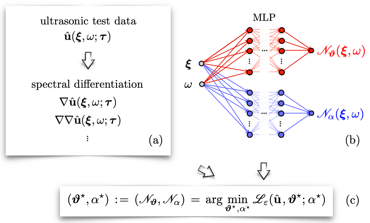
Logically driven by the elastography method, the direct inversion approach depicted in Fig. 1 takes advantage of the leading-order physical principles underpinning the test data to recover the distribution of relevant physical quantities in space-frequency i.e., over the measurement domain. The ML-based direct inversion entails three steps: (a) spectral denoising and differentiation of (n-differentiable) waveforms over according to the (n-th order) governing PDEs in (1), (b) building appropriate MLP maps to estimate the profile of unknown physical parameters of the forward problem and regularization parameters of the inverse solution, and (c) learning the MLPs through regularized fitting of data to the germane PDEs.
Note that synthetic datasets – generated via e.g., computer modeling or the method of manufactured solutions, may directly lend themselves to the fitting process in (c) as they are typically smooth by virtue of numerical integration or analytical form of the postulated solution. Laboratory test data, however, are generally contaminated by noise and uncertainties, and thus, spectral differentiation is critical to achieve the smoothness requirements in (c). The four-tier signal processing of experimental data follows closely that of [36, Section 3.1] which for completeness is summarized here: (1) a band-pass filter consistent with the frequency spectrum of excitation is applied to the measured time signals at every receiver point, (2) the obtained temporally smooth signals are then differentiated or integrated to obtain the pertinent field variables, (3) spatial smoothing is implemented at every snapshot in time via application of median and moving average filters followed by computing the Fourier representation of the processed waveforms in space, (4) the resulting smooth fields may be differentiated (analytically in the Fourier space) as many times as needed based on the underlying physical laws in preparation for the full-field reconstruction in step (c). It should be mentioned that the experimental data may feature intrinsic discontinuities e.g., due to material heterogeneities or contact interfaces. In this case, the spatial smoothing in (3) must be implemented in a piecewise manner after the geometric reconstruction of discontinuity surfaces in which is quite straightforward thanks to the full-field measurements, see e.g., [36, section 3.2].
Next, the unknown PDE parameters are approximated by a fully connected MLP network as per Section 2.3.1. The network is trained by minimizing the loss function
| (3) |
where indicates an all-ones vector of dimension , and designates the (element-wise) Hadamard product. Here, the PDE residual based on (1) is penalized by the norm of unknown parameters. Observe that the latter is a function of the weights and biases of the neural network which may help stabilize the MLP estimates during optimization. Such Tikhonov-type functionals are quite common in waveform tomography applications [37, 38, 39] owing to their well-established regularizing properties [21, 22]. Within this framework, is the regularization parameter which may be determined by three means, namely: (i) the Morozov discrepancy principle [40, 41], (ii) its formulation as a (constant or distributed) parameter of the network which could then be learned during training, and (iii) its independent reconstruction as a separate MLP network illustrated in Fig. 1 (b) that is simultaneously trained along with by minimizing (3). In this study, direct inversion is applied to synthetic and laboratory test data with both and , based on (ii) and (iii). It was consistently observed that the regularization parameter plays a key role in controlling the MLP estimates. This is particularly the case in situations where the field is strongly polarized or near-zero in certain neighborhoods which brings about instability i.e., very large estimates for in these areas. In light of this, all direct inversion results in this paper correspond to the case of identified by the MLP network .
2.3.3 Physics-informed neural networks
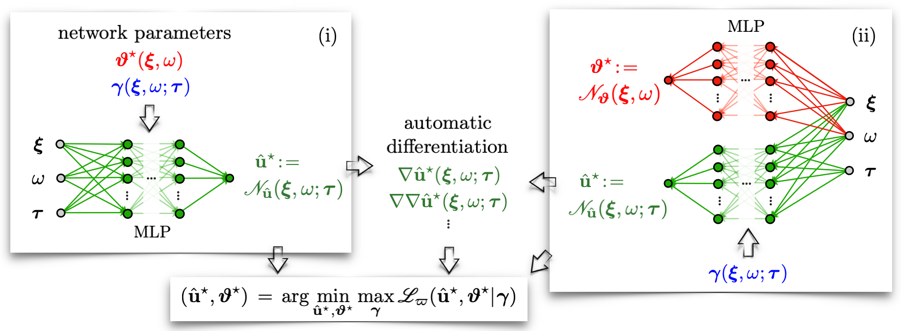
By deploying the knowledge of underlying physics, PINNs [14, 15] furnish efficient neural models of complex PDE systems with predictive capabilities. In this vein, a multitask learning process is devised according to Fig. 2 where (a) the field variable – i.e., measured data on , is modeled by the MLP map endowed with the auxiliary parameter related to the loss function (4), (b) the physical unknowns could be defined either as parameters of as in Fig. 2 (i), or as a separate MLP as shown in Fig. 2 (ii), and (c) learning the MLPs and affiliated parameters through minimizing a measure of data misfit subject to the governing PDEs as soft/hard constraints wherein the spatial derivatives of are computed via automatic differentiation [42]. It should be mentioned that in this study all MLP networks are defined on (a subset of) where . Hence, the initial and boundary conditions – which could be specified as additional constraints in the loss function [15], are ignored. In this setting, the PINNs loss takes the form
| (4) |
where is a vector of ones; n is the order of , and denotes the adaptive norm defined by
| (5) |
Here, is a vector of integers . Provided that , then is by definition equal to [43]. Note however that at high wavenumbers, is dominated by the highest derivatives , , which may complicate (or even lead to the failure of) the training process due to uncontrolled error amplification by automatic differentiation particularly in earlier epochs. This issue may be addressed through proper weighting of derivatives in (5). In light of the frequency-dependent Sobolev norms in [44, 37], one potential strategy is to adopt the wavenumber-dependent weights as the following
wherein is a measure of wavenumber along for . In this setting, the weighted norms of derivatives in (5) remain approximately within the same order as the norm of data misfit. Another way to automatically achieve the latter is to set the reference scale such that . Note that the norms directly inform the PINNs about the “expected” field derivatives – while preventing their uncontrolled magnification. This may help stabilize the learning process as such derivatives are intrinsically involved in the PINNs loss via . It should be mentioned that when in (4), the “true” estimates for derivatives may be obtained via spectral differentiation as per Section 2.3.2.
The Lagrange multiplier [45, 46] in (4) is critical for balancing the loss components during training. Its optimal value, however, highly depends on (a) the nature of [12], and (b) the distribution of unknown parameters . It should be mentioned that setting led to failure in almost all of the synthetic and experimental implementations of PINNs in this study. Gauging of loss function weights has been the subject of extensive recent studies [12, 25, 47, 26, 27, 28]. One systematic approach is the adaptive SA-PINNs [12] where the multiplier is a distributed parameter of whose value is updated in each epoch according to a minimax weighting paradigm. Within this framework, the data (and parameter) networks are trained by minimizing with respect to and , while maximizing the loss with respect to as shown in Fig. 2.
Depending on the primary objective for PINNs, one may choose nonadaptive or adaptive weighting. More specifically, if the purpose is high-fidelity forward modeling via neural networks where is known a-priori and PINNs are intended to serve as predictive surrogate models of , then ideas rooted in constrained optimization e.g., minimax weighting is theoretically sound. However, if the inverse solution i.e., identification of from “real-world” or laboratory test data is the main goal particularly in a situation where any assumption on the smoothness of and/or applicability of may be (at least locally) violated e.g., due to unknown material heterogeneities or interfacial discontinuities, then trying to enforce everywhere on (via point-wise adaptive weighting) may lead to instability and failure of data inversion. In such cases, nonadaptive weighting may be more appropriate. In light of this, in what follows, is a non-adaptive weight specified by taking advantage of the PDE structure to naturally balance the loss objectives.
3 Synthetic implementation
Full-field characterization via the direct inversion and physics-informed neural networks are examined through a set of numerical experiments. The waveform data in this section are generated via a FreeFem++ [48] code developed as part of [49].
3.1 Problem statement
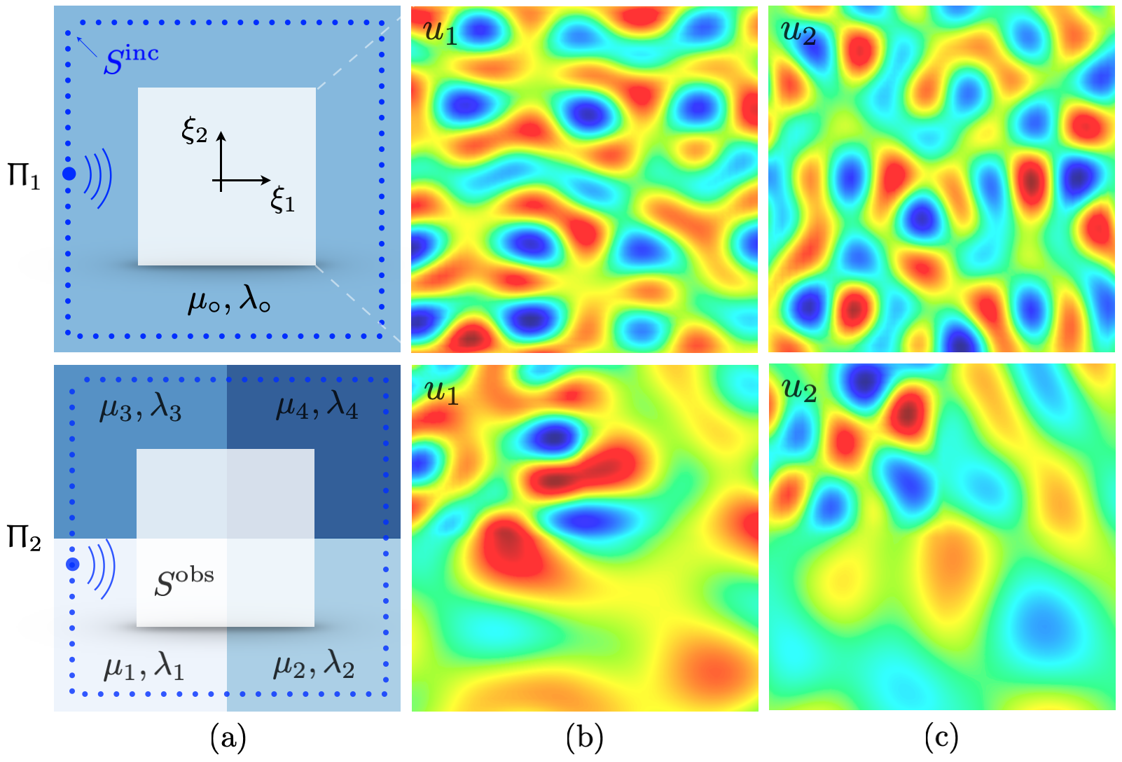
Plane-strain wave motion in two linear, elastic, piecewise homogeneous, and isotropic samples is modeled according to Fig. 3 (a). On denoting the frequency of excitation by , let , , and be the reference scales for length, mass density, and stress, respectively. In this framework, both specimens are of size and uniform density . The first sample is characterized by the constant Lamé parameters and , while the second sample is comprised of four perfectly bonded homogenous components of and , such that . Accordingly, the shear and compressional wave speeds read , in , and , in . Every numerical experiment entails an in-plane harmonic excitation at via a point source on (the perimeter of a square centered at the origin). The resulting displacement field , , is then computed in over (a concentric square of dimension ) such that
| (6) | |||||
where and respectively indicate the source location and polarization vector; is the unit outward normal to the specimen’s exterior, and
When , the first of (6) should be understood as a shorthand for the set of four governing equations over , , supplemented by the continuity conditions for displacement and traction across as applicable.
In this setting, the generic form (1) may be identified as the following
| (7) | |||||
wherein is the second-order identity tensor; with denoting the unit circle of polarization directions. Note that is treated here as a known parameter.
In the numerical experiments, (resp. ) is discretized by a uniform grid of 32 (resp. 50 50) points, while and are respectively sampled at and .
All inversions in this study are implemented within the PyTorch framework [50].
3.2 Direct inversion
The three-tier logic of Section 2.3.2 is employed to reconstruct the distribution of and , , over , entailing: (a) spectral differentiation of the displacement field in order to compute and as per (6), (b) construction of three positive-definite MLP networks , , and ; each of which is comprised of one hidden layer of 64 neurons, and (c) training the MLPs by minimizing as in (3) and (7) by way of the ADAM algorithm [51]. To avoid near-boundary errors affiliated with the one-sided FFT differentiation in and , a concentric subset of collocation points sampling is deployed for training purposes. It should also be mentioned that in the heterogeneous case, i.e., , the discontinuity of derivatives across calls for piecewise spectral differentiation. According to Section 2.3.1, the input to , , and is of size where is the number of simulations i.e., source locations used to generate distinct waveforms for training. In this setting, since the physical quantities of interest are independent of , the real-valued output of MLPs is of dimension furnishing a local estimate of the Láme and regularization parameters at the specified sampling points on . Each epoch makes use of the full dataset and the learning rate is .
In this work, the reconstruction error is measured in terms of the normal misfit
| (8) |
where is an MLP estimate for a quantity with the “true” value q.
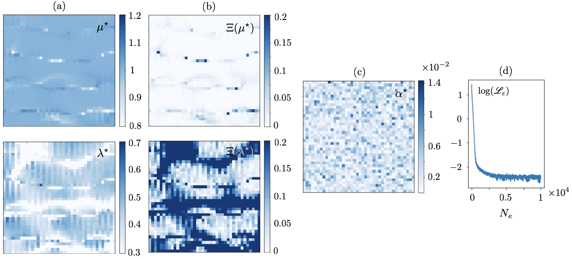
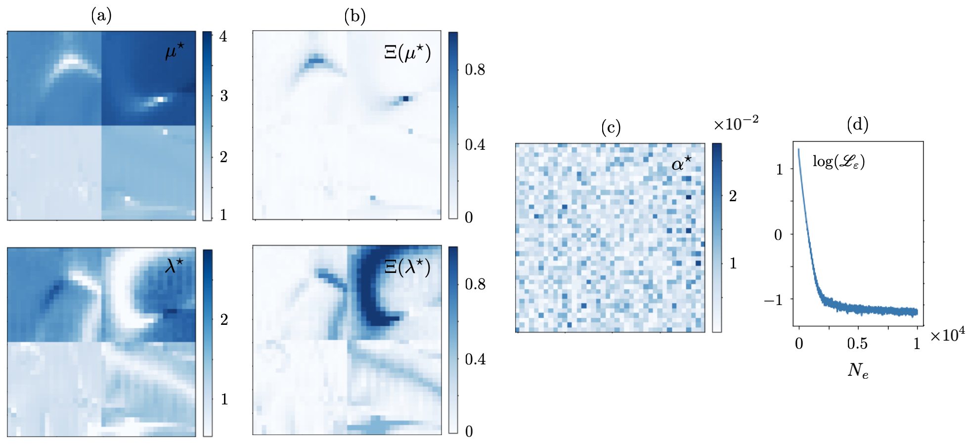
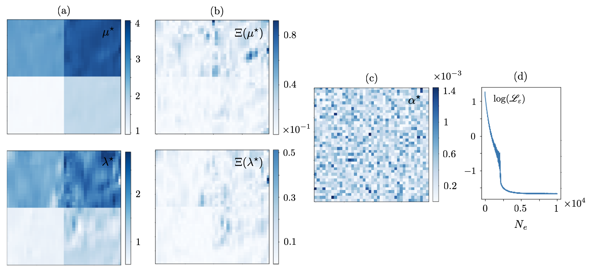
Let be sampled at one point i.e., so that a single forward simulation in , , generates the training dataset. The resulting reconstructions are shown in Figs. 4 and 5. It is evident from both figures that the single-source reconstruction fails at the loci of near-zero displacement which may explain the relatively high values of the recovered regularization parameter . Table 1 details the true values as well as mean and standard deviation of the reconstructed Láme distributions in (resp. for ) according to Fig. 4 (resp. Fig. 5).
This problem may be addressed by enriching the training dataset e.g., via increasing . Figs. 6 and 7 illustrate the reconstruction results when is sampled at source points. The mean and standard deviation of the reconstructed distributions are provided in Table 2. It is worth noting that in this case the identified regularization parameter assumes much smaller values – compared to that of Figs. 4 and 5. This is closer to the scale of computational errors in the forward simulations.
To examine the impact of noise on the reconstruction, the multisource dataset used to generate Figs. 6 and 7 are perturbed with white noise. The subsequent direct inversions from noisy data are displayed in Figs. 8 and 9, and the associated statistics are presented in Table 3. Note that spectral differentiation as the first step in direct inversion plays a critical role in denoising the waveforms, and subsequently regularizing the reconstruction process. This may substantiate the low magnitude of MLP-recovered in the case of noisy data in Figs. 8 and 9. The presence of noise, nonetheless, affects the magnitude and thus composition of terms in the Fourier representation of the processed displacement fields in space which is used for differentiation. This may in turn lead to the emergence of fluctuations in the reconstructed fields.
| | | | | | |
|---|---|---|---|---|---|
| | | | | | |
| | | | | | |
| | | | | | |
| | | | | |
| | | | | | |
|---|---|---|---|---|---|
| | | | | | |
| | | | | | |
| | | | | | |
| | | | | |
3.3 Physics-informed neural networks
The learning process of Section 2.3.3 is performed as follows: (a) the MLP network endowed with the positive-definite parameters and is constructed such that the input labels the source location and the auxiliary weight is a nonadaptive scaler, (b) and may be specified as scaler or distributed parameters of the network according to Fig. 2 (i), and (c) is trained by minimizing in (4) via the ADAM optimizer using the synthetic waveforms of Section 3.1. Reconstructions are performed on the same set of collocation points sampling as in Section 3.2. Accordingly, the input to is of size , while its output is of dimension modeling the displacement field along and in the sampling region. Similar to Section 3.2, each epoch makes use of the full dataset for training and the learning rate is . The PyTorch implementation of PINNs in this section is accomplished by building upon the available codes on the Github repository [52].
The MLP network with three hidden layers of respectively , , and neurons is employed to map the displacement field (in ) associated with a single point source of frequency at . The Láme constants are defined as the unknown scaler parameters of the network i.e., , and the Lagrange multiplier is specified per the following argument. Within the dimensional framework of this section and with reference to (7), observe that on setting (i.e., ), both (the PDE residue and data misfit) components of the loss function in 4 emerge as some form of balance in terms of the displacement field. This may naturally facilitate maintaining of the same scale for the loss terms during training, and thus, simplifying the learning process by dispensing with the need to tune an additional parameter . Keep in mind that the input to is of size , while its output is of dimension . In this setting, the training objective is two-fold: (a) construction of a surrogate map for , and (b) identification of and .
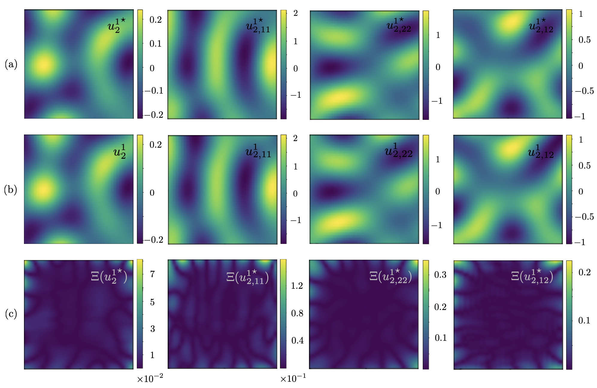
Fig. 10 showcases (i) the accuracy of PINN estimates based on noiseless data in terms of the vertical component of displacement field in , and (ii) the performance of automatic differentiation [42] in capturing the field derivatives in terms of components that appear in the governing PDE 7 i.e., , . The comparative analysis in (ii) is against the spectral derivates of FEM fields according to Section 2.3.2. It is worth noting that similar to Fourier-based differentiation, the most pronounced errors in automatic differentiation occur in the near-boundary region i.e., the support of one-sided derivatives. It is observed that the magnitude of such discrepancies may be reduced remarkably by increasing the number of epochs. Nonetheless, the loci of notable errors remain at the vicinity of specimen’s external boundary or internal discontinuities such as cracks or material interfaces. Fig. 10 is complemented with the reconstruction
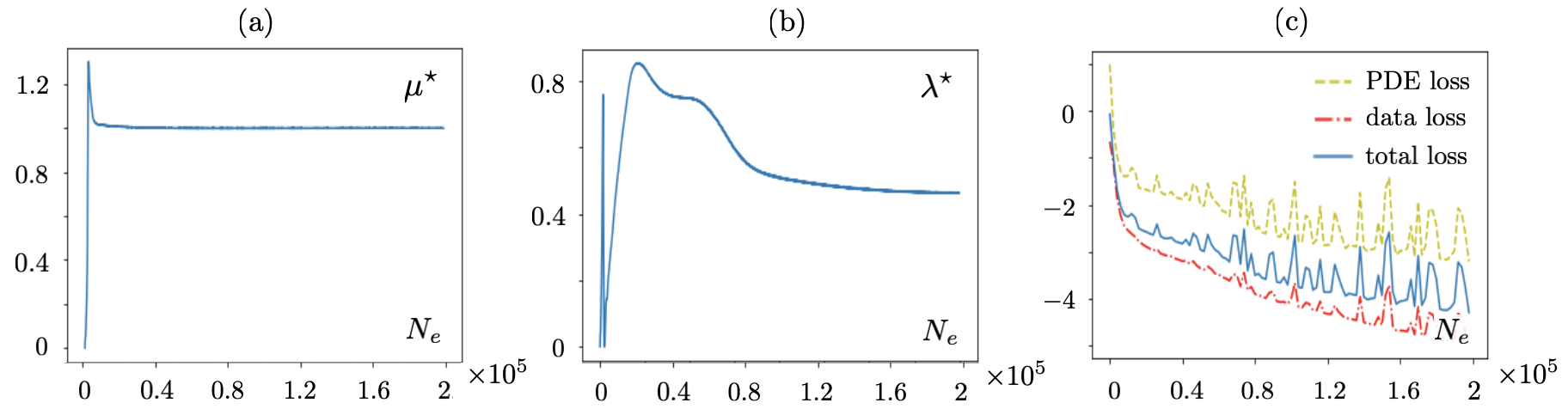
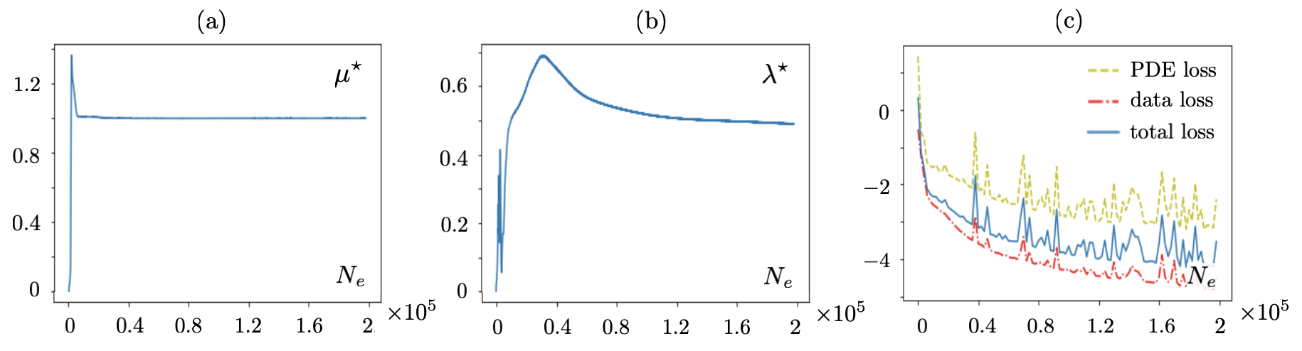
results of Fig. 11 indicating for the homogenous specimen with the true Láme constants . The impact of noise on training is examined by perturbing the noiseless data related to Fig. 10 with white noise, which led to as shown in Fig. 12.
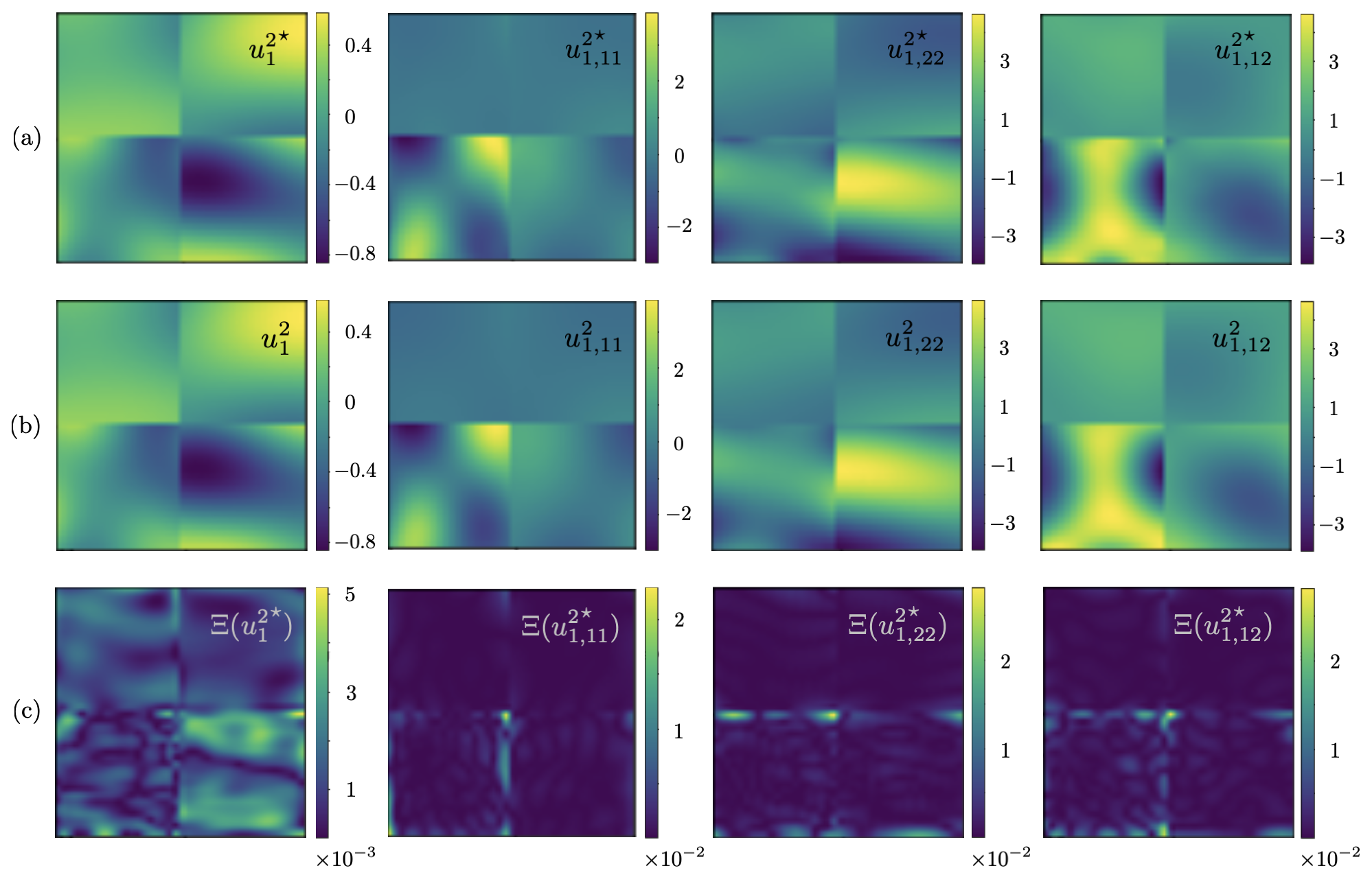
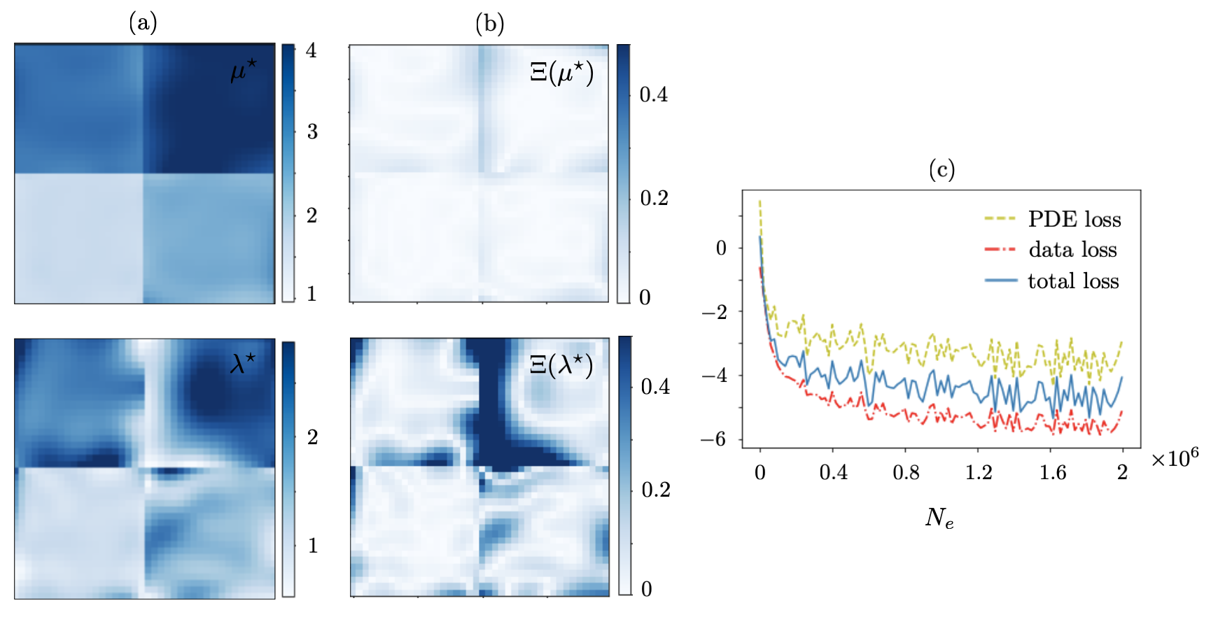
Next, the PINN with three hidden layers of respectively , , and neurons is created to reconstruct (i) displacement field in the heterogeneous specimen , and (ii) distribution of the Láme parameters over the observation surface. In this vein, synthetic waveform data associated with five point sources , at is used for training. Here, is the network’s unknown distributed parameter, of dimension , and the nonadaptive scaler weight in light of the sample’s uniform density . In this setting, the input to is of size , while its output is of dimension . Fig. 13 provides a comparative analysis between the FEM and PINN maps of horizontal displacement in and its spatial derivatives computed by spectral and automatic differentiation respectively.
| | | | | |
|---|---|---|---|---|
| . | ||||
| | | | | |
| | | | | |
| | | | |
4 Laboratory implementation
This section examines the performance of direct inversion and PINNs for full-field ultrasonic characterization in a laboratory setting. In what follows, experimental data are processed prior to inversion as per Section 2.3.2 which summarizes the detailed procedure in [36]. To verify the inversion results, quantities of interest are also reconstructed through dispersion analysis, separately, from a set of auxiliary experiments.
4.1 Test set-up
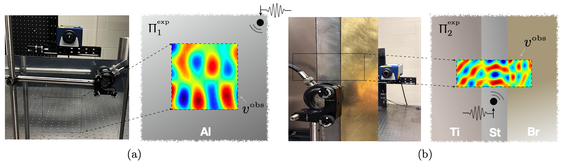
Experiments are performed on two (homogeneous and heterogeneous) specimens: which is a cm cm mm sheet of T6 6061 aluminum, and composed of (a) cm cm mm sheet of Grade 2 titanium, (b) cm cm mm sheet of 4130 steel, and (c) cm cm mm sheet of 260-H02 brass, connected via metal epoxy. For future reference, the density , Young’s modulus , and Poisson’s ratio for are listed in Table 5 as per the manufacturer.
Ultrasonic experiments on both samples are performed in a similar setting in terms of the sensing configuration and illuminating wavelet. In both cases, the specimen is excited by an antiplane shear wave from a designated source location , shown in Fig. 15, by a MHz p-wave piezoceramic transducer (V101RB by Olympus Inc.). The incident signal is a five-cycle burst of the form
| (9) |
where denotes the Heaviside step function, and the center frequency is set at kHz (resp. kHz) in (resp. ). The induced wave motion is measured in terms of the particle velocity , , on the scan grids sampling where . A laser Doppler vibrometer (LDV) which is mounted on a 2D robotic translation frame (for scanning) is deployed for measurements. The VibroFlex Xtra VFX-I-120 LDV system by Polytec Inc. is capable of capturing particle velocity within the frequency range MHz along the laser beam which in this study is normal to the specimen’s surface.
The scanning grid is identified by a cm cm square sampled by uniformly spaced measurement points. This amounts to a spatial resolution of mm in both spatial directions. In parallel, is a cm cm rectangle positioned according to Fig. 15 (b) and sampled by a uniform grid of scan points associated with the spatial resolution of mm. At every scan point, the data acquisition is conducted for a time period of s at the sampling rate of MHz. To minimize the impact of optical and mechanical noise in the system, the measurements are averaged over an ensemble of 80 realizations at each scan point. Bear in mind that both the direct inversion and PINNs deploy the spectra of normalized velocity fields for data inversion. Such distributions of out-of-plane particle velocity at kHz (resp. kHz) in (resp. ) is displayed in Fig. 15.
It should be mentioned that in the above experiments, the magnitude of measured signals in terms of displacement is of so that it may be appropriate to assume a linear regime of propagation. The nature of antiplane wave motion is dispersive nonetheless. Therefore, to determine the relevant length scales in each component, the associated dispersion curves are obtained as in Fig. 19 via a set of complementary experiments described in Section 4.4.1. Accordingly, for excitations of center frequency kHz, the affiliated phase velocity and wavelength for is identified in Table 6.
4.2 Dimensional framework
On recalling Section 2.2, let m, GPA, and kg/m3 be the reference scales for length, stress, and mass density, respectively. In this setting, the following maps take the physical quantities to their dimensionless values
| (10) | |||||
where mm and respectively indicate the specimen’s thickness and cyclic frequency of wave motion. Table 5 (resp. Table 6) details the normal values for the first (resp. second) of (10). The normal thickness and center frequencies are as follows,
| (11) |
| physical | | Al | Ti | St | Br |
|---|---|---|---|---|---|
| [GPA] | 68.9 | 105 | 199.95 | 110 | |
| quantity | [kg/m3] | 2700 | 4510 | 7850 | 8530 |
| | 0.33 | 0.34 | 0.29 | 0.31 | |
| normal | | 1 | 1.52 | 2.90 | 1.60 |
| value | | 1 | 1.67 | 2.91 | 3.16 |
| | 1 | 0.91 | 1 | 0.51 |
physical quantity Al Ti St Br [cm] [m/s] [cm] [m/s] [cm] [m/s]
normal value Al Ti St Br
4.3 Governing equation
In light of (11) and Table 6, observe that in all tests the wavelength-to-thickness ratio , . Therefore, one may invoke the equation governing flexural waves in thin plates [53] to approximate the physics of measured data. In this framework, (1) may be recast as
| (12) | |||||
where respectively denote the normal density, Young’s modulus, and Poisson’s ratio in , , and indicates the source location. Note that according to Table 5 and , related to , shows little sensitivity to small variations in the Poisson’s ratio. Thus, in what follows, is treated as a known parameter. Provided , the objective is to reconstruct .
4.4 Direct inversion
Following the reconstruction procedure of Section 3.2, the distribution of in , , is obtained at specific frequencies. In this vein, the positive-definite MLP networks and comprised of three hidden layers of respectively , , and neurons are constructed according to Fig. 1. In all MLP trainings of this section, each epoch makes use of the full dataset and the learning rate is .
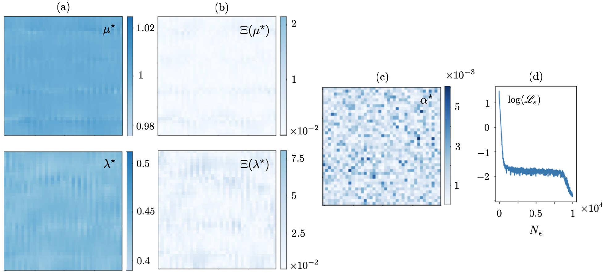
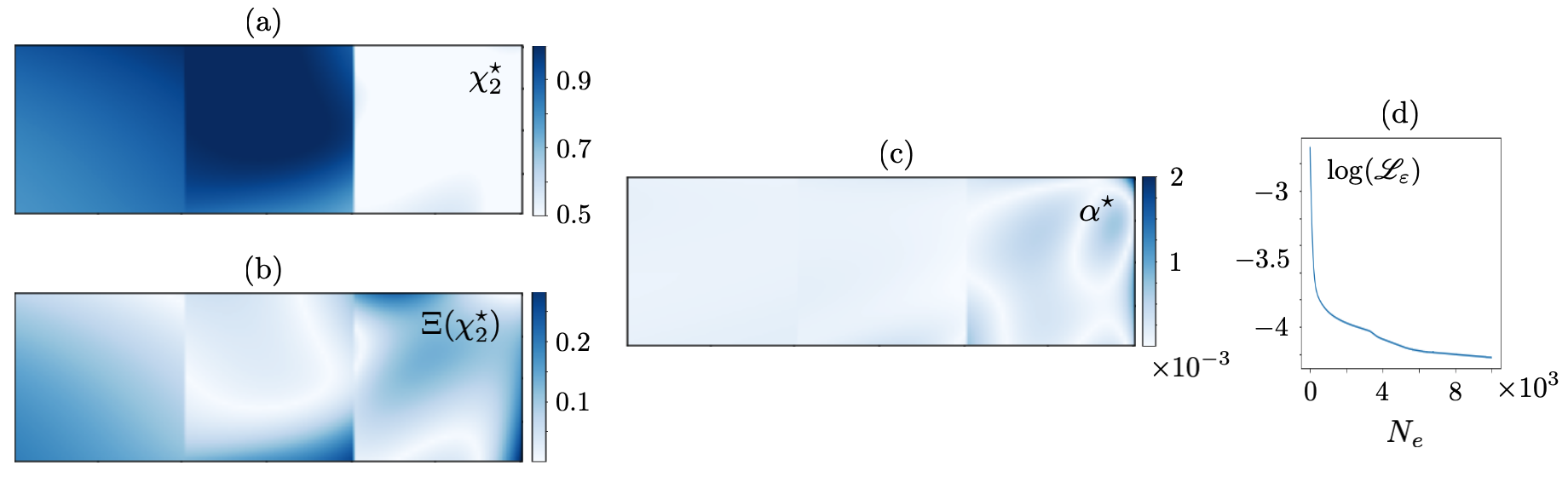
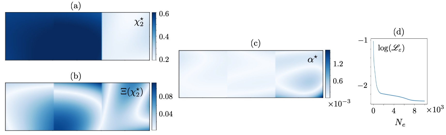
When , the inversion is conducted at . is sampled at one point i.e., the piezoelectric transducer remains fixed during the test on Al plate, and thus, , while a concentric subset of collocation points sampling is deployed for training. In this setting, the input to and is of size , and their real-valued outputs are of the same size. The results are shown in Fig. 16. When , the direct inversion is conducted at and . For the low-frequency reconstruction, is sampled at one point, while a subset of scan points in is used for training so that the input/output size for and is . The recovered fields and associated normal error are provided in Fig. 17. Table 7 enlists the true values as well as mean and standard deviation of the reconstructed distributions in , , according to Figs. 16 and 17. For the high-frequency reconstruction, when , is sampled at three points i.e., experiments are performed for three distinct positions of the piezoelectric transducer, while the same subset of scan points is used for training. In this case, the input to and is , while their output is of dimension . The high-frequency reconstruction results are illustrated in Fig. 18, and the affiliated means and standard deviations are provided in Table 8. It should be mentioned that the computed normal errors in Figs. 16, 17, and 18 are with respect to the verified values of Section 4.4.1. Note that the recovered s from laboratory test data are much smoother than the ones reconstructed from synthetic data in Section 3.2. This could be attributed to the scaler nature of (12) with a single unknown parameter – as opposed to the vector equations governing the in-plane wave motion with two unknown parameters. More specifically, here, controls the weights and biases of a single network , while in Section 3.2, simultaneously controls the parameters of two separate networks and . A comparative analysis of Figs. 17 and 18 reveals that (a) enriching the waveform data by increasing the number of sources remarkably decrease the reconstruction error, (b) the regularization parameter in (3) is truly distributed in nature as the magnitude of the recovered in brass is ten times greater than that of titanium and steel which is due to the difference in the level of noise in measurements related to distinct material surfaces, and (c) the recovered field – which according to (12) is a material property , demonstrates a significant dependence to the reconstruction frequency. The latter calls for proper verification of the results which is the subject of Section 4.4.1.
4.4.1 Verification
To shine some light on the nature discrepancies between the low- and high- frequency reconstructions in
| | | | | |
|---|---|---|---|---|
| | | | |
| | | | |
|---|---|---|---|
| | | | |
| | | |
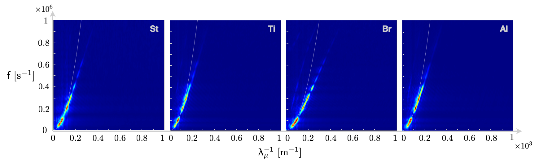
Figs. 17 and 18, a set of secondary tests are performed to obtain the dispersion curve for each component of the test setup. For this purpose, antiplane shear waves of form (9) are induced at kHz, , in cm cm cuts of aluminum, titanium, steel, and brass sheets used in the primary tests of Fig. 15. In each experiment, the piezoelectric transducer is placed in the middle of specimen (far from the external boundary), and the out-of-plane wave motion is captured in the immediate vicinity of the transducer along a straight line of length cm sampled at scan points. The Fourier-transformed signals in time-space furnish the dispersion relations of Fig. 19. In parallel, the theoretical dispersion curves affiliated with (12) are computed according to
| (13) |
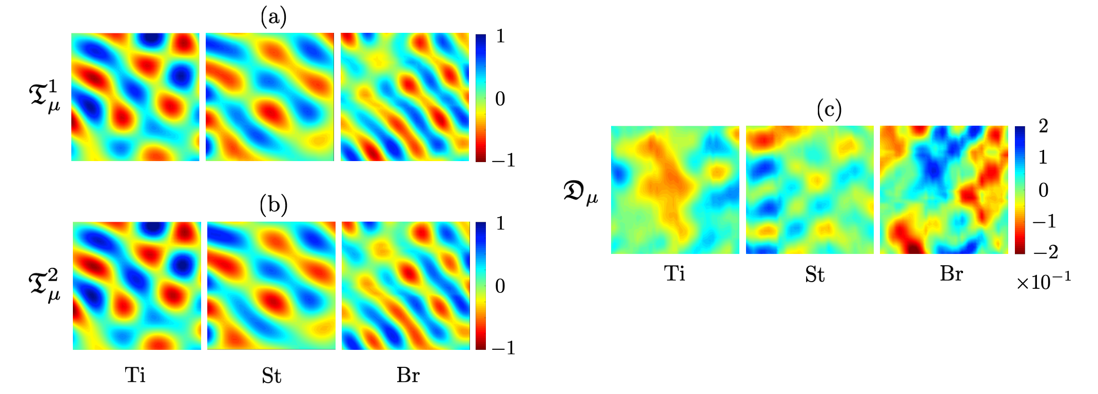
using the values of Table 5 for and and mm. A comparison between the experimental and theoretical dispersion curves in Fig. 19 verifies the theory and the values of Table 5 for in the low-frequency regime of wave motion. This is also in agreement with the direct inversion results of Figs. 16 and 17. Moreover, Fig. 19 suggests that at approximately kHz for the governing PDE (12) with physical coefficients fails to predict the experimental results which may provide an insight regarding the high-frequency reconstruction results in Fig. 18. Further investigation of the balance law (12), as illustrated in Fig. 20, shows that the test data at kHz satisfy – with less than discrepancy depending on the material – a PDE of form (12) with modified coefficients. More specifically, Fig. 20 demonstrates the achievable balance between the elastic force distribution and inertia field in (12) by directly adjusting the PDE parameter to minimize the discrepancy according to
| (14) |
With reference to Table 8, the recovered coefficients at verify the direct inversion results of Fig. 18. This implies that the direct inversion (or PINNs) may lead to non-physical reconstructions in order to attain the best fit for the data to the “perceived”” underlying physics. Thus, it is imperative to establish the range of validity of the prescribed physical principles in data-driven modeling. Here, the physics of the system at is in transition, yet close enough to the leading-order approximation (12) that the discrepancy is less than . It is unclear, however, if this equation with non-physical coefficients may be used as a predictive tool. It would be interesting to further investigate the results through the prism of higher-order continuum theories and a set of independent experiments for validation which could be the subject of a future study.
4.5 Physics-informed neural networks
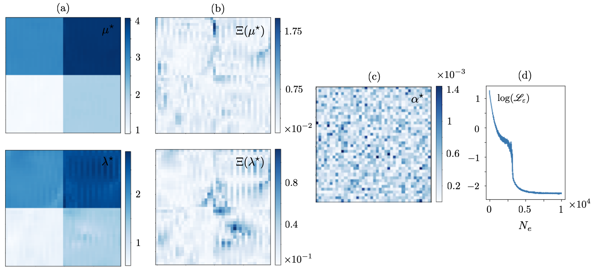
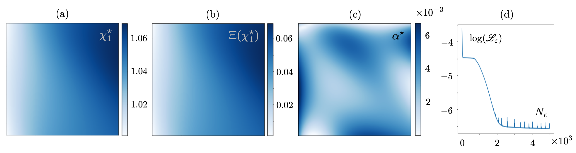
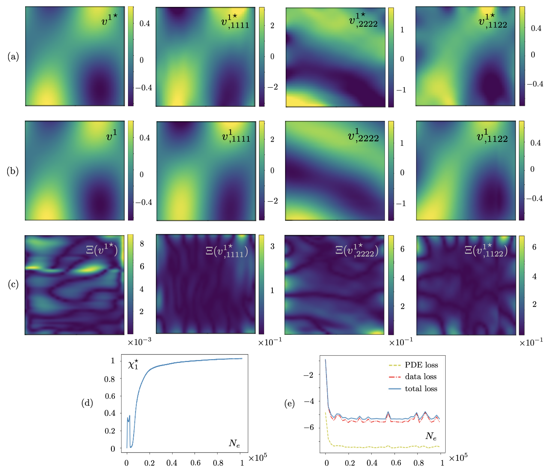
Following Section 3.3, PINNs are built and trained using experimental test data of Section 4.4. The MLP network with six hidden layers of respectively , , , , , and neurons is constructed to map the out-of-plane velocity field (in ) related to a single transducer location and frequency . The PDE parameter is defined as the unknown scaler parameter of the network, and following the argument of Section 3.3, the Lagrange multiplier is specified as a nonadaptive scaler weight of magnitude . The input/output dimension for is , and each epoch makes use of the full dataset for training and the learning rate is . Keep in mind that the objective here is to (a) construct a surrogate map for , and (b) identify .
Fig. 21 demonstrates (a) the accuracy of PINN-estimated field compared to the test data , (b) performance of automatic differentiation in capturing the fourth-order field derivatives e.g., that appear in the governing PDE (12), and (c) the evolution of parameter . The comparison in (b) is with respect to the spectral derivates of test data according to Section 2.3.2. It is no surprise that the automatic differentiation incurs greater errors in estimating the higher order derivatives involved in the antiplane wave motion compared to the second-order derivatives of Section 3.3.
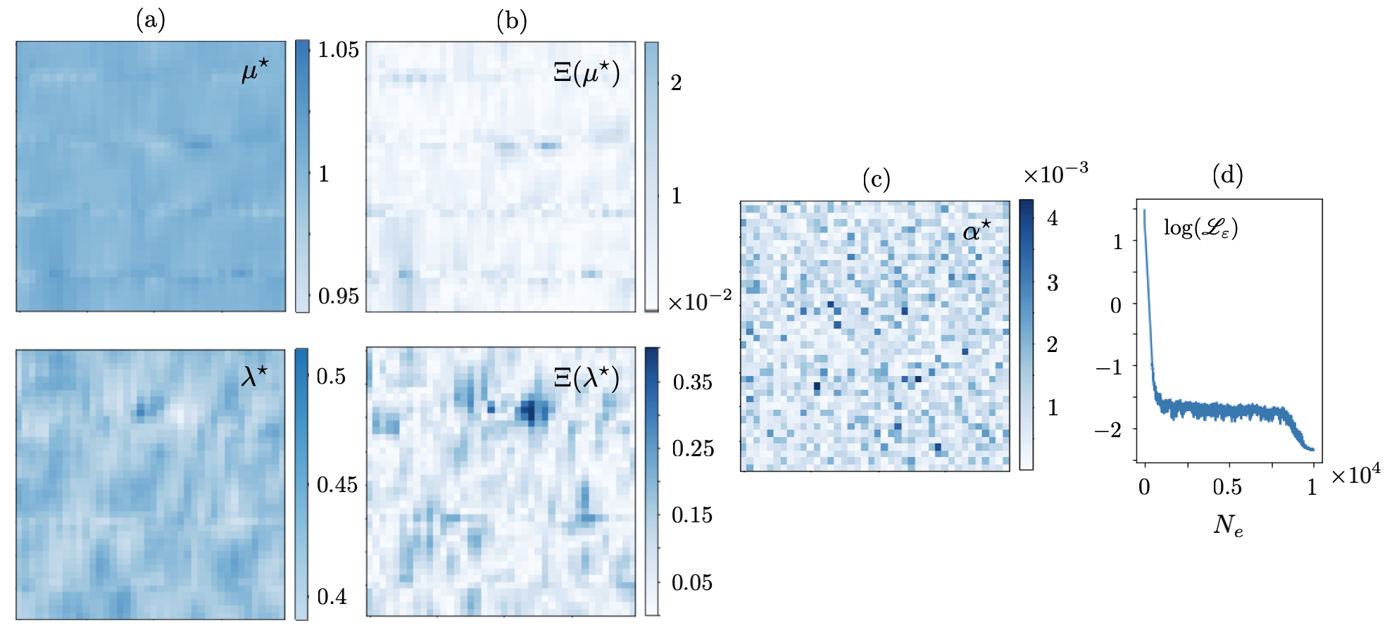
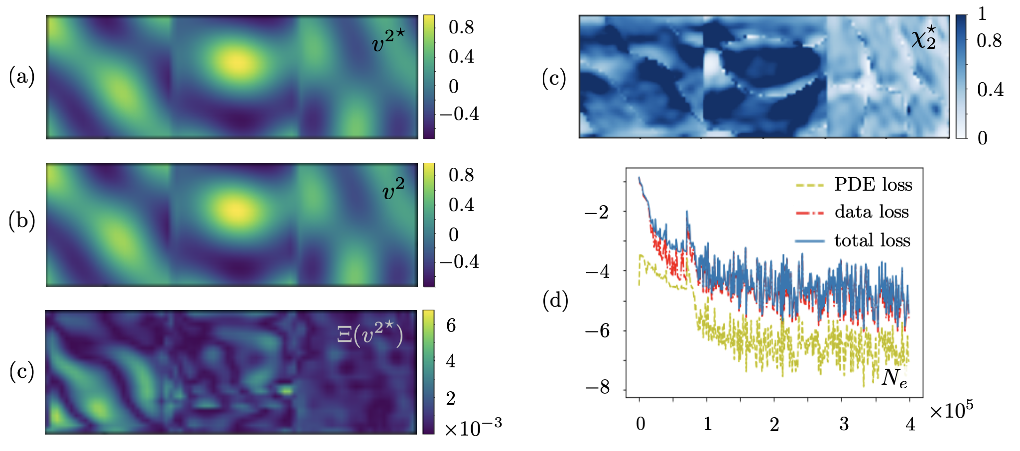
In addition, the PINN with seven hidden layers of respectively , , , , , , and neurons is created to reconstruct (i) particle velocity field in the layered specimen , and (ii) distribution of the PDE parameter in the sampling area. The latter is defined as an unknown parameter of the network with dimension , and the scaler weight is set to for the low-frequency reconstruction. In this setting, the input/output dimension for reads . Fig. 22 provides a comparative analysis between the experimental and PINN-predicted maps of velocity and PDE parameter. The associated statistics are provided in Table 9. It is evident from the waveform in Fig. 22 (a) that the most pronounced errors in Fig. 22 (d) occur at the loci of vanishing particle velocity. Similar to Section 3.2, this could be potentially addressed by enriching the test data.
5 Conclusions
The ML-based direct inversion and physics-informed neural networks are investigated for full-field ultrasonic characterization of layered components. Direct inversion makes use of signal processing tools to directly compute the field derivatives from dense datasets furnished by laser-based ultrasonic experiments. This allows for a simplified and controlled learning process that specifically recovers the sought-for physical fields through minimizing a single-objective loss function. PINNs are by design more versatile and particularly advantageous with limited test data where waveform completion is desired (or required) for mechanical characterization. PINNs multi-objective learning from ultrasonic data may be more complex but can be accomplished via carefully gauged loss functions.
In direct inversion, Tikhonov regularization is critical for stable reconstruction of distributed PDE parameters from limited or multi-fidelity experimental data. In this vein, deep learning offers a unique opportunity to simultaneously recover the regularization parameter as an auxiliary field which proved to be particularly insightful in inversion of experimental data.
In training PINNs, two strategies were remarkably helpful: (1) identifying the reference length scale by the dominant wavelength in an effort to control the norm of spatial derivatives – which turned out to be crucial in the case of flexural waves in thin plates with the higher order PDE, and (2) estimating the Lagrange multiplier by taking advantage of the inertia term in the governing PDEs.
Laboratory implementations at multiple frequencies exposed that verification and validation are indispensable for predictive data-driven modeling. More specifically, both direct inversion and PINNs recover the unknown “physical” quantities that best fit the data to specific equations (with often unspecified range of validity). This may lead to mathematically decent but physically incompatible reconstructions especially when the perceived physical laws are near their limits such that the discrepancy in capturing the actual physics is significant. In which case, the inversion algorithms try to compensate for this discrepancy by adjusting the PDE parameters which leads to non-physical reconstructions. Thus, it is paramount to conduct complementary experiments to (a) establish the applicability of prescribed PDEs, and (b) validate the predictive capabilities of the reconstructed models.
| | | | |
|---|---|---|---|
| | | |
Authors’ contributions
Y.X. investigation, methodology, data curation, software, visualization, writing – original draft; F.P. conceptualization, methodology, funding acquisition, supervision, writing – original draft; J.S. experimental data curation; C.W. experimental data curation.
Acknowledgments
This study was funded by the National Science Foundation (Grant No. 1944812) and the University of Colorado Boulder through FP’s startup. This work utilized resources from the University of Colorado Boulder Research Computing Group, which is supported by the National Science Foundation (awards ACI-1532235 and ACI-1532236), the University of Colorado Boulder, and Colorado State University. Special thanks are due to Kevish Napal for facilitating the use of FreeFem++ code developed as part of [49] for elastodynamic simulations.
References
- [1] X. Liang, M. Orescanin, K. S. Toohey, M. F. Insana, S. A. Boppart, Acoustomotive optical coherence elastography for measuring material mechanical properties, Optics letters 34 (19) (2009) 2894–2896.
- [2] G. Bal, C. Bellis, S. Imperiale, F. Monard, Reconstruction of constitutive parameters in isotropic linear elasticity from noisy full-field measurements, Inverse problems 30 (12) (2014) 125004.
- [3] B. S. Garra, Elastography: history, principles, and technique comparison, Abdominal imaging 40 (4) (2015) 680–697.
- [4] C. Bellis, H. Moulinec, A full-field image conversion method for the inverse conductivity problem with internal measurements, Proceedings of the Royal Society A: Mathematical, Physical and Engineering Sciences 472 (2187) (2016) 20150488.
- [5] H. Wei, T. Mukherjee, W. Zhang, J. Zuback, G. Knapp, A. De, T. DebRoy, Mechanistic models for additive manufacturing of metallic components, Progress in Materials Science 116 (2021) 100703.
- [6] C.-T. Chen, G. X. Gu, Learning hidden elasticity with deep neural networks, Proceedings of the National Academy of Sciences 118 (31) (2021) e2102721118.
- [7] H. You, Q. Zhang, C. J. Ross, C.-H. Lee, M.-C. Hsu, Y. Yu, A physics-guided neural operator learning approach to model biological tissues from digital image correlation measurements, arXiv preprint arXiv:2204.00205.
- [8] C. M. Bishop, N. M. Nasrabadi, Pattern recognition and machine learning, Vol. 4, Springer, 2006.
- [9] Y. LeCun, Y. Bengio, G. Hinton, Deep learning, nature 521 (7553) (2015) 436–444.
- [10] S. Cuomo, V. S. Di Cola, F. Giampaolo, G. Rozza, M. Raissi, F. Piccialli, Scientific machine learning through physics-informed neural networks: Where we are and what’s next, arXiv preprint arXiv:2201.05624.
- [11] S. Wang, H. Wang, P. Perdikaris, Improved architectures and training algorithms for deep operator networks, Journal of Scientific Computing 92 (2) (2022) 1–42.
- [12] L. McClenny, U. Braga-Neto, Self-adaptive physics-informed neural networks using a soft attention mechanism, arXiv preprint arXiv:2009.04544.
- [13] Z. Chen, V. Badrinarayanan, C.-Y. Lee, A. Rabinovich, Gradnorm: Gradient normalization for adaptive loss balancing in deep multitask networks, in: International conference on machine learning, PMLR, 2018, pp. 794–803.
- [14] M. Raissi, P. Perdikaris, G. E. Karniadakis, Physics informed deep learning (part i): Data-driven solutions of nonlinear partial differential equations, arXiv preprint arXiv:1711.10561.
- [15] M. Raissi, P. Perdikaris, G. E. Karniadakis, Physics-informed neural networks: A deep learning framework for solving forward and inverse problems involving nonlinear partial differential equations, Journal of Computational physics 378 (2019) 686–707.
- [16] E. Haghighat, M. Raissi, A. Moure, H. Gomez, R. Juanes, A physics-informed deep learning framework for inversion and surrogate modeling in solid mechanics, Computer Methods in Applied Mechanics and Engineering 379 (2021) 113741.
- [17] A. Henkes, H. Wessels, R. Mahnken, Physics informed neural networks for continuum micromechanics, Computer Methods in Applied Mechanics and Engineering 393 (2022) 114790.
- [18] R. Muthupillai, D. Lomas, P. Rossman, J. F. Greenleaf, A. Manduca, R. L. Ehman, Magnetic resonance elastography by direct visualization of propagating acoustic strain waves, science 269 (5232) (1995) 1854–1857.
- [19] P. E. Barbone, N. H. Gokhale, Elastic modulus imaging: on the uniqueness and nonuniqueness of the elastography inverse problem in two dimensions, Inverse problems 20 (1) (2004) 283.
- [20] O. A. Babaniyi, A. A. Oberai, P. E. Barbone, Direct error in constitutive equation formulation for plane stress inverse elasticity problem, Computer methods in applied mechanics and engineering 314 (2017) 3–18.
- [21] A. N. Tikhonov, A. Goncharsky, V. Stepanov, A. G. Yagola, Numerical methods for the solution of ill-posed problems, Vol. 328, Springer Science & Business Media, 1995.
- [22] A. Kirsch, et al., An introduction to the mathematical theory of inverse problems, Vol. 120, Springer, 2011.
- [23] On the convergence of physics informed neural networks for linear second-order elliptic and parabolic type pdes, Communications in Computational Physics 28 (5) (2020) 2042–2074.
- [24] S. Wang, X. Yu, P. Perdikaris, When and why pinns fail to train: A neural tangent kernel perspective, Journal of Computational Physics 449 (2022) 110768.
- [25] Z. Xiang, W. Peng, X. Liu, W. Yao, Self-adaptive loss balanced physics-informed neural networks, Neurocomputing 496 (2022) 11–34.
- [26] R. Bischof, M. Kraus, Multi-objective loss balancing for physics-informed deep learning, arXiv preprint arXiv:2110.09813.
- [27] H. Son, S. W. Cho, H. J. Hwang, Al-pinns: Augmented lagrangian relaxation method for physics-informed neural networks, arXiv preprint arXiv:2205.01059.
- [28] S. Zeng, Z. Zhang, Q. Zou, Adaptive deep neural networks methods for high-dimensional partial differential equations, Journal of Computational Physics 463 (2022) 111232.
- [29] J. Yu, L. Lu, X. Meng, G. E. Karniadakis, Gradient-enhanced physics-informed neural networks for forward and inverse pde problems, Computer Methods in Applied Mechanics and Engineering 393 (2022) 114823.
- [30] S. Wang, Y. Teng, P. Perdikaris, Understanding and mitigating gradient flow pathologies in physics-informed neural networks, SIAM Journal on Scientific Computing 43 (5) (2021) A3055–A3081.
- [31] A. D. Jagtap, K. Kawaguchi, G. Em Karniadakis, Locally adaptive activation functions with slope recovery for deep and physics-informed neural networks, Proceedings of the Royal Society A 476 (2239) (2020) 20200334.
- [32] Y. Kim, Y. Choi, D. Widemann, T. Zohdi, A fast and accurate physics-informed neural network reduced order model with shallow masked autoencoder, Journal of Computational Physics 451 (2022) 110841.
- [33] G. I. Barenblatt, Scaling (Cambridge texts in applied mathematics), Cambridge University Press, Cambridge, UK, 2003.
- [34] K. Hornik, Approximation capabilities of multilayer feedforward networks, Neural networks 4 (2) (1991) 251–257.
- [35] Y. Chen, L. Dal Negro, Physics-informed neural networks for imaging and parameter retrieval of photonic nanostructures from near-field data, APL Photonics 7 (1) (2022) 010802.
- [36] F. Pourahmadian, B. B. Guzina, On the elastic anatomy of heterogeneous fractures in rock, International Journal of Rock Mechanics and Mining Sciences 106 (2018) 259 – 268.
- [37] X. Liu, J. Song, F. Pourahmadian, H. Haddar, Time-vs. frequency-domain inverse elastic scattering: Theory and experiment, arXiv preprint arXiv:2209.07006.
- [38] F. Pourahmadian, B. B. Guzina, H. Haddar, Generalized linear sampling method for elastic-wave sensing of heterogeneous fractures, Inverse Problems 33 (5) (2017) 055007.
- [39] F. Cakoni, D. Colton, H. Haddar, Inverse Scattering Theory and Transmission Eigenvalues, SIAM, 2016.
- [40] V. A. Morozov, Methods for solving incorrectly posed problems, Springer Science & Business Media, 2012.
- [41] R. Kress, Linear integral equation, Springer, Berlin, 1999.
- [42] A. Paszke, S. Gross, S. Chintala, G. Chanan, E. Yang, Z. DeVito, Z. Lin, A. Desmaison, L. Antiga, A. Lerer, Automatic differentiation in pytorch.
- [43] H. Brezis, Functional analysis, Sobolev spaces and partial differential equations, Springer Science & Business Media, 2010.
- [44] T. Ha-Duong, On retarded potential boundary integral equations and their discretization, in: Topics in computational wave propagation, Springer, 2003, pp. 301–336.
- [45] R. T. Rockafellar, Lagrange multipliers and optimality, SIAM review 35 (2) (1993) 183–238.
- [46] H. Everett III, Generalized lagrange multiplier method for solving problems of optimum allocation of resources, Operations research 11 (3) (1963) 399–417.
- [47] D. Liu, Y. Wang, A dual-dimer method for training physics-constrained neural networks with minimax architecture, Neural Networks 136 (2021) 112–125.
-
[48]
F. Hecht, New development in freefem++, Journal of
Numerical Mathematics 20 (3-4) (2012) 251–265.
URL https://freefem.org/ - [49] F. Pourahmadian, K. Napal, Poroelastic near-field inverse scattering, Journal of Computational Physics 455 (2022) 111005.
- [50] A. Paszke, S. Gross, F. Massa, A. Lerer, J. Bradbury, G. Chanan, T. Killeen, Z. Lin, N. Gimelshein, L. Antiga, A. Desmaison, A. Kopf, E. Yang, Z. DeVito, M. Raison, A. Tejani, S. Chilamkurthy, B. Steiner, L. Fang, J. Bai, S. Chintala, Pytorch: An imperative style, high-performance deep learning library, Advances in neural information processing systems 32.
- [51] D. P. Kingma, J. Ba, Adam: A method for stochastic optimization, arXiv preprint arXiv:1412.6980.
- [52] Pytorch implementation of physics-informed neural networks, https://github.com/jayroxis/PINNs (2022).
- [53] K. F. Graff, Wave motion in elastic solids, Courier Corporation, 2012.