Deep Learning COVID-19 Features on CXR using Limited Training Data Sets
Abstract
Under the global pandemic of COVID-19, the use of artificial intelligence to analyze chest X-ray (CXR) image for COVID-19 diagnosis and patient triage is becoming important. Unfortunately, due to the emergent nature of the COVID-19 pandemic, a systematic collection of CXR data set for deep neural network training is difficult. To address this problem, here we propose a patch-based convolutional neural network approach with a relatively small number of trainable parameters for COVID-19 diagnosis. The proposed method is inspired by our statistical analysis of the potential imaging biomarkers of the CXR radiographs. Experimental results show that our method achieves state-of-the-art performance and provides clinically interpretable saliency maps, which are useful for COVID-19 diagnosis and patient triage.
Index Terms:
COVID-19, Chest X-Ray, Deep Learning, Segmentation, Classification, Saliency MapI Introduction
Coronavirus disease 2019 (COVID-19), caused by severe acute respiratory syndrome coronavirus 2 (SARS-CoV-2), has become global pandemic in less than four months since it was first reported, reaching a 3.3 million confirmed cases and 238,000 death as of May 2nd, 2020. Due to its highly contagious nature and lack of appropriate treatment and vaccines, early detection of COVID-19 becomes increasingly important to prevent further spreading and to flatten the curve for proper allocation of limited medical resources.
Currently, reverse transcription polymerase chain reaction (RT-PCR), which detects viral nucleic acid, is the golden standard for COVID-19 diagnosis, but RT-PCR results using nasopharyngeal and throat swabs can be affected by sampling errors and low viral load [1]. Antigen tests may be fast, but have poor sensitivity.
Since most COVID-19 infected patients were diagnosed with pneumonia, radiological examinations may be useful for diagnosis and assessment of disease progress. Chest computed tomography (CT) screening on initial patient presentation showed outperforming sensitivity to RT-PCR [2] and even confirmed COVID-19 infection on negative or weakly-positive RT-PCR cases [1]. Accordingly, recent COVID-19 radiological literature primarily focused on CT findings [3, 2]. However, as the prevalence of COVID-19 increases, the routine use of CT places a huge burden on radiology departments and potential infection of the CT suites; so the need to recognize COVID-19 features on chest X-ray (CXR) is increasing.
Common chest X-ray findings reflect those described by CT such as bilateral, peripheral consolidation and/or ground glass opacities [3, 2]. Specifically, Wong et al [4] described frequent chest X-ray (CXR) appearances on COVID-19. Unfortunately, it is reported that chest X-ray findings have a lower sensitivity than initial RT-PCR testing (69% versus 91%, respectively) [4]. Despite this low sensitivity, CXR abnormalities were detectable in 9% of patients whose initial RT-PCR was negative.
As the COVID-19 pandemic threatens to overwhelm healthcare systems worldwide, CXR may be considered as a tool for identifying COVID-19 if the diagnostic performance with CXR is improved. Even if CXR cannot completely replace the RT-PCR, the indication of pneumonia is a clinical manifestation of patient at higher risk requiring hospitalization, so CXR can be used for patient triage, determining the priority of patients’ treatments to help saturated healthcare system in the pandemic situation. This is especially important, since the most frequent known etiology of community acquired pneumonia is bacterial infection in general [5]. By excluding these population by triage, limited medical resource can be spared substantially.

Accordingly, deep learning (DL) approaches on chest X-ray for COVID-19 classification have been actively explored [6, 7, 8, 9, 10, 11, 12]. Especially, Wang et al [6] proposed an open source deep convolutional neural network platform called COVID-Net that is tailored for the detection of COVID-19 cases from chest radiography images. They claimed that COVID-Net can achieve good sensitivity for COVID-19 cases with 80% sensitivity.
Inspired by this early success, in this paper we aim to further investigate deep convolutional neural network and evaluate its feasibility for COVID-19 diagnosis. Unfortunately, under the current public health emergency, it is difficult to collect large set of well-curated data for training neural networks. Therefore, one of the main focuses of this paper is to develop a neural network architecture that is suitable for training with limited training data set, which can still produce radiologically interpretable results. Since most frequently observed distribution patterns of COVID-19 in CXR are bilateral involvement, peripheral distribution and ground-glass opacification (GGO) [13], a properly designed neural network should reflect such radiological findings.
To achieve this goal, we first investigate several imaging biomarkers that are often used in CXR analysis, such as lung area intensity distribution, the cardio-thoracic ratio, etc. Our analysis found that there are statistically significant differences in the patch-wise intensity distribution, which is well-correlated with the radiological findings of the localized intensity variations in COVID-19 CXR. This findings lead us to propose a novel patch-based deep neural network architecture with random patch cropping, from which the final classification result are obtained by majority voting from inference results at multiple patch locations. One of the important advantages of the proposed method is that due to the patch training the network complexity is relative small and multiple patches in each image can be used to augment training data set, so that even with the limited data set the neural network can be trained efficiently without overfitting. By combining with our novel preprocessing step to normalize the data heterogeneities and bias, we demonstrate that the proposed network architecture provides better sensitivity and interpretability, compared to the existing COVID-Net [6] with the same data set.
Furthermore, by extending the idea of the gradient-weighted class activation map (Grad-CAM) [14], yet another important contribution of this paper is a novel probabilistic Grad-CAM that takes into account of patch-wise disease probability in generating global saliency map. The resulting class activation map clearly show the interpretable results that are well correlated with radiological findings.
II Proposed Network Architecture
The overall algorithmic framework is given in Fig. 1. The CXR images are first pre-processed for data normalization, after which the pre-processed data are fed into a segmentation network, from which lung areas can be extracted as shown in Fig. 1(a). From the segmented lung area, classification network is used to classify the corresponding diseases using a patch-by-patch training and inference, after which the final decision is made based on the majority voting as shown in Fig. 1(b). Additionally, a probabilistic Grad-CAM saliency map is calculated to provide an interpretable result. In the following, each network is described in detail.
II-A Segmentation network
Our segmentation network aims to extract lung and heart contour from the chest radiography images. We adopted an extended fully convolutional (FC)-DenseNet103 to perform semantic segmentation [15]. The training objective is
| (1) |
where is the cross entropy loss of multi-categorical semantic segmentation and denotes the network parameter set, which is composed of filter kernel weights and biases. Specifically, is defined as
| (2) |
where is the indicator function, denotes the softmax probability of the -th pixel in a CXR image , and denotes the corresponding ground truth label. denotes class category, i.e., {background, heart, left lung, right lung}. denotes weights given to each class category.
CXR images from different dataset resources may induce heterogeneity in their bits depth, compression type, image size, acquisition condition, scanning protocol, postprocessing, etc. Therefore, we develop a universal preprocessing step for data normalization to ensure uniform intensity histogram throughout the entire dataset. The detailed preprocessing steps are as follows:
-
1.
Data type casting (from uint8/uint16 to float32)
-
2.
Histogram equalization (gray level = [0, 255.0])
-
3.
Gamma correction ( = 0.5)
-
4.
Image resize (height, width = [256, 256])
Using the preprocessed data, we trained FC-DenseNet103[15] as our backbone segmentation network architecture. Network parameters were initialized by random distribution. We applied Adam optimizer [16] with an initial learning rate of 0.0001. Whenever training loss did not improve by certain criterion, the learning rate was reduced by factor 10. We adopted early stopping strategy based on validation performance. Batch size was optimized to 2. We implemented the network using PyTorch library [17].
II-B Classification network
The classification network aims to classify the chest X-ray images according to the types of disease. We adopted the relatively simple ResNet-18 as the backbone of our classification algorithm for two reasons. The first is to prevent from overfitting, since it is known that overfitting can occur when using an overly complex model for small number of data. Secondly, we intended to do transfer learning with pre-trained weights from ImageNet to compensate for the small training data set. We found that these strategy make the training stable even when the dataset size is small.
The labels were divided into four classes: normal, bacterial pneumonia, tuberculosis (TB), and viral pneumonia which includes the pneumonia caused by COVID-19 infection. We assigned the same class for viral pneumonia from other viruses (e.g. SARS-cov or MERS-cov) with COVID-19, since it is reported that they have similar radiologic features even challenging for the experienced radiologists [18]. Rather, we concentrated on more feasible work such as distinguishing bacterial pneumonia or tuberculosis from viral pneumonia, which show considerable differences in the radiologic features and are still useful for patient triage.
The pre-processed images were first masked with the lung masks from the segmentation networks, which are then fed into a classification network. Classification network were implemented in two different versions: global and local approaches. In the global approach, the masked images were resized to , which were fed into the network. This approach is focusing on the global appearance of the CXR data, and was used as a baseline network for comparison. In fact, many of the existing researches employs similar procedure [6, 7, 8, 9].
In the local patch-based approach, which is our proposed method, the masked images were cropped randomly with a size of , and resulting patches were used as the network inputs as shown in Fig. 1(b). In contrast to the global approach, various CXR images are resized to a much bigger image for our classification network to reflect the original pixel distribution better. Therefore, the segmentation mask from Fig. 1(a) are upsampled to match the image size. To avoid cropping the patch from the empty area of the masked image, the centers of patches were randomly selected within the lung areas. During the inference, -number of patches were randomly acquired for each image to represent the entire attribute of the whole image. The number was chosen to sufficiently cover all lung pixels multiple times. Then, each patch was fed into the network to generate network output, and among network output the final decision was made based on majority voting, i.e. the most frequently declared class were regarded as final output as depicted in Fig. 1(b). In this experiments, the number of random patches was set to 100, which means that 100 patches were generated randomly from one whole image for majority voting.
For network training, pre-trained parameters from ImageNet are used for network weight initialization, after which the network was trained using the CXR data. As for optimization algorithm, Adam optimizer [16] with learning rate of 0.00001 was applied. The network were trained for 100 epochs, but we adopted early stopping strategy based on validation performance metrics. The batch size of 16 was used. We applied weight decay and regularization to prevent overfitting problem. The classification network was also implemented by Pytorch library.
II-C Probabilistic Grad-CAM saliency map visualization
We investigate the interpretability of our approach by visualizing a saliency map. One of the most widely used saliency map visualization methods is so-called gradient weighted class activation map (Grad-CAM) [14]. Specifically, the Grad-CAM saliency map of the class for a given input image is defined by
| (3) |
where is the -th feature channel at the last convolution layer (which corresponds to the layer 4 of ResNet-18 in our case), denotes the upsampling operator from a feature map to the image, is the rectified linear unit (ReLU) [14]. Here, is the feature weighted parameter for the class , which can be obtained by
| (4) |
for some scaling parameter , where is the score for the class before the softmax layer and denotes the -th pixel value of . The Grad-CAM map is then normalized to have value in . The Grad-CAM for the global approach is used as a baseline saliency map.
However, care should be taken in applying Grad-CAM to our local patch-based approach, since each patch has different score for the COVID-19 class. Therefore, to obtain the global saliency map, patch-wise Grad-CAM saliency maps should be weighted with the estimated probability of the class, and their average value should be computed. More specifically, our probabilistic Grad-CAM with respect to the input image has the following value at the -th pixel location:
| (5) |
where denotes the -th input patch, refers to the operator that copies the -size -th patch into the appropriate location of a zero-padded image in , and denotes the Grad-CAM computed by (3) with respect to the input patch , and denotes the number of the frequency of the -th pixel in the total patches. Additionally, the class probability for the -th patch can be readily calculated after the soft-max layer. Accordingly, the average probability of each pixel belonging to a given class can be taken into consideration in Eq. (5) when constructing a global saliency map.
III Method
III-A Dataset
We used public CXR datasets, whose characteristics are summarized in Table I and Table II. In particular, the data in Table I are used for training and validation of the segmentation networks, since the ground-truth segmentation masks are available. The curated data in Table II are from some of the data in Table I as well as other COVID-19 resources, which were used for training, validation, and test for the classification network. More detailed descriptions of the dataset are follows.
III-A1 Segmentation network dataset
The JSRT dataset was released by the Japanese Society of Radiological Technology (JSRT) [19]. Total 247 chest posteroanterior (PA) radiographs were collected from 14 institutions including normal and lung nodule cases. Corresponding segmentation masks were collected from the SCR database [20]. The JSRT/SCR dataset were randomly split into training (80%) and validation (20%). For cross-database validation purpose, we used another public CXR dataset: U.S. National Library of Medicine (USNLM) collected Montgomery Country (MC) dataset [21]. Total 138 chest PA radiographs were collected including normal, tuberculosis cases and corresponding lung segmentation masks.
| Dataset | Class | # | Bits | Mask | |
| Lung | Heart | ||||
| Training | |||||
| JSRT/SCR[19][20] | Normal/Nodule | 197 | 12 | O | O |
| Validation | |||||
| JSRT/SCR | Normal/Nodule | 50 | 12 | O | O |
| NLM(MC)[21] | Normal | 73 | 8 | O | - |
| Dataset | Class | # | Bits | Mask | |
|---|---|---|---|---|---|
| Lung | Heart | ||||
| JSRT/SCR | Normal | 20 | 12 | O | O |
| NLM(MC) | Normal | 73 | 8 | O | - |
| CoronaHack[22] | Normal | 98 | 24 | - | - |
| NLM(MC) | Tuberculosis | 57 | 8 | O | - |
| CoronaHack | Pneumonia (Bacteria) | 21 | 24 | - | - |
| Cohen et al[23] | Pneumonia (Bacteria) | 33 | 24 | - | - |
| Pneumonia (Virus) | 20 | 24 | - | - | |
| Pneumonia (COVID-19) | 180 | 24 | - | - | |
III-A2 Classification dataset
The dataset resources for the classification network are described in Table II. Specifically, for normal cases, the JSRT dataset and the NLM dataset from the segmentation validation dataset were included. For comparing COVID-19 from normal and different lung diseases, data were also collected from different sources [23, 22], including additional normal cases. These datasets were selected because they are fully accessible to any research group, and they provide the labels with detailed diagnosis of disease. This enables more specific classification of pneumonia into bacterial and viral pneumonia, which should be classified separately because of their distinct clinical and radiologic differences.
In the collected data from the public dataset[22], over 80% was pediatric CXR from Guangzhou Women and Children’s Medical Center [24]. Therefore, to avoid the network from learning biased features from age-related characteristics, we excluded pediatric CXR images. This is because we aim to utilize CXR radiography with unbiased age distribution for more accurate evaluation of deep neural networks for COVID-19 classification.
| Dataset | Normal | Bacterial | Tuberculosis | Viral | COVID-19 | Total |
|---|---|---|---|---|---|---|
| Training | 134 | 39 | 41 | 14 | 126 | 354 |
| Validation | 19 | 5 | 5 | 2 | 18 | 49 |
| Test | 38 | 10 | 11 | 4 | 36 | 99 |
| Total | 191 | 54 | 57 | 20 | 180 | 502 |
Total dataset was curated into five classes; normal, tuberculosis, bacterial pneumoia, viral pneumonia, COVID-19 pneumonia. The numbers of each disease class from the data set are summarized in Table III. Specifically, a total of 180 radiography images of 118 subjects from COVID-19 image data collection were included. Moreover, a total of 322 chest radiography images from different subjects were used, which include 191, 54, and 20 images for normal, bacterial pneumonia, and viral pneumonia (not including COVID-19), respectively. The combined dataset were randomly split into train, validation, and test sets with the ratio of 0.7, 0.1, and 0.2.
III-A3 Dataset for comparison with COVID-Net
We prepared a separate dataset to compare our method with existing state-of-the art (SOTA) algorithm called COVID-Net [6]. COVID-19 image data collection was combined with RSNA Pneumonia Detection Challenge dataset as described in [6] for a fair comparison between our method and COVID-Net. The reason we separately train our network with the COVID-Net data set is that RSNA Pneumonia Detection Challenge dataset provide only the information regarding the presence of pneumonia, rather than the detailed diagnosis of disease, so that the labels were divided into only three categories including normal, pneumonia, and COVID-19 as in Table IV. More specifically, there were 8,851 normal and 6,012 pneumonia chest radiography images from 13,645 patients in RSNA Pneumonia Detection Challenge dataset, and these images were combined with COVID-19 image data collection to compose a total dataset. Among these, 100 normal, 100 pneumonia, and 10 COVID-19 images were randomly selected for validation and test set, respecitvely as in [6]. Although we believe our categorization into normal, bacterial, TB, and viral+COVID-19 cases is more correlated with the radiological findings and practically useful in clinical environment [18], we conducted this additional comparison experiments with the data set in Table IV to demonstrate that our algorithm provides competitive performance compared to COVID-Net in the same experiment set-up.
| Dataset | Normal | Pneumonia | COVID-19 | Total |
|---|---|---|---|---|
| Training | 8651 | 5812 | 160 | 14623 |
| Validation | 100 | 100 | 10 | 210 |
| Test | 100 | 100 | 10 | 210 |
| Total | 8851 | 6012 | 180 | 15043 |
III-B Statistical Analysis of Potential CXR COVID-19 markers
The following standard biomarkers from CXR image analysis are investigated.
-
•
Lung morphology: Morphological structures of the segmented lung area as illustrated in Fig. 2(b) was evaluated throughout different classes.
-
•
Mean lung intensity: From the segmented lung area, we calculated mean value of the pixel intensity within the lung area as shown in Fig. 2(c).
-
•
Standard deviation of lung intensity: From the intensity histogram of lung area pixels, we calculated one standard deviation which is indicated as the black double-headed arrow in Fig. 2(c).
-
•
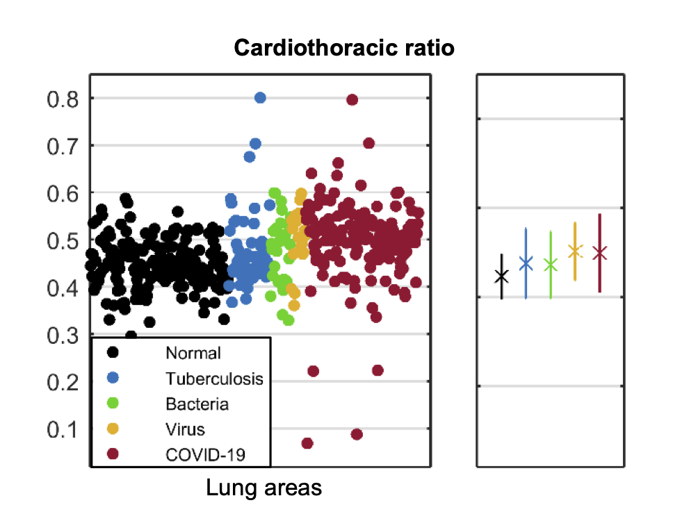
Cardiothoracic Ratio (CTR): CTR can be calculated by dividing the maximal transverse cardiac diameter by the maximal internal thoracic diameter annotated repectively as red and blue double-headed arrows in Fig. 2(a). Cardiothoracic Ratio (CTR) is a widely used marker to diagnosis cardiomegaly [25, 26]. We hypothesized that if cardiothoracic boundary become blurred by rounded opacities or consolidation in COVID-19 CXR [3, 2, 4], distinct off-average CTR value can be utilized as an abnormality alarm.
Statistical analysis for the potential biomarkers was performed using MATLAB 2015a (Mathworks, Natick). Kolmogorov Smirnov test was used to evaluate the normal distribution of marker candidates. For non-normally distributed variables, Wilcoxon signed rank test was used to compare segmentation performance with identical data size, and Wilcoxon rank sum test was used to compare COVID-19 marker candidates to those of other classes with different data sizes. Statistical significance (SS) levels were indicated as asterisks; * for 0.05, ** for 0.01 and *** for 0.001.

III-C Classification performance metrics
The performance of the classification methods was evaluated using the confusion matrix. From the confusion matrix, true positive (TP), true negative (TN), false positive (FP), and false negative (FN) values were obtained, and 5 metrics for performance evaluation were calculated as below:
-
1.
-
2.
-
3.
-
4.
-
5.
Among these, the F1 score was used as the evaluation metric for early stopping. The overall metric scores of the algorithm were calculated by averaging each metric for multiple classes.
IV EXPERIMENTAL RESULTS
IV-A Segmentation performance on cross-database
Segmentation performance of anatomical structure was evaluated using Jaccard similarity coefficient. Table V presents the Jaccard similarity coefficient of each contour on the validation dataset. The results confirmed our method provides comparable accuracy to previous works using the JSRT dataset and the NLM(MC) dataset [27, 28].
| Preprocess | Jaccard similarity coefficient | |||
|---|---|---|---|---|
| Lung | SS | Heart | ||
| JSRT | O | 0.9550.015 | 0.8890.054 | |
| NLM(MC) | - | 0.9320.022 | *** | |
| NLM(MC) | O | 0.9430.013 | ||
To evaluate segmentation performance on cross-database, we tested either original or preprocessed images of the NLM dataset as inputs. The result shows that our universal preprocessing step for data normalization contributes to the processing of cross-database with statistically significant improvement on segmentation accuracy (Jaccard similarity coefficients from 0.932 to 0.943, 0.001). This result indicates that preprocessing is crucial factor to ensure segmentation performance in cross-database.
IV-B Morphological analysis of lung area
To analyze morphological characteristics in the segmented lung area, a representative CXR radiograph for each class was selected for visual evaluation. Lung contour of each class showed differentiable features and showed mild tendency. In normal and tuberculosis cases (the first and the second row of Fig. 3, respectively), overall lung and heart contour were well-segmented. In the bacterial case, however, the segmented lung area was deformed due to wide spread opacity of bacterial pneumonia as shown in the third row of Fig. 3, and both the right cardiac and thoracic borders were lost. In overall bacterial infection cases, similar findings were occasionally observed which caused degraded segmentation performance. This suggests that abnormal morphology of the segmentation masks may be a useful biomarker to differentiate the severe infections. In the fourth row of Fig. 3, viral infection caused bilateral consolidations [29], thus partial deformation of lung area was observed. In the COVID-19 case of the fifth row of Fig. 3, despite the bi-basal infiltrations [30], lung area was fully segmented. In overall cases of the viral and the COVID-19 classes, lung areas were either normally or partially-imcompletely segmented, so morphological features of the segmentation masks may not be sufficiently discriminatory markers for viral and COVID-19 classes. Based on these morphological findings in segmented lung area, we further investigated other potential COVID-19 biomarkers.


IV-C Statistical significancy of potential COVID-19 bio-markers
We hypothesized that CXR appearance influenced by consolidations or infiltration of COVID-19 may be reflected in intensity of the radiograph. Thus, intensity-related COVID-19 marker candidates were extracted and compared.
IV-C1 Lung areas intensity
Mean pixel intensity of each lung area is shown in the scatter plot of Fig. 4(a). COVID-19 cases showed lower mean intensity compared to other cases with statistical significance level (0.001 for normal and bacterial, 0.01 for TB). Table VI describes the corresponding statistical result. Despite the statistical significance, the scatter plot showed broad overlap between several classes.
| Mean | STD | Statistical significance | ||||
|---|---|---|---|---|---|---|
| Normal | TB | Bacteria | Viral | |||
| Normal | 0.540 | 0.055 | ||||
| Tuberculosis | 0.523 | 0.043 | * | |||
| Bacteria | 0.558 | 0.054 | - | *** | ||
| Viral | 0.509 | 0.047 | ** | - | *** | |
| COVID-19 | 0.506 | 0.051 | *** | ** | *** | - |
IV-C2 Lung areas intensity variance
Standard deviation of pixel intensity of each lung area are scattered in plot in Fig. 4(b). For both the COVID-19 and the viral cases, the variance values were higher than other classes with statistical significance (0.001 for all). Table VII describes the corresponding statistical result.
| Mean | STD | Statistical significance | ||||
|---|---|---|---|---|---|---|
| Normal | TB | Bacteria | Viral | |||
| Normal | 0.139 | 0.017 | ||||
| Tuberculosis | 0.136 | 0.016 | - | |||
| Bacteria | 0.145 | 0.019 | * | ** | ||
| Viral | 0.165 | 0.022 | *** | *** | *** | |
| COVID-19 | 0.163 | 0.022 | *** | *** | *** | - |
| Mean | STD | Statistical significance | ||||
|---|---|---|---|---|---|---|
| Normal | TB | Bacteria | Viral | |||
| Normal | 0.139 | 0.017 | ||||
| Tuberculosis | 0.136 | 0.016 | - | |||
| Bacteria | 0.143 | 0.020 | - | - | ||
| Viral | 0.163 | 0.025 | *** | *** | ** | |
| COVID-19 | 0.161 | 0.022 | *** | *** | *** | - |
To investigate the effect of scanning protocol on statistics, we performed additional study by excluding AP Supine radiographs from entire dataset with documented patient information. Recall that AP Supine protocol is an alternative to standard PA or AP protocol depending on patient condition. Since AP Supine protocol is not common in normal cases, supine scanning with different acquisition condition may have potential for considerable heterogeneity in data distribution, causing biased results in statistical analysis, so we investigated this issue. The result shown in Table VIII compared to Table VII showed minor difference in both the COVID-19 and the viral and cases. The result indicates that for both the COVID-19 and viral classes, the highly intensity-variable characteristic in the lung area is invariant to scaning protocol.
IV-C3 Cardiothoracic ratio
CTR values of each lung area is scattered in Fig. 4(c). Despite there exist statistical differences between the COVID-19 cases to other classes (0.001 for normal and TB, 0.05 for Bacteria), the scatter plot showed broad overlap between several classes. Table IX describes the corresponding statistical result.
| Mean | STD | Statistical significance | ||||
|---|---|---|---|---|---|---|
| Normal | TB | Bacteria | Viral | |||
| Normal | 0.446 | 0.051 | ||||
| Tuberculosis | 0.476 | 0.078 | * | |||
| Bacteria | 0.472 | 0.074 | - | - | ||
| Viral | 0.502 | 0.064 | *** | * | - | |
| COVID-19 | 0.499 | 0.086 | *** | *** | * | - |
Based on the statistical analysis of potential bio-marker candidates, we found that intensity distribution pattern within the lung area may be most effective in the diagnosis, which highly reflects the reported chest X-ray (CXR) appearances of COVID-19, i.e., multi-focally distributed consolidation and GGO in specific region such as peripheral and lower zone [3, 2, 4].
However, care should be taken, since not only the locally concentrated multiple opacities can cause uneven intensity distribution throughout entire lung area, but also different texture distribution within CXR may cause the similar intensity variations. For example, multi-focally distributed consolidation from COVID-19 could make the intensity variance differentiating factor from other classes, but also bacterial pneumonia generates opacity as well, whose feature may lead to the similar intensity distributions as results of different characteristics of opacity spreading pattern.
To decouple these compounding effects, we further investigated the local and global intensity distribution. For the correctly classified patches from our classification network, we computed their mean intensity and standard deviation (STD) values. We refer to the distribution of mean intensity of each patch as the inter-patch intensity distribution (Fig. 5(a)) and the STD of each patch as intra-patch intensity distribution (Fig. 5(b)). As shown in Fig. 5(a), the inter-patch intensity distribution of the unified COVID-19 and viral class showed distict lower intensity values (0.001 for all) to other classes and highly intensity-variant characteristics which can be represented as the large error bar. This result is in accordance with the result of lung area intensity and intensity variance (Fig. 4(a), (b)). Intra-patch intensity distribution, however, showed no difference compared to the normal class (0.05). From these intra- and inter-patch intensity distribution results, we can infer that intra-patch variance, which represents local texture information, was not crucially informative, whereas the globally distributed multi-focal intensity change may be an important discriminating feature for COVID-19 diagnosis, which is strongly correlated with the radiological findings.


One common finding among the marker candidates was no difference between the COVID-19 and the viral case (0.05 for all the markers), which is also correlated with radiological findings [18]. Therefore, in the classification network, the COVID-19 and viral classes were integrated into one class.
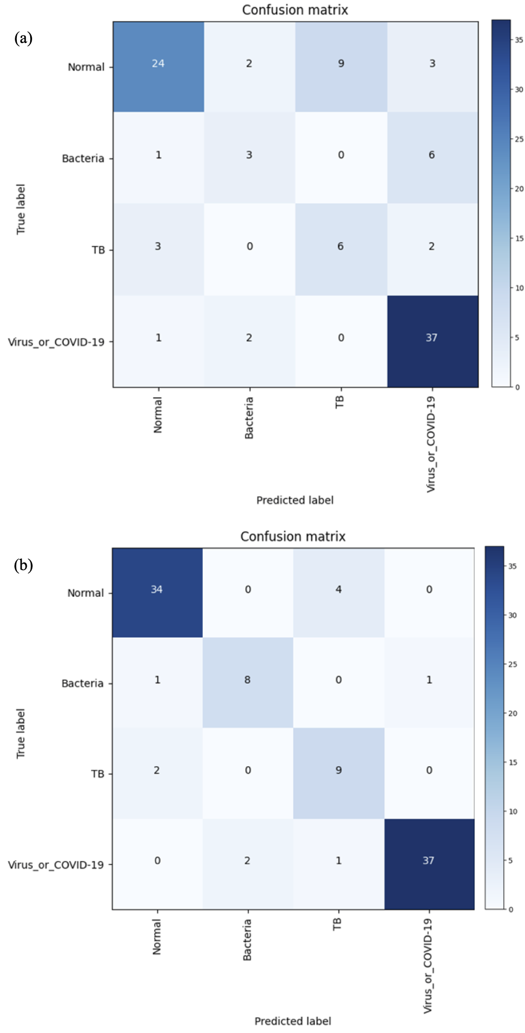
IV-D Classification performance
The classification performances of the proposed method are provided in Table X. The confusion matrices for the (a) global method and the (b) local patch-based method are shown in Fig. 6. The proposed local patch-based approach showed consistently better performance than global approach in all metrics. In particular, as depicted in Table XI, our method showed the sensitivity of for COVID-19 and viruses, which was acceptable performance as a screening method, considering the fact that the sensitivity of COVID-19 diagnosis by X-ray image is known to be even for clinical experts and that the current gold standard, RT-PCR, has sensitivity of [4]. Moreover, compared to the global approach, the sensitivity of other classes are significantly high, which confirms the efficacy of our method.
| Methods | Accuracy | Precision | Recall | F1 score | Specificity |
|---|---|---|---|---|---|
| Global approach | 70.7 | 60.6 | 60.1 | 59.3 | 89.7 |
| Local approach | 88.9 | 83.4 | 85.9 | 84.4 | 96.4 |
| Methods | Sensitivity | |||
|---|---|---|---|---|
| Normal | bacterial | Tuberculosis | COVID-19 and Viral | |
| Global approach | 63.2 | 30 | 54.5 | 92.5 |
| Local approach | 89.5 | 80 | 81.8 | 92.5 |


IV-E Interpretability using saliency map
Fig. 7 and Fig. 8 illustrate the examples of visualization of saliency map. As shown in Fig. 7(a), the existing Grad-CAM method for global approach showed the limitation that it only focuses on the broad main lesion so that it cannot properly differentiate multifocal lesions within the image. On the other hand, with the probabilistic Grad-CAM, multifocal GGOs and consolidations were visualized effectively by our local patch-based approach as shown in Fig. 7(c), which was in consistent with the findings reported by clinical experts. In particular, when we compute the probabilistic Grad-CAM for the COVID-19 class using patient images from various classes (i.e., normal, bacterial, TB, and COVID-19), a noticeable activation map was observed only in the COVID-19 patient data set, whereas almost no activations were observed in patients with other diseases and conditions as shown in Fig. 8. These results strongly support our claim that the probabilistic Grad-CAM saliency map from our local patch-based approach is more intuitive and interpretable compared to the existing methods.
V Discussion
V-A COVID-19 Features on CXR
In the diagnosis of COVID-19, other diseases mimicking COVID-19 pneumonia should be differentiated, including community-acquired pneumonia such as streptococcus pneumonia, mycoplasma and chlamydia related pneumonia, and other coronavirus infections.
In radiological literature, most frequently observed distribution patterns of COVID-19 are bilateral involvement, peripheral distribution and ground-glass opacification (GGO) [13]. Wong et al [4] found that consolidation was the most common finding (30/64, 47%), followed by GGO (21/64, 33%). CXR abnormalities had a peripheral (26/64, 41%) and lower zone distribution (32/64, 50%) with bilateral involvement (32/64, 50%), whereas pleural effusion was uncommon (2/64, 3%).
Our statistical analysis of the intensity distribution clearly showed that the globally distributed localized intensity variation is a discriminatory factor for COVID-19 CXR images, which was also confirmed with our saliency map. This clearly confirmed that the proposed method clearly reflects the radiological findings.
V-B Feasibility as a ‘triage’ for COVID-19
In pandemic situation of infectious disease, the distribution of medical resources is a matter of the greatest importance. As COVID-19 is spreading rapidly and surpassing the capacity of medical system in many countries, it is necessary to make reasonable decision to distribute the limited resources based on the ‘triage’, which determine the needs and urgency for each patient. In general, the most common cause of community acquired pneumonia is bacterial infection [5]. Specifically, most studies reported that S. pneumoniae is the most frequent causative strain (), after which H. influenza () and viral pneumonia follow as the second and the third most common causes of pneumonia, respectively [5]. In addition, depending on the geological region, substantial proportion of pneumonia may be diagnosed as tuberculosis (up to ) [5]. Summing these up, the proportion of bacterial pneumonia and tuberculosis is suspected to be still large even in this pandemic situation of COVID-19. In this respect, the disease such as bacterial pneumonia or tuberculosis as well as normal condition can be excluded primarily, to preserve limited medical resources such as RT-PCR or CT only for those who suspected to be infected with COVID-19.
The detailed triage workflow that utilizes the proposed algorithm is described in Fig. 9. Specifically, our neural network is trained to classify other viral and COVID-19 in the same class. This is not only because it is strongly correlated with the radiological findings [18], but also useful as a triage. More specifically, by excluding normal, bacterial pneumonia, and TB at the early stage, we can use RT-PCR or CT for only those patients classified as other virus and COVID-19 cases for final diagnosis. By doing this procedure, we can save limited medical resources such as RT-PCR or CT to those patients whose diagnosis by CXR is difficult even by radiologists.

V-C Training stability
In order to investigate the origin of the apparent advantages of using local patch-based training over the global approach, we investigate the training dynamics to investigate the presence of overfitting. This is especially important, given that the training data is limited due to the difficulty of systematic CXR data collection for COVID-19 cases under current public health emergency.
Fig. 10 shows the curves for accuracy and F1 score of (a) the global approach and (b) the proposed local patch-based approach for each epoch. Note that both approaches use the same number of weight parameters. Still, thanks to the increasing training data set from the random patch cropping across all image area, our local patch-based algorithm did not showed any sign of overfitting even with the small numbers of training data, while the global approach showed significant overfitting problem. This clearly indicates that with the limited data set the patch-based neural network training may be a promising direction.

V-D Comparison with COVID-Net
Since the proposed patch-based neural network architecture is designed by considering limited training data set, we investigated any potential performance loss in comparison with other state-of-the art (SOTA) deep learning approach that has been developed without such consideration. Specifically, COVID-Net [6] is one of the most successful approaches in COVID-19 diagnosis, so we chose it as the SOTA method.
The comparison between our method and COVID-Net is shown in Table XII. With the same dataset, our method showed overall accuracy of 91.9 % which is comparable to that of 92.4 % for COVID-Net. Furthermore, our method provided significantly improved sensitivity to COVID-19 cases compared to the COVID-Net. In addition, it is also remarkable that our method uses only about 10% number of parameters (11.6 M) compared to that of COVID-Net (116.6 M), because the proposed algorithm is developed based on less complex network architecture without increasing the complexity of the model. This may bring the advantages not only in the aspect of computational time but also in the aspect of performance and stability with small-sized dataset.
| Methods | Sensitivity | Precision | ||||
|---|---|---|---|---|---|---|
| Normal | Pneumonia | COVID-19 | Normal | Pneumonia | COVID-19 | |
| COVID-Net | 95 | 91 | 80 | 91.3 | 93.8 | 88.9 |
| Proposed | 90 | 93 | 100 | 95.7 | 90.3 | 76.9 |
V-E Cross-database generalization capability
We are aware that the current study has limitations due to the lack of well-curated pneumonia CXR dataset. Specifically, our CXR data set come from a single or at most two sources (see Table II). Moreover, publicly available COVID-19 dataset [23] are largely extracted from online publications, website, etc, so they are not collected in a rigorous manner.
To mitigate the issue of potential bias from the limitation of the database, we employed a universal preprocessing step for data normalization for the entire dataset as discussed before. We investigated the effects of our preprocessing step on cross-database generalization by investigating the COVID-19 dataset, which poses the most severe intra-dataset heterogeneity. As shown in Fig. 11(b), each original CXRs of the COVID-19 class showed highly-varying intensity characteristics among each segmented anatomies. Thanks to our preprocessing step, the mean pixel intensity distribution between lung and heart regions of the preprocessed COVID-19 dataset (see Fig. 11(c)) became similar to the normal class in Fig. 11(a). The problem of heterogeneity can be also mitigated as shown in the intensity histograms (see Fig. 11(d)-(f)). The results confirmed that the original COVID-19 data could be well preprocessed to have comparable intensity distribution to that of well-curated normal data.

V-F Segmentation network analysis
V-F1 Comparison with U-Net
Recall that we chose FC-DenseNet103 as a backbone segmentation network architecture thanks to its higher segmentation performance with smaller number of parameters (9.4 M)[31]. To demonstrate the effectiveness of CXR segmentation by the FC-Densenet103, we trained U-Net [32] under identical training conditions and compared the results. There was no significant difference between the networks result.
| Networks | Lung jaccard similarity coefficient | |||
|---|---|---|---|---|
| JSRT | SS | NLM(MC) | SS | |
| U-Net | 0.9550.014 | 0.05 | 0.9410.014 | 0.05 |
| FC-DenseNet103 | 0.9550.015 | 0.9430.013 | ||
We further analyzed the effect of the different segmentation methods on classification performance. The proposed segmentation method with the FC-DenseNet103 resulted consistently better classification performance in all metrics than the U-Net. When compared with the FC-DenseNet67, which has smaller number of parameters (3.5 M) [15], the performance improvement by our method is significant. Given the better trade-off between the complexity versus performance, we adopted FC-DenseNet103 as our segmentation network.
| Netowrks | Accuracy | Precision | Recall | F1 score | Specificity |
|---|---|---|---|---|---|
| U-Net | 85.9 | 82.3 | 84 | 82.5 | 95.3 |
| FC-DenseNet67 | 81.8 | 73.1 | 76.6 | 74.3 | 91.5 |
| FC-DenseNet103 | 88.9 | 83.4 | 85.9 | 84.4 | 96.4 |
V-F2 Effect of trainset size
To demonstrate the robustness of the proposed segmentation network with limited training dataset, we performed the ablation study by reducing training dataset size. Lung segmentation performance was evaluated on the cross-database NLM(MC) dataset. For the preprocessed NLM(MC) dataset, Jaccard similarity coefficients remain stable until 50% of trainset was used for training as shown in Table XV; however, in the original NLM(MC) dataset without preprocessing step, segmentation performance decreased steeply as the size of trainsets decreased. This results support that proposed segmentation network endures limited training dataset size by matching intensity distribution of cross-database CXRs thanks to our preprocessing step.
| Trainset size | Lung jaccard similarity coefficient | |||
|---|---|---|---|---|
| NLM | SS | NLM(MC) | SS | |
| (preprocessed) | 100% | (original) | 100% | |
| 100% | 0.9430.013 | 0.9320.022 | ||
| 50% | 0.9410.018 | 0.05 | 0.9080.035 | *** |
| 30% | 0.9290.025 | *** | 0.8660.047 | *** |
| 10% | 0.9060.045 | *** | 0.8510.058 | *** |
V-F3 Segmentation effects on marker analysis and classification
The proposed segmentation network was trained with normal subject set that have segmentation mask as shown Table V, XV, and showed comparable performance with the state-of-the-art for the normal subjects. However, when CXR images with severe consolidation are used, segmentation performance degradation is unavoidable, since such images have been never observed during the training.
For example, the radiograph from a bacterial pneumonia case in Fig. 3 was under-segmented due to widely spread severe opacity. To further investigate this issue, we examined all cases of under-segmentation by defining the under-segmentation as a segmentation mask in which over 1/4 of the entire lung region is deformed. Our investigation showed that the under-segmentations are only outliers that are observed in some patient data set (7 of 54 bacterials cases (13%,), 2 of 57 cases for TB (3.5%), and 5 of 200 cases for COVID-19 and viral pneumonia (2.5%)), whereas no under segmentation were observed from 191 healthy subjects.
To confirm that the difference in the segmentation results can be a morphological marker for classification, we evaluated whether it is possible to distinguish normal and abnormal images (including bacterial pneumonia, tuberculosis, COVID-19 and other viruses) using only binary segmentation masks (not X-ray images). With a separately trained neural network using only binary masks, it was possible to distinguish between normal and abnormal images with 86.9% sensitivity. This confirms that the morphology of the segmentation mask is a discriminatory biomarker between normal and the patient groups. Then, we conducted additional experiments to evaluate how classification performance is affected by excluding or including under-segmentation cases. Although the differences in other labels were not significant, the overall sensitivity for bacterial were better when the under-segmented subjects were excluded. Therefore, the under-segmentation still has some effects on the classification between the diseases.
Finally, we performed an additional experiment for the comparison of classification with and without segmentation masks. The results in Table XVI clearly confirmed that despite the under-segmented outliers the use of segmentation mask significantly improved the classification performance on the whole. This suggests that there are rooms to improve the performance of the proposed method, if the segmentation network could be further trained using patient cases with correct segmentation labels.
| Methods | Accuracy | Precision | Recall | F1 score | Specificity |
|---|---|---|---|---|---|
| Without mask | 79.8 | 72.7 | 59.7 | 60.7 | 91.9 |
| With mask | 88.9 | 83.4 | 85.9 | 84.4 | 96.4 |
V-G Classification network analysis
V-G1 Effect of patch size on the performance
To evaluate the effect of the patch size on the performance of the classification algorithm, we tested various patch sizes, such as , and . Using half-sized () patches, the results were worse as shown in Table XVII. With double-sized () patches, the results were not better than those with patch size of , as depicted in Table XVII. In summary, there seems to be a clear drawback in reducing the patch size, and there was also no benefit with increasing the patch size. Therefore, we chose the value in between.
| Patch size | Accuracy | Precision | Recall | F1 score | Specificity |
|---|---|---|---|---|---|
| 78.8 | 71.2 | 75.9 | 72.3 | 93.2 | |
| 88.9 | 83.4 | 85.9 | 84.4 | 96.4 | |
| 84.8 | 78.8 | 80.1 | 79.3 | 94.8 |
V-G2 Effects of trainset size
We analyzed the effect of dataset size in terms of classification performance, since we aimed to develop the method that has the advantage of maintaining robustness even when only limited data are available. The classification performances with decreasing dataset sizes are provided in Fig. 12. The global approach using whole image, which is similar to most classification methods, showed prominent decrease in accuracy with decreasing dataset size, but the proposed local patch-based method showed less compromised performance, showing the robustness to the reduced dataset size as shown in Fig. 12(a). These results were more prominent when comparing them by relative scale as shown in Fig. 12(b).

VI Conclusion
In the rapidly evolving global pandemic of COVID-19, the use of CXR for COVID-19 diagnosis or triage for patient management has become an important issue to preserve limited medical resources and prevent further spreading of the virus. However, the current diagnostic performance with CXR is not sufficient for routine clinical use, so the need of artificial intelligence to improve diagnostic performance of CXR is increasing. Unfortunately, due to the emergent nature of COVID-19 global pandemic, systematic collection of the large data set for deep neural network training is difficult.
To address this problem, we investigated potential biomarkers in the CXR and found the globally distributed localized intensity variation can be an discrimatory feature for the COVID-19. Based on this finding, we propose a patch-based deep neural network architecture that can be stably trained with small data set. Once the neural network was trained, the final decision was made based on the majority voting from multiple patches at random locations within lungs. We also proposed a novel probabilistic Grad-CAM saliency map that is tailored to the local patch-based approach. Our experimental results demonstrated that the proposed network was trained stably with small data set, provided comparative results with the SOTA method, and generated interpretable saliency maps that are strongly correlated with the radiological findings.
Acknowledgment
We would like to thank the doctors and medical professionals from Korea and all around the world who have dedicated their time and efforts to treat COVID-19 patients and protect the health of citizens during this pandemic. This work was supported by the National Research Foundation of Korea under Grant NRF-2020R1A2B5B03001980.
References
- [1] X. Xie, Z. Zhong, W. Zhao, C. Zheng, F. Wang, and J. Liu, “Chest CT for typical 2019-ncov pneumonia: relationship to negative RT-PCR testing,” Radiology, p. 200343, 2020.
- [2] Y. Fang, H. Zhang, J. Xie, M. Lin, L. Ying, P. Pang, and W. Ji, “Sensitivity of chest CT for COVID-19: comparison to RT-PCR,” Radiology, p. 200432, 2020.
- [3] T. Ai, Z. Yang, H. Hou, C. Zhan, C. Chen, W. Lv, Q. Tao, Z. Sun, and L. Xia, “Correlation of chest CT and RT-PCR testing in coronavirus disease 2019 (COVID-19) in China: a report of 1014 cases,” Radiology, p. 200642, 2020.
- [4] H. Y. F. Wong, H. Y. S. Lam, A. H.-T. Fong, S. T. Leung, T. W.-Y. Chin, C. S. Y. Lo, M. M.-S. Lui, J. C. Y. Lee, K. W.-H. Chiu, T. Chung et al., “Frequency and distribution of chest radiographic findings in COVID-19 positive patients,” Radiology, p. 201160, 2020.
- [5] P. D. Brown and S. A. Lerner, “Community-acquired pneumonia,” The Lancet, vol. 352, no. 9136, pp. 1295–1302, 1998.
- [6] L. Wang and A. Wong, “COVID-net: A tailored deep convolutional neural network design for detection of COVID-19 cases from chest radiography images,” arXiv preprint arXiv:2003.09871, 2020.
- [7] A. Narin, C. Kaya, and Z. Pamuk, “Automatic detection of coronavirus disease (COVID-19) using X-ray images and deep convolutional neural networks,” arXiv preprint arXiv:2003.10849, 2020.
- [8] I. D. Apostolopoulos and T. A. Mpesiana, “COVID-19: automatic detection from x-ray images utilizing transfer learning with convolutional neural networks,” Physical and Engineering Sciences in Medicine, p. 1, 2020.
- [9] E. E.-D. Hemdan, M. A. Shouman, and M. E. Karar, “COVIDX-Net: A framework of deep learning classifiers to diagnose COVID-19 in X-ray images,” arXiv preprint arXiv:2003.11055, 2020.
- [10] I. Apostolopoulos, S. Aznaouridis, and M. Tzani, “Extracting possibly representative COVID-19 biomarkers from X-ray images with deep learning approach and image data related to pulmonary diseases,” arXiv preprint arXiv:2004.00338, 2020.
- [11] M. Farooq and A. Hafeez, “COVID-ResNet: a deep learning framework for screening of COVID19 from radiographs,” arXiv preprint arXiv:2003.14395, 2020.
- [12] P. Afshar, S. Heidarian, F. Naderkhani, A. Oikonomou, K. N. Plataniotis, and A. Mohammadi, “COVID-CAPS: A capsule network-based framework for identification of COVID-19 cases from X-ray Images,” arXiv preprint arXiv:2004.02696, 2020.
- [13] S. Salehi, A. Abedi, S. Balakrishnan, and A. Gholamrezanezhad, “Coronavirus disease 2019 (COVID-19): a systematic review of imaging findings in 919 patients,” American Journal of Roentgenology, pp. 1–7, 2020.
- [14] R. R. Selvaraju, M. Cogswell, A. Das, R. Vedantam, D. Parikh, and D. Batra, “Grad-cam: Visual explanations from deep networks via gradient-based localization,” in Proceedings of the IEEE international conference on computer vision, 2017, pp. 618–626.
- [15] S. Jégou, M. Drozdzal, D. Vazquez, A. Romero, and Y. Bengio, “The one hundred layers tiramisu: Fully convolutional densenets for semantic segmentation,” in Proceedings of the IEEE conference on computer vision and pattern recognition workshops, 2017, pp. 11–19.
- [16] D. P. Kingma and J. Ba, “Adam: A method for stochastic optimization,” arXiv preprint arXiv:1412.6980, 2014.
- [17] A. Paszke, S. Gross, S. Chintala, G. Chanan, E. Yang, Z. DeVito, Z. Lin, A. Desmaison, L. Antiga, and A. Lerer, “Automatic differentiation in PyTorch,” in NIPS Autodiff Workshop, 2017.
- [18] S. H. Yoon, K. H. Lee, J. Y. Kim, Y. K. Lee, H. Ko, K. H. Kim, C. M. Park, and Y.-H. Kim, “Chest radiographic and CT findings of the 2019 novel coronavirus disease (COVID-19): analysis of nine patients treated in Korea,” Korean Journal of Radiology, vol. 21, no. 4, pp. 494–500, 2020.
- [19] J. Shiraishi, S. Katsuragawa, J. Ikezoe, T. Matsumoto, T. Kobayashi, K.-i. Komatsu, M. Matsui, H. Fujita, Y. Kodera, and K. Doi, “Development of a digital image database for chest radiographs with and without a lung nodule,” American Journal of Roentgenology, vol. 174, no. 1, pp. 71–74, Jan 2000. [Online]. Available: https://doi.org/10.2214/ajr.174.1.1740071
- [20] B. Van Ginneken, M. B. Stegmann, and M. Loog, “Segmentation of anatomical structures in chest radiographs using supervised methods: a comparative study on a public database,” Medical image analysis, vol. 10, no. 1, pp. 19–40, 2006.
- [21] S. Jaeger, S. Candemir, S. Antani, Y.-X. J. Wáng, P.-X. Lu, and G. Thoma, “Two public chest X-ray datasets for computer-aided screening of pulmonary diseases,” Quantitative imaging in medicine and surgery, vol. 4, no. 6, p. 475, 2014.
- [22] Praveen. CoronaHack: Chest X-Ray-Dataset. (2020, Mar 21). [Online]. Available: https://www.kaggle.com/praveengovi/coronahack-chest-xraydataset
- [23] J. P. Cohen, P. Morrison, and L. Dao, “COVID-19 image data collection,” arXiv 2003.11597, 2020. [Online]. Available: https://github.com/ieee8023/covid-chestxray-dataset
- [24] D. S. Kermany, M. Goldbaum, W. Cai, C. C. Valentim, H. Liang, S. L. Baxter, A. McKeown, G. Yang, X. Wu, F. Yan et al., “Identifying medical diagnoses and treatable diseases by image-based deep learning,” Cell, vol. 172, no. 5, pp. 1122–1131, 2018.
- [25] C. S. Danzer, “The cardiothoracic ratio: an index of cardiac enlargement.” The American Journal of the Medical Sciences (1827-1924), vol. 157, no. 4, p. 513, 1919.
- [26] K. Dimopoulos, G. Giannakoulas, I. Bendayan, E. Liodakis, R. Petraco, G.-P. Diller, M. F. Piepoli, L. Swan, M. Mullen, N. Best et al., “Cardiothoracic ratio from postero-anterior chest radiographs: a simple, reproducible and independent marker of disease severity and outcome in adults with congenital heart disease,” International journal of cardiology, vol. 166, no. 2, pp. 453–457, 2013.
- [27] S. Candemir and S. Antani, “A review on lung boundary detection in chest X-rays,” International journal of computer assisted radiology and surgery, vol. 14, no. 4, pp. 563–576, 2019.
- [28] E. Jangam and A. Rao, “Public datasets and techniques for segmentation of anatomical structures from chest x-rays: Comparitive study, current trends and future directions,” in International Conference on Recent Trends in Image Processing and Pattern Recognition. Springer, 2018, pp. 321–331.
- [29] N. S. Paul, H. Roberts, J. Butany, T. Chung, W. Gold, S. Mehta, E. Konen, A. Rao, Y. Provost, H. H. Hong et al., “Radiologic pattern of disease in patients with severe acute respiratory syndrome: the toronto experience,” Radiographics, vol. 24, no. 2, pp. 553–563, 2004.
- [30] I. Thevarajan, T. H. Nguyen, M. Koutsakos, J. Druce, L. Caly, C. E. van de Sandt, X. Jia, S. Nicholson, M. Catton, B. Cowie et al., “Breadth of concomitant immune responses prior to patient recovery: a case report of non-severe COVID-19,” Nature Medicine, pp. 1–3, 2020.
- [31] D. Lobo Torres, R. Queiroz Feitosa, P. Nigri Happ, L. Elena Cué La Rosa, J. Marcato Junior, J. Martins, P. Olã Bressan, W. N. Gonçalves, and V. Liesenberg, “Applying fully convolutional architectures for semantic segmentation of a single tree species in urban environment on high resolution uav optical imagery,” Sensors, vol. 20, no. 2, p. 563, 2020.
- [32] O. Ronneberger, P. Fischer, and T. Brox, “U-net: Convolutional networks for biomedical image segmentation,” in International Conference on Medical image computing and computer-assisted intervention. Springer, 2015, pp. 234–241.